http://www.sciencepublishinggroup.com/j/ijdsa doi: 10.11648/j.ijdsa.20190506.11
ISSN: 2575-1883 (Print); ISSN: 2575-1891 (Online)
Bayesian Spatial-temporal Modelling and Mapping for
Crime Data in Nairobi County
George Ngogoyo Chege
*, Samuel Musili Mwalili, Anthony Wanjoya
Department of Statistics and Actuarial Science, Jomo Kenyatta University of Agriculture and Technology (Jkuat), Nairobi, Kenya
Email address:
*
Corresponding author
To cite this article:
George Ngogoyo Chege, Samuel Musili Mwalili, Anthony Wanjoya. Bayesian Spatial-temporal Modelling and Mapping for Crime Data in Nairobi County. International Journal of Data Science and Analysis. Vol. 5, No. 6, 2019, pp. 111-116. doi: 10.11648/j.ijdsa.20190506.11
Received: October 8, 2019; Accepted: October 29, 2019; Published: November 4, 2019
Abstract:
Nairobi is a county in Kenya that is more prone to crime occurrence. This has made many researchers, for the past years, to study about crime occurrence in its suburbs and which factors promote crime. The theories around crime are always coupled with an attempt to predict their occurrence, for better crime analysis, and management, in case they happen, the associated covariates and their changes are analyzed. At the sub-county level, the crime occurrence is highly studied and understood. In this study, using Bayesian theory, this study builds spatial-temporal Bayesian model approach to crime to analyze its spatial-temporal patterns and determine any developing trends using data regarding robberies that occurred in Nairobi County in Kenya from January 1, 2011 to December 31, 2018. Of the diverse socio-economic variables associated with crime rate, including unemployment rate, poverty, weak law enforcement, Alcohol and drug abuse, and illiteracy, this study finds that robbery crime rate is significantly correlated with the poverty index and the unemployment rate. This finding provides a statistical reference for County safety protection. For further work, we recommend that further study can be done to determine factors associated with the dynamics and the distribution of crime in Nairobi County while accounting for measurement error that might be present in thecovariates.Keywords:
Crime, Integrated Nested Laplace Approximation (INLA), Bayesian, Spatial-temporal Modeling, Hotspot, Crime Mapping1. Introduction
With the quickening urbanization in Kenya, urban crime has progressively turned out to be one of the real difficulties confronting Kenyan urban communities which have turned out to be increasingly various and separated along social and conservative classes. The fast modernization and urbanization has heightened the danger of criminal exploitation City government, approach producers, and policing organizations all perceive the significance of better understanding the elements of urban crime so as to control the crime. The main problem is that the government expenditure on security has increased from 7.5% of the GDP in 2014/15 to 7.97% in 2017/2018 to cater for security personnel and resource allocation to curb crime.
Crime being designed, choices to perpetrate violations are Designed, and the way toward carrying out Crimes are
additionally designed [1]. In this manner, breaking down Crime designs and foreseeing Crime patterns is essential to decreasing the rate of crime. With this marvel, it is feasible for the police to know when assets are best designated to an individual area and for to what extent, and when assets ought to be distributed to a neighborhood [2]. The far reaching utilization of geographic Information Systems (GIS) with the advancement of R-INLA method and programming for example, Win BUGS, Bayesian methodologies are being connected to the examination of numerous social and wellbeing issues, In particular, the utilization of Bayesian measurements for breaking down crime data was considered by these studies [3, 4].
examples of urban crime can give vital data about violations and structure fundamental bases in the advancement of hypothetical clarifications and powerful policing practices. As pointed out when inspecting China’s crime designs amid a time of quick social change will make an imperative commitment to the writing, and give vital experiences into the advancement of hypothetical clarifications [5].
Nevertheless, these studies include only spatial parameters and do not recognize temporal variability. Using Bayesian spatial-temporal models, it is convenient to process observations from more than one location and time period, integrating spatial, temporal, and spatial-temporal interaction information. Therefore, Bayesian spatial-temporal modelling approaches-specifically approaches that employ spatial and temporal random effects to analyze local patterns over time are popularly used in spatial epidemiological studies. Spatial-temporal using Bayesian approach is mainly used to study the mapping of disease distribution over a small region, geographic clusters of disease, and the correlation of diseases [6].
The existing research conducted by using Bayesian Spatial-temporal considering local variations in crime changes in space and time scale while predicting future crimes. To investigate the Influence of on premise and off-premise alcohol outlets on reported violent crime in the region of Waterloo, Ontario, application of the Bayesian spatial modeling to inform land use planning and policy [7].
A spatial-temporal analysis of community policing in Nairobi’s suburbs was done by considering Communities as neighborhood guardians, they first identified spatial hotspots using the space-time scan statistic based on the difference between observed and expected counts within ellipses centered at small-area centroids, and extends the spatial ellipse over time to analyze the persistence of spatial hotpots, While useful for identifying overall levels of space-time clustering for a dataset, testing-based methods do not identify overall spatial and temporal patterns and do not provide risk estimates for observations not identified as hotspots [8].
For this study, we considered crime that happened in Kenya, Nairobi County from January 1, 2011 to December 31, 2018. A spatial-temporal Bayesian approach is utilized to examine the spatial-temporal circulation designs dependent on chronicled information, to investigate the connections among crime and socio-economic factors (e.g., poverty index, unemployment rate, and illiteracy) and to show the patterns in crime. The bits of knowledge acquired gives critical references to crime expectation and its management.
2. Methodology
2.1. Study Area and Data Source
Nairobi County is Located in Kenya, East Africa, and it is divided into seventeen administrative units called sub-counties. These sub-counties are of different sizes and also vary in the Population of people who stay there. The data was obtained from annual Statistical abstract and reports from
KNBS, Kenya Police annual report and the World Bank Reports.
2.2. Study Variables
The dependent variable is the robbery crime rate which was defined as the crimes reported per 1000 inhabitants. Independent Variables are poverty rate, unemployment rate, illiteracy rate, Weak law enforcement and Alcohol, drug and substance abuse.
2.3. Statistical Analysis Methods
2.3.1. Introduction
A Bayesian approach was implemented to develop a model aimed both at the description of relative risk for robbery crime in space and time in Nairobi county. During the last three decades, Bayesian methods have been suffering significant advances and are starting to be extensively recognized in many investigation areas [9].
2.3.2. Bayesian Statistics
Bayesian statistics have a huge influence from conditional probability and more so in the theorem of Bayes which is defined as:
| = | ∗ (1)
The theorem follows the ideas developed by Bayes and Laplace regarding inverse probability: the probability of an event B, given that an event A occurs. So, it all occurs following the process: is computed before the event A is observed; then the is computed and used to access the and | is then accessed. In this sense, is the information on the event of interest available a priori, without carrying any experiment this probability will affect the posterior probability of . Thus, the will be dictated both by the prior information, as well as by the results of the experiment itself [9].
2.3.3. Bayesian Inference
We assume a realizations of a random variable
=
, …
whose density belongs to the parametric family = : ; ∈ Ψ . However, in the Bayesian approach, parameters of a distribution are treated as random variables for which we can specify prior distributions. The specification of prior distributions enables one to supplement the information provided by the data. It can also be argued that since different analysts specify different priors, this may lead to subjective inferences. Suppose we model observations,= , …
using the probability density function : .The likelihood function for is given as;
| = ! " !|#$ # (3)
Because is not a function of θ, the Bayes theorem can be re-written as;
| ∝ ∗ | (4) i.e. posterior
∝
prior * likelihoodWith the difficulty in computing in equation (3) we will use of simulation techniques INLA method in software R as an alternative to MCMC to approximate the posterior marginal because it has significantly reduces the computation time.
2.4. R-INLA: The Integrated Nested Laplace Approximation
The Algorithm INLA algorithm was introduced by H. Rue. It is a deterministic algorithm for Bayesian inference. This is the key-point that makes it different from MCMC, because these are based in simulations. INLA is specially developed for LGM’s and provides accurate results for an improved computing time, when compared to MCMC [10].
LGM’s or structure additive regression models, are a widely used class of models in statistical applications they include, amongst others, generalized linear models, smoothing, spline models, spatial and spatial-temporal models, log Gaussian Cox-processes and geostatistical and geo-additive models. The very first step to define a latent Gaussian model within the Bayesian framework is to identify a distribution for the observed data
= , …
. As a general approach, it is specified a distribution for characterized by a parameter &. This parameter is given by a function of a structured additive predictor hi through a link function . , such that . = ( in this sense, the additive linear predictor ( is given by:( = )*+ ∑. )-
- - + ∑"/ 0/ (5)
The terms . , can assume different forms such as smooth and nonlinear effects of covariates, time trends, temporal or spatial random effects. For this reason, the latent Gaussian models can be used in a wide range of applications, from generalized and dynamic linear models, to spatial and spatial-temporal models. In this sense, all latent (non-observable) components of interest are collected, in a set of parameters designated by = )*, ), is needed to specify a vector 1 of hype- parameters such as
= , …
2By assuming conditional independence, the distribution of 3 observations is given by a likelihood:4| , = ∏ 4 | , (6) Where each data point 4 is connected to one element in the latent field . On the logarithm, it is assumed a multivariate normal prior on , with mean 0, and precision matrix 5 , i.e., ~7 0, 59 , with density function given by:
| = 2 ;<=|5 = >exp B
C 5 5D (7)
This specification is known as Gaussian Markov random field, where the components of the latent Gaussian field are supposed to be conditionally independent with the consequence that 5 , is a sparse precision matrix.
2.5. Review of the Spatial-temporal Bayesian Models
2.5.1. Besag Model
In order to capture spatial dependence, we make use of a conditional autoregressive (CAR) model referred to as the Besag Model [11]. CAR Model is used to model spatial random variables and it is specified by a set of n univariate full conditional distribution.
Let
& = & , … &
denote a random variable which follows a CAR model under the specification it follows that.& |&E, F ≠ H, I ∼ 7 B K∑ &∼E E L KD (8)
where 3 is the number of neighbors of node i, i ~ j indicates that the two nodes i and j are neighbors, d > 0 is an extra term added on the diagonal controlling the "properness" I > 0 is a "precision-like" (or scaling) parameter that control the strength of the spatial association
.
2.5.2. BYM Model
The Besag-York-Mollie (BYM) Model specification [12]. The benefit is that this model allows to get the posterior marginal of the sum of the spatial and i.i.d model only assumes a spatially structured component and cannot take the limiting form that allows for no spatially structured variability. Hence, unstructured random error or pure over dispersion within an area will be modelled as spatial correlation, using an intrinsic conditional autoregressive structure (iCAR).
Under this specification it is assumed that the spatial random effect is drawn from a normal distribution whose mean is the mean of the neighbors random effects, with variance proportional to one over the number of neighbors (so more neighbors, less variability). The borrowing strength. Under the ICAR specification, we have;
N |NE∼ 7 B-K∑ NEO E,PQ=KD (9)
Where 3 is the number of sub counties adjacent to sub county i.
N,E= R1, F H T3U F TVW 3WFXYZ[V\0, Z]ℎWV_F\W
the specification of the ICAR model, the conditional distribution of given the remaining components (NE) is
normal with mean N and variance PQ=
K.
2.5.3. Random Walk of Order 1: RW1
Random walk which is a random process consisting of a sequence of discrete steps of fixed length. A distribution is said to follow a random walk if the first differences (difference between two successive observations) are random. In a random walk model, the series itself is not random, however, its differences are. The differences are independent, identically distributed random variables with a common distribution. The implication of using this model is that the crime count in one year in a sub-county depends largely on the results of the previous year. It is defined as
bc= bc9 + d (10)
2.6. Spatial-temporal Analysis
The model assumes that, conditional on the underlying relative risk ec, the number of counts in each area and time period c, follows a Poisson distribution, namely,
c~ ZF\\Z3 ec (11) f c = ec= W gc c (12) The log-risk is modeled taking into account the need of distinguishing between space and time components, and including interaction in space and time. More precisely, we assumed that;
log c = k + )# + N + l + mc+ c+ `c (13) Where mc and c represents the structured and unstructured temporal effect terms respectively, N T3U l captures the unstructured and structured spatial effects and `c represents the spatial-temporal interaction term, which expresses the Variation of time trends across the sub-counties.
2.7. Model Validation
The model was fitted in R using the R-INLA which has default set priors has and results were exported and mapped in QGIS. Assessment was done using the DIC [13].
The DIC is a generalization of the Akaike information criterion for evaluating Bayesian hierarchical modelling and has been the most widely used statistic for comparing the fitness of Bayesian spatial-Temporal models. It balances model goodness fit and complexity. It is defined as;
nop = nq + gr (14) Where nq is the posterior mean of the deviance of the model and gris the effective number of parameters. Smaller values of the DIC indicate a better trade-off between complexity and fit of the model.
3. Results and Discussion
3.1. Exploratory Data Analysis
The data used was yearly robbery crime data from the period January 1, 2011 to December 31, 2018, which constituted poverty rate, unemployment rate, illiteracy rate, Weak law enforcement and Alcohol, drug and substance abuse.
3.2. Estimation of the Model Parameters
To analyze hotspots and determine crime trends, we evaluated the spatial-temporal Bayesian model of robbery crime count assuming Poisson distribution. We then used the INLA simulation to sample the posterior distributions of the parameters. We set the number of annealing iterations to 50,000 after conducting 100,000 iterations, and use the residual samples for statistical inference. To reduce the dependency among samples, the dilution ratio was set to 50:1. Finally, we obtained the main parameter estimation results of the model according to the posterior distribution samples, as listed in Table 2.
The following seven equations were fitted using equation (11)
Model 1: log c = k + )# + N + l Model 2: log c = k + )# + mc+ c
Model 3: log c = k + )# + N + l + mc+ c Model 4: log c = k + )# + N + l + mc+ c+ `c In particular, the convolution model (TYPE I).
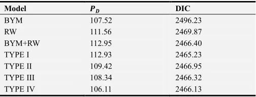
Provides the smallest DIC value. Thus, it is the best model in terms of goodness-of-fit measures. Model 4 is a spatial-temporal model with four different interactions.
Table 1. The summary of the DIC values of the models.
Model st DIC
BYM 107.52 2496.23
RW 111.56 2469.87
BYM+RW 112.95 2466.40
TYPE I 112.93 2465.23
TYPE II 109.42 2466.95
TYPE III 108.34 2466.32
TYPE IV 106.11 2466.13
3.2.1. Summary Statistics
According to the parameter estimation results in Table 2, the mean value of coefficient
)
C (the number of Poverty level) and)
u (the unemployment rate) are 0.153 and 0.161, respectively, while the CI values are (0.051, 0.272) and (0.079, 0.312), respectively, indicating that these two variables are statistically significant at the confidence level of 0.05. The estimated coefficient values of other parameters (including Weak Law enforcement, illiteracy, and Alcohol, Drug and substance abuse) are all not statistically significant. Specifically, the estimated coefficient value of the Alcohol, Drug and substance abuse is 4.160, which is significant at the confidence level of 0.1.poverty and unemployment rate in each sub-county, and is secondarily positively correlated with the Alcohol.
Drug and substance abuse but is not correlated with the illiteracy and Weak law enforcement in each sub-county. This leads to the conclusion that Robbery are very likely to occur in the sub-counties and the relationship between crime rate and the poverty levels exist because crime suspects due to unemployment have free and more time to wander as part of their routine activities to obtain better information about nearby residential zones and possible targets, [14].
The estimated mean for temporal effect parameter m is 0.014. Its CI is (-0.029, 0.054) and the estimation result is not statistically significant at the confidence level of 0.05. This shows that the time-varying sub-county crime rate is overall steady during the eight years. The intercept term k + N + l and slope m + `c, determines the robbery crime rate with respect to time. Structured spatial random effect l , unstructured random effect N , and spatial-temporal random effect `c are all parameters associated with spatial random effects. The estimation results of their variances are all significant at the confidence level of 0.05: l (1.286, CI (0.954, 1.627)), N (0.231, CI (0.089, 0.514)), and `c (0.135, CI (0.067, 0.201)). The variance of l is far larger than the variances of N and `c, indicating that spatial correlation plays a dominant role in influencing the difference in crime rates in the sub-counties. The significance level of `c shows that the developing trends of crime rate vary significantly from sub-county to sub-county.
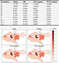
3.2.2. Spatial Mapping
Figure 1 presents relative risk maps of robbery crime in Nairobi County. It is apparent from these map that crime ‘hotspots’ are mainly distributed in the middle, East and Northern areas. The top 10 sub counties with the highest Robbery crime are Kibra, Embakasi central, Embakasi North, Kamukunji, Mathare, Starehe, Makadara, Kasarani, Ruaraka and Langata. The targets of Robbery crimes show that the distribution of robbery cases may have close relations with the distribution of the Sub-counties.
Figure 1. Relative risk map of crime in the county (number of cases per 1000 inhabitants) in Nairobi County during 2011-2018.
Table 2. The results for the main model Parameter estimates from the Model with the least DIC.
Parameter Mean SD 2.5% quant 97.5% quant
k -1.531 0.269 -1.849 -0.800
) 0.008 0.014 -0.019 0.037
)C 0.153 0.056 0.051 0.272
)v 0.007 0.034 -0.062 0.073
)u 0.161 0.031 0.079 0.312
)w 3.979 2.531 -0.553 9.254
m 0.014 0.017 -0.029 0.054
`x.y 0.135 0.038 0.067 0.201
lx.y 1.286 0.173 0.954 1.627
Nx.y 0.231 0.128 0.089 0.514
Figure 2. The corresponding 95% lower (b) and upper (c) credible limits maps, respectively, produced by model 4 (TYPE I).
Figure 2 shows the spatial distribution of Crime in Nairobi County in 2011-2018 based on the best fitting model 4 (TYPE I). This is a map of the corresponding credible interval.
3.3. Related Work
Many studies include only spatial parameters and do not recognize temporal variability. Some studies explore crime hotspots to predict spatial patterns, [15].
Some of them explore the relationships between criminal activity and socio-economic variables, such as education, ethnicity, income level, and unemployment [16].
However, those works do not pay sufficient attention to the spatial-temporal element [17]. Cluster and hotspot detection methods are popular in the spatial-temporal analysis, such as the Knox test and Jacquez test. Johnson et al. provided new insights into the spatial and temporal distribution of repeat victimization in, [18].
Based on the examination result, it can be observed that the rate of repeat victimization was higher than that expected on the basis of statistical likelihood and that the time course of repeat victimization conformed to an exponential model.
Grubesic and Mack explore the utility of statistical measures for identifying and comparing the spatial-temporal footprints of robbery, burglary, and assault, and suggest that these three types of crimes have dramatically different spatial-temporal signatures [19].
4. Conclusion and Recommendation
The study faces some limitations. First, the original data provided by National Police Service solely recorded the exact time of Robbery without considering the condition that robbery happens when people are not at home. Thus, the recorded time is not correct enough, and it is better to use other complementary data to clean the temporal data, such as average time method, rigid temporal search method or aoristic search method. Second, to normalize the variables within the model, the sub-county population is taken into account as the denominator, whereas studies use households as the denominator. Secondary data was used thus obtaining household data was hard. In the future, when the data is collected, both denominators ought to be analyzed and compared. Third, for the Bayesian model during this study, the time period is short, so the temporal impact is taken into account as linear; this can be helpful for determinative the developing trends and impact factors of crime. For long-term fine-granularity data, the Bayesian model ought to take into account the periodical and non-linear trends over time.
Different non-linear models can also be employed to predict crimes, such as neural network model and deep learning model.
Future studies can consider more explicit handling of the prior distribution other than the default Priors specified in R-INLA, [20].
Also exploring spatial clustering of less common causes of crime over time including the ward level this will provide further understanding of how the small scale geographic variation may be spatially patterned across the county. For further work, it could be possible to use additional tests of the multivariate model with different crimes data are recommended
.
Further study can be done to determine factors associated with the distribution and the dynamics of crime in the County while accounting for measurement error that might be present in the covariates.
References
[1] P. Brantingham and P. Brantingham, “Crime pattern theory,” in Environmental criminology and crime analysis, Willan, 2013, pp. 100–116.
[2] S. D. Johnson et al., “Space--time patterns of risk: A cross national assessment of residential burglary victimization,” J. Quant. Criminol., vol. 23, no. 3, pp. 201–219, 2007.
[3] L. E. Cohen and M. Felson, “Social Change and Crime Rate Trends: A Routine Activity Approach (1979),” in Classics in Environmental Criminology, CRC Press, 2016, pp. 203–232. [4] J. Law and R. Haining, “A Bayesian approach to modeling
binary data: The case of high-intensity crime areas,” Geogr. Anal., vol. 36, no. 3, pp. 197–216, 2004.
[5] D. Liu, W. Song, and C. Xiu, “Spatial patterns of violent crimes and neighborhood characteristics in Changchun, China,” Aust. N. Z. J. Criminol., vol. 49, no. 1, pp. 53–72, 2016.
[6] W. J. Zheng, X. Y. Li, and K. Chen, “Bayesian statistics in spatial epidemiology,” Zhejiang da xue xue bao. Yi xue ban= J. Zhejiang Univ. Med. Sci., vol. 37, no. 6, pp. 642–647, 2008. [7] J. Law and M. Quick, “Exploring links between juvenile
offenders and social disorganization at a large map scale: a Bayesian spatial modeling approach,” J. Geogr. Syst., vol. 15, no. 1, pp. 89–113, 2013.
[8] L. W. Mburu and M. Helbich, “Crime risk estimation with a commuter-harmonized ambient population,” Ann. Am. Assoc. Geogr., vol. 106, no. 4, pp. 804–818, 2016.
[9] M. Blangiardo and M. Cameletti, Spatial and spatio-temporal Bayesian models with R-INLA. John Wiley & Sons, 2015. [10] S. J. Rey, E. A. Mack, and J. Koschinsky, “Exploratory
space--time analysis of burglary patterns,” J. Quant. Criminol., vol. 28, no. 3, pp. 509–531, 2012.
[11] J. Besag, “Spatial interaction and the statistical analysis of lattice systems,” J. R. Stat. Soc. Ser. B, pp. 192–236, 1974. [12] J. Besag, J. York, and A. Mollié, “Bayesian image restoration,
with two applications in spatial statistics,” Ann. Inst. Stat. Math., vol. 43, no. 1, pp. 1–20, 1991.
[13] D. J. Spiegelhalter, N. G. Best, B. P. Carlin, and A. Van Der Linde, “Bayesian measures of model complexity and fit,” J. R. Stat. Soc. Ser. B (Statistical Methodol., vol. 64, no. 4, pp. 583– 639, 2002.
[14] T. Hu, X. Ye, L. Duan, and X. Zhu, “Integrating near repeat and social network approaches to analyze crime patterns,” in
2017 25th International Conference on Geoinformatics, 2017, pp. 1–4.
[15] L. W. Sherman and J. E. Eck, “Policing for crime prevention,”
Evidence-based crime Prev., vol. 295, 2002.
[16] I. Ehrlich, “On the relation between education and crime,” in
Education, income, and human behavior, NBER, 1975, pp. 313–338.
[17] T. Almanie, R. Mirza, and E. Lor, “Crime prediction based on crime types and using spatial and temporal criminal hotspots,”
arXiv Prepr. arXiv1508.02050, 2015.
[18] S. D. Johnson, K. Bowers, and A. Hirschfield, “New insights into the spatial and temporal distribution of repeat victimization,” Br. J. Criminol., vol. 37, no. 2, pp. 224–241, 1997.
[19] T. H. Grubesic and E. A. Mack, “Spatio-temporal interaction of urban crime,” J. Quant. Criminol., vol. 24, no. 3, pp. 285– 306, 2008.