www.j-sens-sens-syst.net/6/171/2017/ doi:10.5194/jsss-6-171-2017
© Author(s) 2017. CC Attribution 3.0 License.
Physically based computer graphics for realistic image
formation to simulate optical measurement systems
Max-Gerd Retzlaff1,2, Johannes Hanika1, Jürgen Beyerer2,3, and Carsten Dachsbacher1 1Karlsruhe Institute of Technology (KIT), Institute for Visualization and Data Analysis (IVD),
Computer Graphics Group, Karlsruhe, Germany
2Fraunhofer Institute of Optronics, System Technologies and Image Exploitation (IOSB), Karlsruhe, Germany 3Karlsruhe Institute of Technology (KIT), Institute for Anthropomatics and Robotics,
Vision and Fusion Laboratory (IES), Karlsruhe, Germany
Correspondence to:Max-Gerd Retzlaff ([email protected])
Received: 30 September 2016 – Revised: 21 January 2017 – Accepted: 28 February 2017 – Published: 8 May 2017
Abstract. Physically based image synthesis methods, a research direction in computer graphics (CG), are capa-ble of simulating optical measuring systems in their entirety and thus constitute an interesting approach for the development, simulation, optimization, and validation of such systems. In addition, other CG methods, so-called procedural modeling techniques, can be used to quickly generate large sets of virtual samples and scenes thereof that comprise the same variety as physical testing objects and real scenes (e.g., if digitized sample data are not available or difficult to acquire). Appropriate image synthesis (rendering) techniques result in a realistic image formation for the virtual scenes, considering light sources, material, complex lens systems, and sensor properties, and can be used to evaluate and improve complex measuring systems and automated optical inspection (AOI) systems independent of a physical realization. In this paper, we provide an overview of suitable image synthesis methods and their characteristics, we discuss the challenges for the design and specification of a given measuring situation in order to allow for a reliable simulation and validation, and we describe an image generation pipeline suitable for the evaluation and optimization of measuring and AOI systems.
1 Overview and state of the art in image synthesis
Current physically based image synthesis techniques consti-tute a major leap compared to previously used, mostly phe-nomenological approaches. The simulation of light transport is at the core of physically based image synthesis methods and crucial to generate images that are on par with images made by physical image acquisition systems. Light transport simulation nowadays is almost exclusively computed using Monte Carlo (MC) or Markov chain Monte Carlo (MCMC) methods, which can account for complex light–matter inter-actions and naturally handle spectral emission, absorption, and scattering behavior (measured or derived from models) described by geometric optics. (MC)MC methods can also comprise the simulation of complex lens systems to accu-rately compute the resulting irradiance onto a virtual sensor. Essentially, all (MC)MC rendering methods compute an estimate of the light transport by sampling, that is,
stochasti-cally generating, paths on which light propagates from light sources to sensors, their main difference being the path sam-pling strategy. Until sufficient convergence, the variance of this estimation is apparent as noise in the images. Because of this, even simplistic realizations of these methods are ver-satile and, in principle, capable of achieving the desired, and required, results. However, their application is only practical when an (MC)MC method is used which is well suited for a given scenario; otherwise, the computation time can easily become prohibitively long, even in seemingly simple cases. For example, one would choose different methods for com-puting light transport for complex high-frequency light trans-port phenomena (recognizable by multiple glossy or specular reflection) than for highly scattering media.
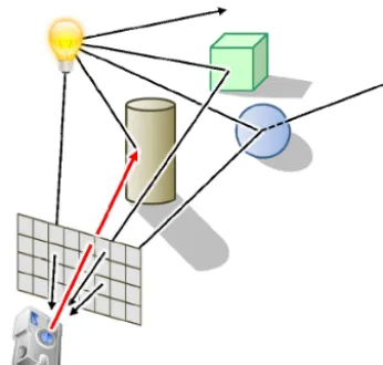
charac-Figure 1.Illustration of basic ray tracing.
teristics, which are strongly linked to the type of light–matter interactions and the geometry configurations occurring in a scene. As such, it is not straightforward for the non-expert to select the appropriate method. For this purpose, we iden-tify light interactions and phenomena constituting different challenges for the image synthesis, and discuss state-of-the-art algorithms, such as, for example, path tracing and bi-directional path tracing (BDPT).
Particular attention has to be paid to the simulation of com-plex lens systems which can increase the computation time by orders of magnitude when implemented naively. We dis-cuss the use of a state-of-the-art approach to efficient render-ing with realistic lenses in the context of measurrender-ing and AOI systems.
2 Image synthesis methods
2.1 Rendering, rasterization, and ray tracing
Hughes et al. (2015) define the term rendering very concisely as referring to the process of integration of the light that ar-rives at each pixel of the image sensor inside a virtual camera in order to compute an image.
There are two major strategies for determining the color of an image pixel: rasterization and ray tracing.
Ray tracing, also sometimes referred to as ray casting, de-termines the visibility of surfaces by tracing rays of light from the virtual view point, that is, the viewer’s eye or the image sensor, to the objects in the scene. The view point rep-resents the center of origin and the image a window on an arbitrary view plane. For each pixel of the image a view ray is sent originating in the view point through the pixel into the scene in order to find an intersection with a surface. By recur-sive application of this ray casting, as illustrated in Fig. 1, one can compute complex light interactions and global illumina-tion, that is, indirect illumination including, among others, reflections and shadows.
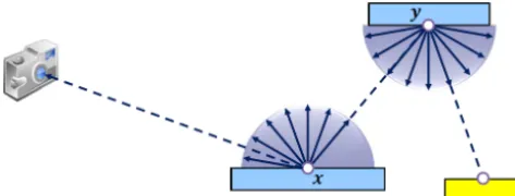
Figure 2.Illustration of the surface interaction at pointx.
Rasterization, on the other hand, projects geometric primi-tives one by one onto the image window. A depth buffer, also called a z-buffer, is utilized to determine the closest and thus visible primitive for each pixel.
Usually, the perspective projection is carried out in three steps. First, the projection transformation, expressed in ho-mogeneous coordinates, is applied. Afterwards, the projec-tive coordinates are dehomogenized by the normalization transformation, mapping the view frustum to the unit cube. The resulting device coordinates can then be mapped to im-age coordinates by discarding the depth component, as is done for orthographic projection.
All primitives can be processed in parallel using a single instruction multiple data (SIMD) approach and minor syn-chronization via the depth buffer. This allows for a very fast pipelined hardware implementation in the form of modern graphics processing units (GPUs).
Simplified, one could say that ray tracing starts with the pixels and then determines ray intersections with the scene geometry, while rasterization starts with the geometry, pro-jecting it onto the image plane. The availability of modern GPUs makes rasterization feasible for interactive real-time application.
2.2 Rendering equation and (Markov chain) Monte Carlo methods
The surface interactions during ray tracing can be described easily, as illustrated in Fig. 2. As we start from the observer, or camera, and try to find paths to the light sources, ray trac-ing essentially considers the backward light transport. This means that for each surface interaction we want to determine the radianceLr(x,ωr), that is, the radiant flux per unit solid
angle emitted or reflected, or transmitted at pointx of the surface in directionωr.
The radiance consists of the light that is emitted in that direction at the surface point,Le(x,ωr), and the light that is
in-Figure 3.Illustration of distributed ray tracing.
coming directionωi we project the solid angle to the surface
and multiply it by the irradianceLi(x,ωi) reaching the point x from directionωi and by a function that describes the
re-flectance, that is, the ratio between irradiance and radiance; cf. Venable and Hsia (1974). Typically, this is a bidirectional reflectance distribution function (BRDF)fr(ωi,x,ωr),
intro-duced by Nicodemus et al. (1977).
All terms combined lead to Eq. (1), also called the render-ing equation, which can be evaluated recursively in order to compute the illumination of a scene (Kajiya, 1986).
Lr(x,ωr)= Z
+
fr(ωi,x,ωr)Li(x,ωi) cosθi dωi (1)
Monte Carlo (MC) methods are a broad class of algo-rithms that numerically evaluate an integral by repeated ran-dom sampling. They are suitable for high-dimensional prob-lems, and as such a good choice to compute the value of the surface integral, as ray tracing is a high-dimensional prob-lem because of multiple reflections and the recursive nature of the rendering equation. The Monte Carlo evaluation of the rendering equation leads to approximation Eq. (2).
Lr(x,ωr)≈
4π N
N−1 X
i=0
fr(ωi,x,ωr)Li(x,ωi) cosθi (2)
Markov chain Monte Carlo (MCMC) methods sample from a probability distribution based on a Markov chain. This allows the construction of a Markov chain with a desired dis-tribution. Also, in the context of rendering, Markov chains make it possible to construct new paths by mutation of ex-isting paths, a fact that is exploited by the Metropolis light transport (MLT) that is described in Sect. 2.3.7.
2.3 Comparison of the suitability of (Markov chain) Monte Carlo rendering techniques for AOI
(MC)MC rendering methods are the predominant way to compute light transport simulations nowadays. In all their diversity, they all share the concept of stochastically creat-ing paths, connectcreat-ing the sensor to the light sources. In this section, we discuss different (MC)MC rendering algorithms and sampling strategies suitable for the simulation of mea-suring situations. As mentioned in introductory Sect. 1 the
Figure 4.Illustration of path tracing.
main differences of these approaches lay in the path sam-pling strategies.
2.3.1 Distributed ray tracing
Ray tracing is the basic approach of casting rays starting from the camera and recursively casting successive rays on reflections. Recursive evaluation of the rendering equation, described in Sect. 2.2, by stochastically sampling the inte-gral leads to distributed ray tracing, introduced by Cook et al. (1984). On each surface interactionN rays are followed, as illustrated in Fig. 3. Sadly, this leads to exponential growth.
Summary. Distributed ray tracing is the straightforward implementation of recursive Monte Carlo evaluation of the rendering equation and as such easy to implement, but more recent methods do not suffer from exponential growth.
2.3.2 Path tracing and next event estimation
Path tracing, introduced by Kajiya (1986), improves upon distributed ray tracing by tracing whole paths from camera to light sources. That is, at every surface interaction only a single new direction is sampled so that each time a single, unambiguous path is generated, and of those paths we cre-ateN for each pixel of the resulting image, as illustrated in Fig. 4.
One problem of ray tracing and path tracing is that a ray or path that does not hit a light source transports no energy and thus has no contribution to the image pixel. At the same time, it is unlikely to hit a light source, in general. To alleviate this problem, optionally, next event estimation (NEE, Kajiya, 1986) can be used to directly sample light sources.
Figure 5.Illustration of light tracing.
Path tracing is able to render caustics1as long as the light source has finite area (i.e., not a point light source). How-ever, the corresponding transport paths are typically sampled with low probability. Thus, path tracing is not well suited for handling such situations.
Summary. Path tracing is easy to implement and suitable if there are no caustics from small light sources and if direct connections to the light sources are possible. Therefore, path tracing is a good candidate for measurement setups where objects are recorded in transmitted light, as here the light source is usually big and always directly visible.
2.3.3 Light tracing
Light tracing, sometimes also referred to as backward ray tracing (Arvo, 1986), is the complementary method of path tracing: as in reality, paths start from the light sources and are followed until they hit the image plane, i.e., the simulated image sensor of the virtual camera. Directions are sampled as is done for path tracing. See Fig. 5.
Next event estimation (NEE) is also optionally possible; in this case, connections to the camera are sampled. However, for light tracing NEE is more problematic in the context of specular surfaces and lens models: specular surfaces limit the reflection path to just one direction. Therefore, it is not pos-sible to sample a different direction that would hit the sensor. Obviously, this is the case when the virtual camera contains a lens system in front of the sensor.
Summary. Like path tracing, light tracing is easy to imple-ment, but it only works well if the light sources directly emit to the surfaces visible to the camera. Otherwise, path tracing (or forward ray tracing) is still employed to determine visual surfaces, as in the next method.
2.3.4 Bi-directional path tracing (BDPT) and multiple importance sampling (MIS)
Bi-directional path tracing, introduced by Lafortune and Willems (1993), is a combination of path and light tracing: the subpaths are constructed starting from both ends,
cam-1A caustic, in optics, is a light bundling pattern created by ob-jects or materials focusing or diverting light by refraction or reflec-tion.
Figure 6. Illustration of bi-directional path tracing (BDPT). (a)“Eye” subpathseistarting at the camera and “light” subpathsli (b)deterministically connect all intermediate paths (nodes).
era and light sources; the intersections of paths with objects of the scene are called nodes. In addition to direct sampling of light sources and the camera, respectively, the intermedi-ate nodes of both path and light tracing subpaths can be de-terministically connected, greatly increasing the number of resulting paths that are likely to transport much energy, and thus have a lot of influence on the illumination of the simu-lated scene. See Fig. 6.
However, increasing the number of possible path combi-nations also means that a technique is necessary to keep the variance of the Monte Carlo estimation low, as the reuse of “light” and “eye” subpaths in the path combinations results in high variance (apparent as high-frequency noise in the re-sulting image) due to correlation between the paths (Popov et al., 2015). Therefore, BDPT usually requires variance re-duction via multiple importance sampling (MIS) to be prac-tical, which unfortunately makes this method non-trivial to implement. MIS, introduced by Veach (1998), is a technique to use multiple sampling methods to evaluate an integral and combine the sample values in a provably good way.
Summary. As mentioned, BDPT is non-trivial to imple-ment because it needs MIS to be practical. BDPT works well in scenes where the deterministic connections are not blocked. This should usually be the case for AOI settings as the measurement setup is usually designed in a way that the objects are well lit and visible to the camera, that is, the ob-jects are visible to both camera and light source.
2.3.5 Many-light methods (variants of BDPT)
Summary. The many-light approach works very well for mostly diffuse scenes and is easy to implement. On the down-side, it has problems with glossy surfaces and is even im-possible to use with specular surfaces; cf. Dachsbacher et al. (2014).
2.3.6 Photon mapping
Photon mapping is the somewhat confusing yet widely used short name for Global Illumination using Photon Maps intro-duced by Jensen (1996). In photon mapping light subpaths are also created, but in this model, the light sources send out photons, i.e., energy units. The node locations, that is, loca-tions where energy impinges on the surface, are recorded in a data structure called a photon map; cf. Fig. 7a.
Afterwards, the scene is rendered with path tracing, but instead of treating the nodes of the light paths as VPLs as in the many-light methods and directly connecting to them with NEE, the photon map is used to compute the illumination. That is, the energy at a surface point is estimated by counting the photons in the local environment of the intersection point (density estimation); cf. Fig. 7b.
Summary. Photon mapping works well with diffuse sur-faces and can render caustics efficiently. For glossy sursur-faces, it (gracefully) degrades to path tracing. Photon mapping can be made robust and has the advantage of producing images with low noise levels, but the density estimation also causes a bias (systematic error); cf. Hachisuka and Jensen (2009).
More extensions and variants to bi-directional methods ex-ist, such as, e.g., Georgiev et al. (2012).
2.3.7 Metropolis light transport (MLT)
The family of the Metropolis light transport methods use the Metropolis–Hastings (MH) algorithm, introduced by Hast-ings (1970), to sample the space of all possible light transport paths, and as such they all are Markov chain Monte Carlo (MCMC) methods.
The basic idea is to first find an important path, that is, a path that transports much energy and thus has high influence on the resulting image, and then to generate similar paths by mutation of the existing important path. This is one of the best strategies for difficult situations, such as, for example, the scene illustrated in Fig. 8, in which the only light source is concealed without any direct connections to the camera.
Numerous variants exist, e.g., sampling in primary space (Kelemen et al., 2002) or in path space (Veach, 1998), as well as modern extensions such as energy redistribution path tracing (ERPT, Cline et al., 2005), manifold exploration (Jakob and Marschner, 2012), half-vector space transport (Kaplanyan et al., 2014), and gradient domain methods (Ket-tunen et al., 2015).
Summary. MLT methods have in common that they are very powerful in exploring difficult light transport phenom-ena (e.g., caustics). However, they have to be initialized
re-Figure 7.Illustration of photon mapping.(a)Light sources send out energy as photons;(b)a density estimation is used to estimate the energy per surface area.
Figure 8.Illustration of Metropolis light transport (MLT) with one important path that reaches the single, concealed light source of this difficult scene, and two mutations of this path.
peatedly with independent MC samplers (e.g., BDPT) and thus rely on those to detect actual occurrences of said light phenomena. In image rendering, this results in images where individual components are rendered with little noise but all occurrences of the light phenomena are only found over time. Also, MLT methods share the property that they are difficult to implement (an exception is Kelemen et al., 2002) and dif-ficult to control.
2.3.8 Realistic lenses
Figure 9.Emission spectrum of a tungsten halogen lamp (Model 3900 by Illumination Technologies, Inc.).
virtual scene and trace rays through it, this leads to very in-efficient rendering, as, for straightforward ray tracing, 95 % of all ray samples, or more, might not leave a real-world lens system and enter the actual scene (Hanika and Dachsbacher, 2014).
The reason for this lies in the fact that straightforward ray or path tracing starts at the sensor and will simply sample lo-cations on the image sensor and directions off the sensor to generate rays, and, thus, many of the rays will hit the hous-ing of the camera or the aperture. This can be avoided by implementing importance sampling (cf. Sect. 2.3.4) of the aperture, that is, by not only sampling the sensor but also points on the aperture. It has to be noted that sampling the aperture is usually not easily possible, as the aperture stop is typically located within the lens system, i.e., between op-tical elements; refer to Hanika and Dachsbacher (2014) and Schrade et al. (2016) for a detailed analysis of this problem.
3 Realistic image formation to simulate AOI systems
3.1 Synthetic images in the context of optical inspection
In Retzlaff et al. (2015) we describe the idea of using com-puter graphics methods to allow systematic and thorough evaluation of automated optical inspection (AOI) systems. Instead of using real objects and acquisition systems, com-puter graphics methods are used to create large virtual sets of samples of test objects and to simulate image acquisition setups. We use procedural modeling techniques to generate virtual objects with varying appearance and properties, mim-icking real objects and sample sets. Physical simulation of rigid bodies is deployed to simulate the placement of virtual objects, and using physically based rendering techniques we create synthetic images. These are used as input to an AOI system instead of physically acquired images. This enables the development, optimization, and evaluation of the image processing and classification steps of an AOI system inde-pendently of a physical realization.
Figure 10.Emission spectrum of a fluorescent ceiling light.
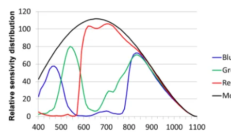
Figure 11.Raw sensor response of the ELiiXA UC4/UC8 line scan camera by e2v.
We demonstrated this approach for shards of glass, as sort-ing glass is one challengsort-ing practical application for AOI. In this paper, we focus on the aspects of image synthesis.
3.2 Synthetic images of glass shards using rasterization
3.2.1 Efficient generation of synthetic glass shards
Retzlaff et al. (2015) describe a procedural model for the gen-eration of virtual 3-D models of glass shards based on an al-gorithm described by Martinet et al. (2004). We modified the algorithm to generate plausible shards with a certain smooth-ing, as waste glass is repeatedly relocated and this leads to rounded edges of the glass shards. In addition to this, our carving volume is smooth to allow fast intersection, while we achieve plausible breaking edges by displacement map-ping of the intersection surfaces using hardware-accelerated tessellation shaders that were introduced in OpenGL 4.0.
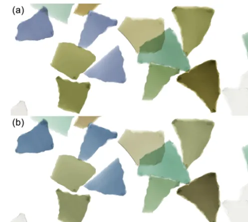
Figure 12.Images rendered in real time using the color matching functions of the CIE 1931 standard colorimetric observer.(a)CIE Illuminant D65;(b)fluorescent illumination of Fig. 10.
3.2.2 Real-time rendering of shard distributions
Our implementation includes real-time rendering of shard distributions by hardware rasterization on the GPU using OpenGL 4.2 (Segal and Akeley, 2012).
As glass is an optically semi-transparent material, a method of transparency rendering is necessary. OpenGL it-self only provides alpha blending that can be used to render transparent materials. But rendering transparency using al-pha blending implies rendering the objects in a sorted order. As sorting for every rendered frame is impractical and even not always possible (e.g., for mutually overlapping objects), order-independent transparency rendering (OIT) techniques have been invented.
Our previous implementation as presented in Retzlaff et al. (2015) used depth peeling (introduced by Cass, 2001), a ro-bust hardware-accelerated OIT method, but meanwhile we replaced this with an implementation of a more powerful OIT technique making use of per-pixel concurrent linked lists (introduced by Yang et al., 2010). OIT rendering us-ing depth peelus-ing can store only a quite limited number of material interactions per image pixel requiring multiple ren-dering passes in case of many interactions. Per-pixel linked list OIT, on the other hand, allows one to store a high num-ber of interactions in a single rendering pass, and the realistic rendering of the breaking edges of glass shards may require a high number of interactions as the edges can be quite rough. As our previous publications Retzlaff et al. (2015) and Ret-zlaff et al. (2014) focus on the generation of realistic virtual objects and scenes based on measured data as well as the methodical procedure of using synthetic images for the
eval-Figure 13.Images rendered in real time using the ELiiXA sensor sensitivity function depicted in Fig. 11.(a)and(b): images illumi-nated as in Fig. 12.
uation of real AOI systems, we had used simplified models of the illumination and image acquisition for the image syn-thesis, e.g., ideal sensors and simplified optical image forma-tion.
Most importantly, we have used RGB rendering. The syn-thesis was therefore reduced to only three values describing red, green, and blue norm stimuli, and could not reproduce spectral effects such as dispersion.
3.2.3 Replicating real image acquisition systems and spectral rendering
Recently, we have enhanced our real-time method to support spectral rendering and to replicate more physical aspects of real image acquisition systems; that is, we now support the simulation of real light sources and sensor responses of real image sensors.
Of course, spectral rendering is especially important in the context of color filters that limit the light spectrum to a nar-row spectral range combined with lighting by a non-uniform illumination.
Figure 14. A synthetic image of procedurally generated virtual glass shards on a diffuse reflecting surface generated by our Monte Carlo rendering framework.
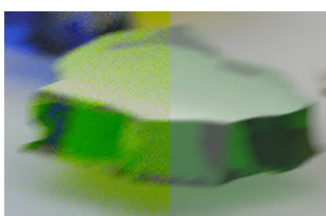
Figure 15.Close-up view of a synthetic shard.(a)Fluorescent illu-mination with bright spectral lines, as depicted in Fig. 10;(b)CIE Standard Illuminant D65. Both images are rendered with 2048 sam-ples per pixel.
In the case of the CIE color matching functions (Smith and Guild, 1931–1932)XY Zcoordinates are computed that describe the color perception of a human being as standard-ized by the CIE 1931 standard colorimetric observer. The
XY Z images can be converted to an RGB working space, such as, for example, the sRGB color space (IEC, 1999), and displayed on a calibrated screen. It thus can serve as a ref-erence image for an expert user designing an AOI setup, as it corresponds to the color impression one would perceive in the simulated viewing conditions; cf. Fig. 12.
Simulation of chromatic adaptation can account for the difference in white reference of the simulated light emission and of the computer screen that is used for viewing.
For our real-time implementation we use a binning ap-proach to spectral rendering. That is, the full spectrum of the visible light is quantized into bins of a certain width; thus, the spectra are approximated by a step function. The spec-tra can either be approximated by equal width bins, which is a sufficient approximation for smooth spectra, or it can be
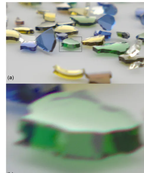
Figure 16.A close-up view of the scene also displayed in Fig. 14 from a different angle.
Figure 17.Double-Gauss lens by Angénieux (1955).
adaptive, as is necessary in the case of illumination with light depicting narrow bright peaks.
3.2.4 Light sources with bright spectral lines and results
While light sources such as incandescent light bulbs or halo-gen lamps have quite smooth spectra, see Fig. 9, the spec-tra of other light sources such as, for example, fluorescent lamps exhibit a number of narrow bright peaks, as depicted in Fig. 10. Such a lighting condition in combination with cer-tain sensors can result in images in which actual spectral dif-ferences cannot be perceived or easily detected anymore.
This can be simulated with spectral rendering, and helps to design an acquisition setup that does not exhibit such prob-lems by choosing a suitable combination of sensor and illu-mination; see Fig. 13 and compare to Fig. 12.
Figure 18.(a)Synthetic image and enlarged section(b)rendered using a thin lens model exhibiting a narrow depth of field (DOF).
3.2.5 Limits of the rasterization approach
While it is possible to add support to rasterization for han-dling more complex light interaction phenomena such as, for example, refraction and dispersion – and has in fact been re-alized in our simulation in the form of a proof of concept implementation for light refraction – one has to accept that rasterization has its limits and at a certain point a ray tracing approach begins to be more feasible, and even more efficient. Support for refraction can be added to a rasterization ap-proach by ray marching, that is, by determining the inter-section point of a ray with a surface not analytically, but by iteratively taking steps along the ray and checking each time whether an intersection has taken place. Obviously, it is much more straightforward to add light refraction to a ray tracer. Dispersion constitutes a similar case. But the afore-mentioned point is surely exceeded when global illumination or simulation of real lens systems including monochromatic and chromatic aberration is asked for. In these cases, a more efficient approach for ray casting than ray marching is called for, as demonstrated in the next part of this section.
Figure 19.Same scene as in Fig. 18 but using a simple achromatic doublet lens (Edmund Optics #NT32-921), exhibiting a less narrow DOF but strong chromatic aberration (color fringing).
3.3 Synthetic images of glass shards using physically based image synthesis
3.3.1 Revised generation of synthetic glass shards
There is a downside to the efficiently generated virtual glass shards that we described in Sect. 3.2.1. In the case of con-siderable displacement, the polygonal mesh might get self-intersections or holes at the transition between intersection surface and original shard surface. Small irregularities can be fixed easily, but bigger defects would require a remeshing of the polygon mesh, slowing down the generation consid-erably. Such erroneous meshes describe surfaces that are not physically possible, and thus present problems for physically based rendering methods. As a result, the law of conservation of energy might get violated at such irregularities.
Therefore, we vouched for a new method of generating shards of broken glass, dropping the requirement of real-time generation and instead introducing a pool of precomputed shard meshes.
Figure 20. Synthetic image using the simple thin lens model as perceived by the CIE 1931 standard colorimetric observer, CIE D65 hemispherical illumination.
Figure 21. Same as in Fig. 20 but using the Double-Gauss lens by Angénieux (1955), also depicted in Fig. 17. The black grid is overlaid to make the difference in distortion easily recognizable.
example of this is the Cell Fracture implementation of the Blender 3-D modeling software by the Blender Foundation.
One notable exception is the method introduced by Ko-rndörfer (2011). It is also based on Voronoi partitioning, but uses a 3-D voxel grid and puts emphasis on achieving a reg-ular quad meshing of the boundary surface. The Voronoi re-gions are not based on the Euclidean distance, but instead on the length of paths in a graph defined by the voxels. The shape of the regions can be controlled by weights of the graph edges. The method already supports random noise edge weights in order to generate irregular, i.e., plausible, surface structures, making it a suitable candidate for our task of generating virtual glass shards.
3.3.2 Physically based rendering and resulting images
Figure 14 shows a scene of the shards generated with the method of Korndörfer (2011) and rendered using our exist-ing Monte Carlo ray tracexist-ing framework supportexist-ing global illumination, that is, a physically based simulation of light transport, which inherently accounts for phenomena such as reflections and shadows. We have chosen path tracing even
Figure 22.Same as in Fig. 21 but detected by the ELiiXA sensor, depicted in Fig. 11.
Figure 23.Same as Fig. 21 but with motion blur.
without NEE for our task, as the AOI setup exhibits a very large light source.
As the ray tracing framework does not use spectral bin-ning but instead supports full spectral rendering with Monte Carlo spectral sampling, it can simulate dispersion. Figure 16 shows a close-up view of the same scene as in Fig. 14 (from a slightly different angle), exhibiting light refraction and chro-matic dispersion.
It is interesting to note that the spectra of the illumination and interacting surfaces might also affect the rendering time or image quality. Uniform sampling of the emission spectrum leads to noisy images in the case of spectra with bright nar-row peaks compared to images using a more homogeneous spectral illumination, as samples fall equally on every part of the spectrum. This is illustrated in Fig. 15.
Importance sampling that results in a higher sampling rate in regions with higher radiance while still being an unbiased estimation can leverage this problem without increasing the sampling count (and thereby increasing the rendering time).
3.3.3 Adding realistic lenses
Figure 24.Double-Gauss lens (Angénieux, 1955), CIE D65 hemi-spherical illumination, CIE standard colorimetric observer.
Figure 25. Same as Fig. 24 but detected by the ELiiXA sensor, depicted in Fig. 11.
a wide range of real-world lenses with only negligible over-head compared to rendering with the thin lens model. Such real-world lenses can consist of dozens of lens elements and an aperture, such as, for example, the Angénieux Double-Gauss lens (cf. Angénieux, 1955, US Patent 2 701 982, ef-fective focal length 100 mm, f/1.1), as depicted in Fig. 17. Still, this approach can accurately compute the lens image and thus be used to simulate flaws and shortcomings of real lens systems.
Figure 18 and Fig. 19 show a group of images of the same scene of glass shards on a diffuse reflecting surface but using different lenses, the thin lens model and a simple achromatic doublet lens (Edmund Optics #NT32-921, modified, effec-tive focal length 129 mm, f/3.3), respeceffec-tively. Both lenses have got different depths of field, and the image by the achro-matic doublet lens exhibits strong chroachro-matic aberration, com-monly referred to as color fringing.
3.3.4 Results and rendering computation times
To conclude this section, we present an overview of render-ings with different lenses as well as color matching and sen-sor sensitivity functions, respectively. Figures 20 to 23 show the scene from a flat angle, while Figs. 24 to 27 show a top
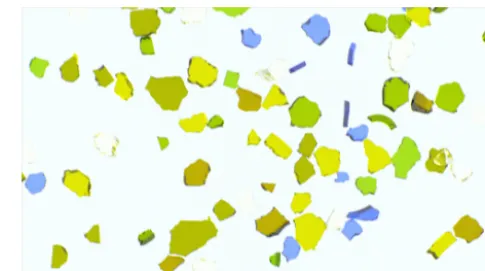
Figure 26.Same as Fig. 24 but with the fluorescent ceiling light of Fig. 10 as strong transmitted light and hemispherical illumination.
Figure 27.Same as Fig. 26 but with the ELiiXA sensor, depicted in Fig. 11.
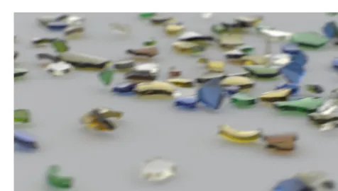
Figure 28.Recorded image of real glass shards obtained by a phys-ical line scan camera (unknown type and sensor) of an AOI image acquisition system (Fraunhofer IOSB, 2012) in transmitted light of a fluorescent illumination, scaled to approximately fit the size of the simulated shards.
ferences, and thus also render images with motion blur of the shards sliding along a sloping surface, as can be seen in Fig. 23.
Tables 1 and 2 contain the computation times for the im-age series Figs. 20 and 23 and Figs. 24 and 27, respectively. All of these images have been rendered at a resolution of 2048×1152 pixels using simple path tracing without next event estimation (NEE) as the rendering method and 2048 samples per pixel on an Intel Xeon E7-8870 CPU with 10 cores (plus Hyper-Threading) at 2.4 GHz.
Please note that we configured our rendering implementa-tion with fixed settings of 2048 samples per pixel regardless of the actual variance to ensure high quality; an adaptive ap-proach could result in shorter rendering times.
The rendering durations are roughly on the same scale, with the exception of Figs. 26 and 27. The scenes of these two images are illuminated with a fluorescent light not only as hemispherical illumination, but also in strong transmit-ted light to simulate the image acquisition conditions of the physical setup.
These exceptions amply demonstrate that path tracing is a well-suited rendering method for applications in transmitted light. The background consists of a large light source that is easy to hit; therefore, direct connections to the light source are easily possible, while in the case of a diffuse surface the paths that hit it need at least one more path segment to reach the hemispherical surrounding light.
Thus, recording images of the shards for this measurement problem in transmitted light is not only an advisable choice for the subsequent image processing task as the shards appear more clearly in the resulting images without casting shadows on the background; see Fig. 27 and compare to Fig. 25. Also, synthetic images of scenes in transmitted light are faster to compute.
4 Conclusion and future work
In summary, we described an entire image synthesis pipeline including all relevant components as well as their efficient and accurate implementation with regard to the simulation and validation of optical measuring systems.
In addition to a real-time image pipeline based on hard-ware rasterization on the GPU, including spectral rendering using a binning approach, we implemented a second pipeline using physically based simulation of light transport including efficient simulation of real-world lens systems. Altogether,
Fig. 21, Angénieux Double-Gauss (DG) 01:27:54 Fig. 22, Angénieux DG + motion blur 01:28:11 Fig. 23, Angénieux DG + ELiiXA sensor 01:27:51
Table 2.Computation times for image series 2: variation in illumi-nation and sensor, Figs. 24 to 27.
Again not optimized for fast computations.
image duration
(hh:mm:ss)
Fig. 24, CIE D65 + CIE observer 01:16:31 Fig. 25, CIE D65 + ELiiXA sensor 01:16:13 Fig. 26, strong Fluorescent + CIE observer 00:41:10 Fig. 27, strong Fluorescent + ELiiXA sensor 00:41:23
this resulted in a realistic simulation of the image formation of an automated optical inspection (AOI) image acquisition system.
Meanwhile, in Retzlaff et al. (2016), we investigated the combination of our synthetic image acquisition (SIA) and machine learning to accelerate design and deployment of AOI systems. We demonstrated that a classifier can be trained using synthetic images, and on physically acquired images this classifier performed on par with a classifier that was trained using physically acquired images.
4.1 Outlook
The simulated image formation now includes measured spec-tral light sources, complex light–matter interaction using measured absorption spectra, and realistic lens systems, and reproduces the sensor response of real sensors. One last thing that is left, is the simulation of sensor noise.
Data availability. No data sets were used in this article.
Competing interests. The authors declare that they have no conflict of interest.
Edited by: M. Fischer
Reviewed by: two anonymous referees
References
Angénieux, P.: Large Aperture Six Component Optical Objective, US Patent 2 701 982, issued 15 February, 1955.
Arvo, J.: Backward Ray Tracing, ACM SIGGRAPH ’86 Course Notes – Developments in Ray Tracing, 259–263, 1986. Cass, E.: Interactive order-independent transparency, NVIDIA
Cor-poration, technical report, 2001.
Cline, D., Talbot, J., and Egbert, P.: Energy Redistribution Path Tracing, ACM Trans. Graph. (TOG) – Proc. of SIGGRAPH 2015, 24, 1186–1195, doi:10.1145/1073204.1073330, 2005. Cook, R. L., Porter, T., and Carpenter, L.: Distributed Ray Tracing,
ACM Proc. of SIGGRAPH ’84 Computer Graphics, 18, 137– 145, doi:10.1145/964965.808590, 1984.
Dachsbacher, C., Kˇrivánek, J., Hašan, M., Arbree, A., Wal-ter, B., and Novák, J.: Scalable Realistic Rendering with Many-Light Methods, Computer Graphics Forum, 33, 88–104, doi:10.1111/cgf.12256, 2014.
Georgiev, I., Kˇrivánek, J., Davidoviˇc, T., and Slusallek, P.: Light transport simulation with vertex connection and merging, ACM Trans. Graph. (TOG) – Proc. of SIGGRAPH Asia 2012, 31, 1– 10, doi:10.1145/2366145.2366211, 2012.
Hachisuka, T. and Jensen, H. W.: Stochastic progressive photon mapping, ACM Trans. Graph. (TOG) – Proc. of SIGGRAPH Asia 2009, 28, 1–8, doi:10.1145/1618452.1618487, 2009. Hanika, J. and Dachsbacher, C.: Efficient Monte Carlo rendering
with realistic lenses, Computer Graphics Forum (Proc. of Euro-graphics), 33, 323–332, doi:10.1111/cgf.12301, 2014.
Hastings, W. K.: Monte Carlo sampling methods using Markov chains and their applications, Biometrika, 57, 97–109, doi:10.1093/biomet/57.1.97, 1970.
Hughes, J. F., van Dam, A., Foley, J. D., and Feiner, S. K.: Computer Graphics: Principles and Practice, 3rd Edn., Addison-Wesley, 2015.
IEC: International Electrotechnical Commission: Multimedia sys-tems and equipment, Colour measurement and management – Part 2-1: Colour management, Default RGB colour space, sRGB, IEC 61966-2-1:1999, iCS codes: 33.160.60, 37.080 – TC 100, 1999.
Jakob, W. and Marschner, S.: Manifold exploration: a Markov Chain Monte Carlo technique for rendering scenes with difficult specular transport, ACM Trans. Graph. (TOG) – Proc. of SIG-GRAPH 2012, 31, 1–13, doi:10.1145/2185520.2185554, 2012. Jensen, H. W.: Global Illumination Using Photon Maps, Proc. of
the Eurographics Workshop on Rendering Techniques ’96, 21– 30, 1996.
Jähne, B.: EMVA 1288 Standard for Machine Vision, Optik & Pho-tonik, 5, 53–54, doi:10.1002/opph.201190082, 2010.
Kajiya, J. T.: The rendering equation, ACM SIGGRAPH Computer Graphics, 20, 143–150, doi:10.1145/15886.15902, 1986. Kaplanyan, A. S., Hanika, J., and Dachsbacher, C.: The
Natural-Constraint Representation of the Path Space for Efficient Light Transport Simulation, ACM Trans. Graph. (TOG) – Proc. of SIG-GRAPH 2014), 33, 1–13, doi:10.1145/2601097.2601108, 2014. Kelemen, C., Szirmay-Kalos, L., Antal, G., and Csonka, F.: A Sim-ple and Robust Mutation Strategy for the Metropolis Light Trans-port Algorithm, Computer Graphics Forum (Proc. of Eurograph-ics), 21, 531–540, doi:10.1111/1467-8659.t01-1-00703, 2002. Keller, A.: Instant Radiosity, ACM Proc. of SIGGRAPH ’97, 49–
56, doi:10.1145/258734.258769, 1997.
Kettunen, M., Manzi, M., Aittala, M., Lehtinen, J., Durand, F., and Zwicker, M.: Gradient-domain path tracing, ACM Trans. Graph. (TOG) – Proc. of SIGGRAPH 2012, 34, 1–13, doi:10.1145/2766997, 2015.
Korndörfer, J.: Interaktive Zerlegung von Festkörpern in Bruch-stücke, diploma thesis, Universität Karlsruhe (TH), 2011. Lafortune, E. P. and Willems, Y. D.: Bi-Directional Path Tracing,
Proc. of Compugraphics ’93, 145–153, 1993.
Martinet, A., Galin, E., Desbenoit, B., and Hakkouche, S.: Procedural modeling of cracks and fractures, Proc. of the Shape Modelling International (Short Paper), 346–349, doi:10.1109/SMI.2004.1314524, 2004.
Nicodemus, F. E., Richmond, J. C., Hsia, J. J., Ginsberg, I. W., and Limperis, T.: Geometric Considerations and Nomenclature for Reflectance, Monograph 161, National Bureau of Standards (US), Washington, D.C., USA, 1977.
Popov, S., Ramamoorthi, R., Durand, F., and Drettakis, G.: Prob-abilistic Connections for Bidirectional Path Tracing, Proc. of the 26st Eurographics Symposium on Rendering (EGSR’15), doi:10.1111/cgf.12680, 2015.
Retzlaff, M.-G., Stabenow, J., and Dachsbacher, C.: Synthetic im-age acquisition and procedural modeling for automated optical inspection (AOI) systems, Forum Bildverarbeitung 2014, 47–59, doi:10.5445/KSP/1000043608, 2014.
Retzlaff, M.-G., Stabenow, J., Beyerer, J., and Dachsbacher, C.: Synthesizing images using parameterized models for automated optical inspection (AOI), tm – Technisches Messen, 82, 251–261, doi:10.1515/teme-2014-0041, 2015.
Retzlaff, M.-G., Richter, M., Längle, T., Beyerer, J., and Dachs-bacher, C.: Combining synthetic image acquisition and machine learning: Accelerated design and deployment of sorting systems, Forum Bildverarbeitung 2016, 49–61, 2016.
Schrade, E., Hanika, J., and Dachsbacher, C.: Sparse high-degree polynomials for wide-angle lenses, Computer Graphics Forum (Proc. Eurographics Symposium on Rendering), 35, 89–97, 2016.
Segal, M. and Akeley, K.: The OpenGL Graphics System: A Spec-ification (Ver. 4.2 (Core Profile) – 27 April 2012), Khronos Group, 2012.