Essays in macroeconomics of debt deleveraging

PhD in Economics (Cycle XXV)

Department of Economics and Finance

Essays in Macroeconomics of

Debt Deleveraging

Candidate: Federica Romei

Supervisor: Prof. Pierpaolo Benigno

Essays in Macroeconomics of Debt Deleveraging

c

COPYRIGHT

2014

Dedicated to my extended family: my mom, my dad, Lorenzo, Enrico, Adriana and

ACKNOWLEDGMENT

This small success has many fathers.

First of all, I would like to express my deepest appreciation to Professor Pierpaolo

Benigno for being such an intellectually generous supervisor. He is one of that kind

of people that, once met, can completely change your life.

Secondly, I would like to thank the Professors of LUISS Economics and Finance

De-partment since they support me during this period of growth.

I am also indebted to all of my friends who gave me the serenity to face this PhD:

among others Valerio and Valerio, Marianna, Peppe, Liliane, Gianna and Peppe,

Luca, Paolo, Alessandra and Andrea, Marta, Francesco and many others.

Lastly, my deepest appreciation goes to my family. I am deeply grateful to my mother,

who taught me to always smile and to my father, who, instead, taught me how to

over-come problems in life. I’d like to especially thank Lorenzo for being the best brother I

can imagine. I am indebted to my aunt Adriana who is a strong support and example

for all my life and to Enrico who is constantly and silently helpful. Finally I’d like to

ABSTRACT

Essays in Macroeconomics of Debt Deleveraging

Federica Romei

This dissertation analyzes, in two chapters, how monetary and fiscal authorities can optimally manage debt reduction episodes.

In the first chapter I show how public debt deleveraging leads to a recession with dif-ferent effects on real interest rates according to the fiscal instruments the government is using to reduce the debt. The fiscal authority should not depress much consump-tion of the agents who hold savings to improve the welfare of the ones who do not have access to financial markets. Moreover speed and timing of public deleveraging depend crucially on the type of instrument the fiscal authority uses to enforce it. Nominal rigidities, in this context, seem to be beneficial for the agents who cannot insure themselves through financial markets.

TABLE OF CONTENTS

ACKNOWLEDGMENT . . . iv

ABSTRACT . . . v

CHAPTER 1 : Need for the Right Speed: Public Debt Deleveraging and the Timing of Austerity . . . . 1

1.1 Introduction . . . 1

1.2 Literature Reviews . . . 3

1.3 Model . . . 4

1.4 Calibration . . . 12

1.5 Benchmark . . . 17

1.6 Nominal Rigidities . . . 26

1.7 Time Span . . . 37

1.8 Conclusions . . . 41

APPENDIX . . . 45

CHAPTER 2 : Debt Deleveraging and the Exchange Rate . . . 47

2.1 Introduction . . . 47

2.2 A simple model . . . 51

2.3 A model with endogenous production and nominal rigidities . . . 66

2.4 Optimal adjustment to international deleveraging . . . 73

2.5 Alternative international transmission mechanisms . . . 82

2.6 Deleveraging and the original sin . . . 90

Introduction

This dissertation analyzes, in two chapters, how monetary and fiscal authorities can optimally manage debt reduction episodes. The first chapter studies what is the optimal public deleveraging speed for a fiscal authority in a closed economy context. The second chapter, written with Prof. Pierpaolo Benigno, instead, considers how a Central Bank should optimally react to an international private deleveraging episode.

More in detail, in the first chapter I study, in a context of heterogenous agents, incomplete markets and closed economy, what is the optimal deleveraging path that a fiscal authority needs to undertake when forced to reduce public debt. I consider a public deleveraging that may occur either through a public expenditure reduction or through an income taxation increase. I analyze, then, what are the consequences, on agents’ welfare, of different speeds of deleveraging and different fiscal instruments. I focus, moreover, part of my analysis on how nominal rigidities interact with public deleveraging.

I find that under taxation experiment real interest rates tend to be very high and this is helpful for the class of agents who holds savings. When, instead, government uses public expenditure to reduce debt, real interest rates are below the steady state: This situation may be beneficial, if economy do not enter a liquidity trap, for the agents who do not participate in financial markets. I also find that, in most cases, agents who do not have access to the financial markets benefit from the presence of downward wages rigidities.

H, as a net borrower and the other country, F, as a net saver and we shock the economy raising the cost of borrowing. Finally we assume the presence of a unique Central Bank (or equivalently two cooperative Central Banks) that maximizes the welfare of economy as a whole. The question we address is how the Central Bank can manage optimally this deleveraging episode.

We find that there are three channels through which the global economy can absorb the private deleveraging costs. The first is the reduction of the real interest rate of country H, the one who reduces his debt. The second is the expenditure-switching channel, namely a depreciation of the currency of country H in order to steal part of global demand. Unfortunately, movements in the nominal exchange rate lead to inefficient movements in the terms of trade, increasing the economy’s welfare costs. The third mechanism that the Central Bank can use is the reduction of the nominal interest rate of the country F who is a net saver. According to the degree of home bias and the elasticity of substitution between goods produced in country H and F, Central Bank mixes the three channels to react optimally to the deleveraging shock.

CHAPTER 1

Need for the Right Speed:

Public Debt Deleveraging and the Timing of

Austerity

1.1. Introduction

Many countries have experienced in recent years a significant increase in the size of their public debt. While in some countries public debt increased largely as a conse-quence of the financial crisis, notably in the United States, in others, debt was already significantly high at the onset of the crisis. As some Eurozone economies struggled to refinance their debt, those who received assistance packages from institutions such as the International Monetary Fund or the European Central Bank were asked to implement plans to reduce their stock of liabilities. Even economies that did not receive assistance are now facing the question of how to deleverage. Remarkably, this episode of public debt deleveraging is set to occur after an unprecedented recession, whose effects have been felt differently according to agents’ position in the wealth distribution.

markets.

In my model, the government can use public expenditure or distortionary income taxation to deleverage. Agents differ with respect to their possibility of accessing financial markets: Only a subset of consumers can borrow or lend to smooth their consumption. In this context, public sector deleveraging has strong redistributional effects. Indeed, a large public debt implies high taxes (or low public expenditure) for all agents, while interest payments only accrue to those holding public bonds. High government debt is then a net transfer of wealth from the consumers who cannot trade financial assets to the ones who can. The timing of deleveraging and the fiscal instrument chosen to perform it are therefore not inconsequential in this context.

The choice of instrument through which the fiscal authority will reduce debt is impor-tant to determine dynamics of aggregate variables and agents’ welfare. A reduction in public expenditure or an increase in distortionary taxation will lead to different types of recessions, with different effects on interest rates. In the first case, the real interest rate prevailing in the economy will fall. The government and agents who do not participate in financial markets will gain from low real interest rates. When the fiscal authority uses taxes to reduce the debt, instead, interest rates rise significantly. Consumers who hold public bonds will be the ones to benefit from this situation.

1.2. Literature Reviews

My research is closely related to two different strands of the literature: one that has focused on private debt deleveraging and its interaction with monetary policy, and another one on optimal fiscal policy under commitment.

Papers in the literature on private debt deleveraging typically model such an event as an exogenous shock then analyzing the impact of different monetary policies in this context. Some recent papers, such as Guerrieri and Lorenzoni (2010), Krugman and Eggertsson (2012) or Philippon and Midrigan (2011) have studied debt deleveraging in a closed economy. Others, among which Fornaro (2012) Cook and Devereux (2012) and Benigno and Romei (2012), have focused on the consequences of private debt deleveraging in an international context. I depart from this literature in two way: I analyze a public debt deleveraging and I study how the deleveraging path impacts on agents welfare.

aims to understand how a government can react optimally to a shock. This chapter, instead, aims to understand, what is the optimal government-induced shock on the economy.

My paper is close to the work of R¨ohrs and Winter (2014). They analyze what are the consequences of a public debt reduction under heterogenous agents, market incompleteness under flexible prices on aggregate welfare . My research differ in that I focus on the optimal deleveraging speed and on its interaction with nominal rigidities.

1.3. Model

1.3.1. Consumers

I consider a closed economy inhabited by two types of agents, that I call Savers and Hand-to-Mouth. There is a continuum of measure 1−χ of Savers and a continuum of measure χ of Hand-to-Mouth. There is no uncertainty, so all agents have perfect foresight. Following Weil (1992), Savers differ with respect to the type of financial markets they can have access to. Hand-to-Mouth are endowed at birth with one unity of equity in all the firms in the economy. They cannot hold any other type of financial assets. Savers, instead, are not only endowed with the same amount of equity in firms that borrowers have, but they are also able to trade in riskless, one-period, non-contingent bonds. Access to financial markets allows Savers to choose how to optimally allocate their consumption intertemporally. Hand-to-Mouth agents, on the other hand, are forced to solve a static problem in each period.

economy. Savers, on the other hand, proxy for richer consumers who hold financial assets in their portfolio.

Savers and Hand-to-Mouth have identical preferences over streams of consumpion,C and government-provided services, G. Moreover, they enjoy leisure and they supply hours of labor l to firms in the economy. Agents’ lifetime utility is:

∞ X

t=0

βtU(C_tj, Gt, ltj) f or j ={H, S} (1.1)

where U(.) is concave, twice differentiable and satisfies the Inada condition.

I assume that C and Gare bundles of goods

C = Z 1

0

c(i)−1di

−1

and

G= Z 1

0

g(i)−1di

−1

,

where c(i) andg(i) are private and public consumption of a generic good iproduced in the economy. I assume the presence of a continuum of measure one of goods, which are imperfect substitute with an elasticity of intratemporal substitution equal to in both aggregators.

Savers and Hand-to-Mouth to firms two different varieties of labor. Every agent supplies labor to all the firms. Total labor supply of each agent is then:

lH =

Z 1

0

lH(i)di lS =

Z 1

0

lS(i)di

(S). Since agents are indiffernt across firms to which they supply labor, an agent of type H (S) will receive the same wage WH (WS) from all firms.

Savers trade one-period riskless bond,bs

t in unit of consumption good that pays a real

interest rate, rt. Hand-to-Mouth, instead, consume profits distributed by firms and

their labor income in each period. Their respective budget constraints are as follows:

C_tS =WS,tlS,t(1−τt)−bSt +

bS_t+1 1 +rt

+$t (1.2)

and

C_tH =WH,tlH,t(1−τt) +$t (1.3)

where$ are profits paid by each firm and τt is a proportional income tax charged by

the fiscal authority.

Real interest rate is determined by the Fisher equation:

(1 +rt) =

(1 +it)

Πt+1

where it is the nominal interest rate at time t and Πt+1 is the gross inflation at time t+1. Since the nominal interest rate cannot be negative, the real rate must be greater than the inverse of inflation, i.e.:

(1 +rt)≥

1 Πt+1

(1.4)

decide consumption and labor supply, according to the first order condition:

Ul(cHt , Gt, lH,t)

Uc(cHt , Gt, lH,t)

=−WH,t(1−τt) (1.5)

Savers, on the other hand, decide how much to save as well as consumption and hours supplied, maximizing (1.1) subject to (1.2):

Uc(cSt, Gt, lS,t) =β(1 +rt)Uc(cSt+t, Gt+1, lS,t+1) (1.6)

Ul(cSt, Gt, lS,t)

Uc(cSt, Gt, lS,t)

=−WS,t(1−τt) (1.7)

Savers smooth consumption intertemporally according to their Euler equation. Note that since Savers are the only type of agent that can optimally allocate their in-tertemporal pattern of consumption, their behavior will critically affect the price of the bond and the interest rate.

1.3.2. Firms

The economy is populated by a continuum of identical firms of measure one. Each firm has access to the following technology

y(i) = L(i)ω = (LS(i)αSLH(i)αH) ω

(1.8)

allowing them to transform a mix of two different types of labor inputs, LS and LH

into output of a differentiated good.

Total labor hired by each firm is a Cobb-Douglas aggregator of labor supplied by each type of agent, with αS +αH = 1 and αS > αH to capture positive correlation

opereate under decreasing return to scale, so that ω <1.

Every firm

min

LS(i),LH(i)WSLS(i) +WHLH(i) (1.9) subject to

y(i)≤y¯

From the optimization problem above, I derive

WSLS(i)

αS

= WHLH(i) αH

=W L(i)

where the aggregate real wage W is defined as:

W = (kWαS

S W

αH H )

where k≡ 1 αS

αS 1 αH

αH .

Each firm i, competing under monopolistic competition, faces a demand schedule of the type:

y(i) =

p(i) P

−

[C+G] =

p(i) P

−

Y (1.10)

where p(i) is the price set by firm i and P is the price aggregator defined as:

P = Z 1

0

p(i)1−di 1−1

is measured in units of aggregate final output, i.e.:

φ(pt(i), pt−1(i), Yt) =

φ 2

pt(i)

pt−1(i) ¯Π −1

2 Yt.

where ¯Π is steady state inflation andφ >0 determines the degree of nominal rigidity.

Firms maximize the present discounted sum of their profits:

$(i)t=

∞ X

t=0 βtλt

pt(i)

Pt

yt(i)−Wt(i)Lt(i)−φ(pt(i), pt−1(i), Yt)

(1.11)

subject to (1.8) and (1.10), where λt ≡(χUc(cHt , Gt, ltH) + (1−χ)Uc(cSt, Gt, lSt)) is a

weighted average of agents’ specific stochastic discount factors. I can exploit the fact that every firm faces the same cost as well as the same demand schedule to drop the i index. First order condition for profits is as follows:

Wt=

ω µY

1−1 ω

t +

φω (Πt−

¯ Π)ΠtY

1−1 ω

t −β

λt+1 λt

φω

(Πt+1− ¯

Π)Πt+1Yt+1Y −1

ω

t (1.12)

where µ ≡

−1 is the markup and Πt ≡ Pt

Pt−1 is the gross inflation rate. Output ,

Yt, increases if either aggregate real costs decrease, Wt, if current inflation increases

or if future inflation will decrease. From this equation it is possible to derive the standard positively sloped AS curve, since firms will supply more output whenever prices increase.

account the presence of this rigidity.

This friction is expressed as follows:

WS,t ≥ψWS,t−1Πt WH,t ≥ψWH,t−1Πt (1.13)

where ψ ∈ [0,1] is a measure of wage rigidity: ψ = 0 means that wages are free to move, while ψ = 1 leads to completely rigid nominal wage. I assume that the parameter ψ is identical for both labor markets.

Labor markets, whenever condition (1.13) is binding, will determine hours worked by the demand side, only. This will generate some involuntary unemployment due to high cost in that labor market. To summarize, when wages are free to move labor markets will clear, otherwise there will be an excessive supply of labor hours.

(LH,t−χlH,t) (WH,t −ψWH,t−1Πt) = 0 (1.14)

and

(LS,t−(1−χ)lS,t) (WS,t −ψWS,t−1Πt) = 0 (1.15)

1.3.3. Government and Central Bank

The government provides Gt units of non-rival consumption good in every period.

Public expenditure is financed either by charging taxes on labor income or by issuing a bond in term of consumption good, BG

t whose return, also denominated in units of

consumption good, is the real interest rate, rt. Government budget constraint is :

τt(WtSl S t +W

H t l

H

t ) = Gt+

BG t+1 (1 +rt)

−BG_t (1.16)

Since a fraction of the population is not able to optimally smooth consumption, the fiscal authority, by borrowing and saving, can positively affect the welfare of such agents.

The objective of the Central Bank is to maintain inflation on target whenever possi-ble. The Central Bank keeps the nominal interest rate at zero whenever the desired nominal interest is negative.

   

  

Πt= ¯Π if it≥0

it= 0 Otherwise

(1.17)

1.3.4. Market Clearing Condition

Goods and financial markets clear, i.e.:

(1−χ)C_tS+χC_tH +Gt=Yt (1.18)

Labor markets clear only if the constraint (1.13) is not binding. Hence:

(LH,t−χlH,t) (WH,t −ψWH,t−1Πt) = 0

and

(LS,t−(1−χ)lS,t) (WS,t −ψWS,t−1Πt) = 0

1.3.5. Equilibrium

Given a sequence of taxes, public expenditure and nominal interest rates {τt, Gt}∞t=0

an equilibrium is a sequence of prices {rt,Πt, Wt, WtS, WtH}

∞

t=0 and allocations,

{CS

t, CtH, LSt, LHt , lSt, ltH, bst, Yt} such that:

• Given prices, Savers maximize (1.1) subject to (1.2) and Hand-to-Mouth maxi-mize (1.1) subject to (1.3) ;

• Every firm maximizes (1.11) subject to (1.8) and (1.10) ;

• Goods, financial and labor markets clear, (1.18), (1.18), (1.14) and (1.15);

• Government Budget Constraint is satisfied, (1.16);

• Central Bank targets the inflation, (1.17);

1.4. Calibration

1.4.1. Quantitative Results

Kan-ishka and Surico (2011), among others. These authors, highlight, in particular, that a variable determining different effects of fiscal changes is tightness of borrowing con-straints, captured in this paper by the inability to borrow of Hand-to-Mouth agents.

I consider a scenario under which that the fiscal authority is forced to bring down its debt from an high level, BH_{, to a low one, B}L _{in a determined time span. Such a}

debt reduction can be rationalized in several ways. For example, this path may be imposed by the existence of a supranational authority or by international investors willing to charge an infinite cost to the economy if at timeT debt is not at the target, BL_.

Note that infinte paths are available to the fiscal authority to converge to the new steady state. I restrict my analysis to the class of monotonic decreasing deleveraging paths. This seems consistent with casual empirical evidence: as Southern European economies implemented austerity measures in response to the recent sovereign debt crisis, the proposed plans for public borrowing generally implied a mononotonically decreasing path for public debt.

I model the path of deleveraging as:

B_tG =B_tH + (B_tL−B_tH)

t T

J B

where I assume a strictly positive J B. Figure 1 show that J B is a measure of the speed of the public deleverage. A J B < 1 determines a convex deleveraging path (fast) while with a J B >1 deleveraging is a concave process (slow).

Pareto weights on the heterogeneous agents that populate this economy.

The following proposition shows how, under certain conditions on agents’ value func-tions, studying individual consumers’ welfare allows us to exclude a given set of Pareto dominated policies. This will allow us, on the other hand, to state that the optimal policy for the economy as a whole will belong to the complement of this set.

I define the welfare function as:

W e(J B) = ∞ X

t=0

βt{aW eH(J B) + (1−a)W eS(J B)}

where W eH(J B) and W eS(J B) are the Hand-to-Mouth and Savers value function,

respectively, as a function ofJ B anda is a generic weight that can take any value in the interval [0,1]. I define J BH _{and J B}S_{, respectively as}

J Bk= arg max_{J B}W ek(J B) k ={S, H}.

Moreover, I define J BW _as:

J BW = arg max_{J B}W e(J B)

Proposition 1 If agents’ value functions are continuous, twice differentiable and concave in J B, with J BS _{< J B}H _{(J B}H _{< J B}S_{), then the J B}W _{that maximize W}

for a generic a∈[0,1] will lie in the interval [J BS_{, J B}H_{] ([J B}H_{, J B}S_{]). All the J B} who do not belong to this interval are Pareto dominated.

Proof is in appendix A.

to include either reductions in government expenditure or increases in tax rates, but not both. Obviously, fiscal authorities in the real world may adopt a combination of these. However, this restriction allows to consider separately the effects of different types of fiscal contractions.

0 2 4 6 8 10 12

90 91 92 93 94 95 96 97 98 99 100

Quarters

D

eb

t

o

n

G

D

P

%

JB=0.2

JB=1

JB=2.5

1.4.2. Calibration

The model is calibrated quarterly. I use a global method to take into account non linearities that may arise from the Zero Lower Bound and downward nominal wage rigidities. Preferences take the following functional form:

U(cj, G, lj) = (c

j ψ_G1−ψ₎1−ρ

1−ρ −

lj(1+η)

(1 +η) f or j={S, H}

where I set ψ = .9 and ρ = η = 2 in line with the literature1_{. I assume that 80%} of consumers are Savers - χ = .2. I set αS equal to 0.8 such that individual labor

income is identical for the Savers and for t Hand-to-Mouth2_{. I set ω, the parameter} governing decreasing return to scale to equal 0.9.

I set real rate in line with literature at 2.5% and the steady state gross inflation equal to 1. I assume that the elasticity of substitution among the different varieties, , is equal to 8 such that the markup is 1.14.

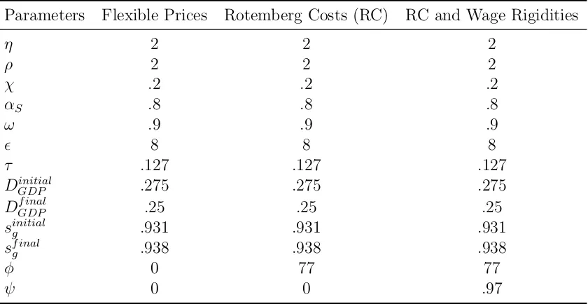
I set tax in initial and final steady state to match the median payroll tax in US, τ = .127 . In 2013 US debt to GDP held by the public but not by the Federal Reserve System equalled 55%. More than half was held by foreign investors. Hence, I set the debt to GDP at yearly basis at 27.5% and I decrease this to 25% during the exercise.

In all the exercises, I set public expenditure as a share of GDP,sg, to equal.931 in the

initial steady state and equal to .938 in the final steady state. When debt reduction occurs through income tax I move in the first quartersg from.931 to .938. The time

span of deleveraging,T, is equal to 4 quarters.

1_{De Walque, Smets and Wouters (2005)}

2_{From firms’ cost minimization} (1−χ)

α WSlS = χ

Parameters Flexible Prices Rotemberg Costs (RC) RC and Wage Rigidities

η 2 2 2

ρ 2 2 2

χ .2 .2 .2

αS .8 .8 .8

ω .9 .9 .9

8 8 8

τ .127 .127 .127

Dinitial

GDP .275 .275 .275

Df inal_GDP .25 .25 .25

sinitial

g .931 .931 .931

sf inal

g .938 .938 .938

φ 0 77 77

ψ 0 0 .97

Table 1: This table shows parameters values used for calibration under different the exer-cises of the chapter/paper.

1.5. Benchmark

In this section I assume that φ = ψ = 0, so that prices are perfectly flexible, and that the nominal interest rate can go below zero, so that the constraint (1.17) does not hold. This formulation is helpful to understand the main mechanism behind the model and it will be the benchmark for all other exercises.

1.5.1. Public Expenditure

It is important to note that, the less gradual the process of debt reduction, the more sizable will be the drop in the real rate. As a result, Hand-to-Mouth prefer a debt reduction that occurs in as few quarters as possible. Moreover, they would like deleverage to take place as soon as possible. The explanation is straightforward: assume that most of the debt reduction occurs in the last quarter. Knowing this, Savers will be willing to move resources from the future to the present. This will put an upward pressure on the real rate before deleveraging has been undertaken. The government would then pay a high interest rate on a large stock of debt. As a consequence, Hand-to-Mouth consumers dislike such a deleveraging path and they would prefer the debt reduction to occur as soon as possible.

As shown in Figure 2 , under this public expenditure experiment, Hand-to-Mouth prefer an extremely fast deleverage. The fiscal authority severely reduces public ex-penditure in the first quarter. Output collapses since firms face a drop in demand. Savers, being forced to save less, experience a boom consumption. The real rate de-creases, reducing financing costs for the government. Note that, despite the aggressive policy stance, debt to GDP do not fall immediately due to the recession.

Movements in the real rate will also drive Savers’ choice of optimal deleveraging path. Since they want to avoid an extreme drop in the real interst rate, they prefer, as Figure 2 shows, a relatively slow and smooth reduction of debt. Savers, knowing that they will experience a consumption boom in the last quarters, are willing to dissave in the first quarters. The real rate falls in the last quarter but, in the preceding periods, it will be relatively high. The economy will experience a prolonged output recession, mostly due to the fall in Hand-to-Mouth consumption and government expenditure. Debt to GDP will converge slowly to the new steady state.

prevents large fluctuations in real variables.

0 1 2 3 4 5

0 5

10 C

S

%

0 1 2 3 4 5

−1 −0.5

0 C

H

%

0 1 2 3 4 5

−2 −1 0

lS

%

0 1 2 3 4 5

0 2

4 l

H

%

0 1 2 3 4 5

−1 −0.5

0 Y

%

0 1 2 3 4 5

−10 0

10 r

%

0 1 2 3 4 5

24 26 28

BG D P

%

Quarters

S

Ht m

0 1 2 3 4 5

−40 −20

0 G

%

Quarters

1.5.2. Taxation

I consider now an experiment in which the fiscal authority raises income tax to finance reduction in debt.

As before, independently on the speed of deleverage, the economy will experience an output recession. Differently from before, however, the negative demand shock, will be only indirectly created by the government. Agents, facing high distortionary taxes, are poorer. As they consume less, output is depressed.

On the other hand, during the debt reduction, the real interest rate will now increase. Savers, indeed, face a reduction in their after-tax labor income. Having access to the financial market, they are then willing to borrow, putting upward pressure on the real rate. The government then has to deleverage when financing costs are high. Tax pressure on the agents needs to increase further to finance the debt reduction. Consumption falls by more, further increasing the pressure on real rate. The economy enters a vicious circle of deep output recession and high interest rate.

Note that, despite the fall in own private consumption and public expenditure, Savers gain during the transition, independently on the deleveraging speed. Their financial income increases, allowing them to enjoy more leisure when their wage is lowered by distortionary taxation.

Hand-to-Mouth, under this experiment would prefer instead a slow debt reduction, as they want to reduce upward pressure on the real rate. As shown by Figure 3, the economy enters a long output recession. The real rate is close to the steady state, spiking in the last quarter. Compared to the previous case, Hand-to-Mouth consumption decreases by more, while labor supply increases due to the high real interest rate.

0 1 2 3 4 5 −2

0

2 C

S

%

0 1 2 3 4 5

−20 0

20 C

H

%

0 1 2 3 4 5

−10 0 10

lS

%

0 1 2 3 4 5

0

5 l

H

%

0 1 2 3 4 5

−5 0

5 Y

%

0 1 2 3 4 5

0 10

20 r

%

0 1 2 3 4 5

20 25 30

BG D P

%

Quarters

S

Ht m

0 1 2 3 4 5

10 20

30 τ

%

Quarters

1.5.3. Consumption Equivalent

In order to compare welfare under the two fiscal experiments I compute the consump-tion equivalent,ce as:

∞ X

t=0

βtU(C_tj, Gt, ltj) =

U(Cj −cj_e, Gj, lj)

1−β j ={S, H}

where the right hand side is utility for consumerj computed along the simulations and Cj_{, G and l}

j are consumption, public expenditure and labor, respectively, computed

at the final steady state for consumer of typej. Following Lucas (1987), I define con-sumption equivalent as the decrease in steady-state concon-sumption that makes agents indifferent between a constant consumption path and the time-varying one achieved in the simulation. Under this definition, a positive consumption equivalent amounts to a welfare cost while a negative consumption equivalent amounts to a welfare gain.

In Figure 4 I plot consumption equivalent as a percentage share of final steady state consumption for Hand-to-Mouth (first panel) and Savers (second panel) as a function of the speed of deleveraging, J B. Solid line refers to deleveraging achieved via a reduction in public expenditure, while the solid line refers to the increase in taxes experiment. 3

In this flexible price setup, Hand-to-Mouth lose during the debt reduction, indepen-dently of the speed of deleveraging. On the other hand, Savers may gain or lose depending on the speed. The Figure shows how some deleveraging paths are Pareto dominated by others: for example, under tax experiment for whichJ B >1.75, where 1.75 is the minimum consumption equivalent achievable by the Hand-to-Mouth,

wel-3_{Note that the consumption equivalent is a continuos and convex function in the debt reduction}

fare of both agents would improve by choosing a lower J B .

Limiting the analysis to the interval of debt reduction speedsJ B that are not Pareto dominated, Hand-to-Mouth lose less, in term of welfare, from a deleveraging achieved by a fall in public expenditure than from one achieved by an increase in taxes. The main difference between the two experiments is in the behavior of the real interest rate. Hand-to-Mouth, once they internalize the government budget constraint, are net borrowers. As a consequence, they dislike high real interest rates. Moreover, under the tax experiment, the economy enters a deeper recession than under the public expenditure case. Hand-to-Mouth agents, having no access to the financial market, will be more exposed to the cost of the recession.

On the other hand, Savers have strong preferences for deleveraging via taxation. Indeed, oppositely than Hand-to-Mouth, they hold public bonds, thus benefitting from high real interest rates.

0 2 4 6 8 10 12 14 16 18 20 0.06 0.08 0.1 0.12 0.14 0.16 Hand-to-Mouth C o n su m p ti o n E q u iv a le n t %

0 2 4 6 8 10 12 14 16 18 20

−0.02 −0.01 0 0.01 0.02 C o n su m p ti o n E q u iv a le n t

% Save rs

J B

P. E . Tax e s

1.6. Nominal Rigidities

Some of the results in the previous section hinge fundamentally on the assumption of perfect price flexibility. Figure 2 shows that the real rate needs to go below zero whenever the government reduces his public expenditure in order to deleverage. Neg-ative real interest rates prevent real variables from experiencing large fluctuations. While negative real interest rates have been observed in reality, this is generally not the case for nominal interest rates, placing a lower bound on real rates too. I assume then in this section that the Central Bank is constrained by the presence of the Zero Lower Bound on nominal interest rates (eq. (1.17)).

In the previous formulation, additionally, firms were able to absorb negative demand shocks by cutting nominal wages. Again, this might not be feasible since nominal wage are downwardly rigid in the data. To capture such features in the context of my experiment, I consider now positive Rotemberg adjustment costs and occasionally binding downward wage rigidities. In subsection 1.6.1 I assume the presence of Rotemberg costs without wage rigidities. Under this circumstance, I will analyze only how simulations under public expenditure change, since this is the only instance in which the real rate goes below zero. In subsection 1.6.2 I assume the presence of both Rotemberg costs and nominal wage rigidities.

1.6.1. Rotemberg costs and the Zero Lower Bound

In this section and the following, I introduce the presence of a sizeable price rigidity4_.

pay a higher real interest rate on public debt and, as a consequence, public expenditure will have to decrease more. Moreover, the fall in public expenditure will further depress output. Tax revenues fall and public expenditure decrease once more. Under the Zero Lower Bound, the economy enters a vicious cycle of low public expenditure and low output since, as shown by a strand of the literature5_{, the public expenditure} multiplier may be greater than one in this setup.

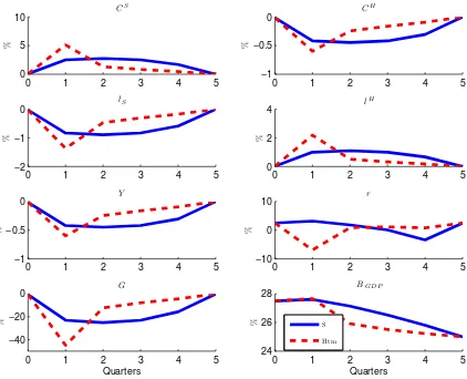
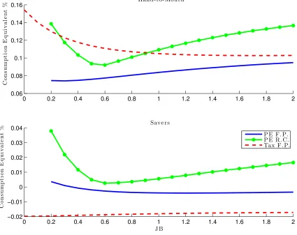
Note that, as Figure 5 shows, preferences of Savers and Hand-to-Mouth converge. As explained in the sections above, under flexible prices, extreme deleveraging paths -very slow or -very fast - are the ones in which real interest rates fall more to clear the market. Consequently, if the Zero Lower Bound binds, these will be the costliest combinations for the economy. The Pareto optimal interval of values of J B shrinks substantially, as extreme choices have become very unfavourable. Due to the larger fall of productive government expenditure, Hand-to-Mouth consumers experience a welfare loss that is higher than the one under flexible prices. Savers switch from a welfare gain under flexible prices to a welfare loss.

It is now ambiguous whether Hand-to-Mouth prefers a debt reduction through taxa-tion or public expenditure. For deleveraging paths of intermediate speed, as before, Hand-to-Mouth prefers a reduction in public expenditure. For extreme cases, however, as the Zero Lower Bound kicks in, he prefers the adjustment to take place through taxes. As deleveraging that takes place via expenditure becomes more costly, Savers, who preferred a taxation driven adjustment already, have their relative preferences unchanged.

Inroducing the Zero Lower Bound, then, has a significant effect on agents’ welfare and their choices. A fiscal authority who wishes to contract public expenditure to reduce

debt needs to consider the possibility of entering a detrimental liquidity trap. Hence, depending on deleveraging speed, it may be the case that distortionary taxation is a more suitable policy instrument to achieve the desired result.

0 0.2 0.4 0.6 0.8 1 1.2 1.4 1.6 1.8 2

0.06 0.08 0.1 0.12 0.14 0.16 Hand-to-Mouth C o n su m p ti o n E q u iv a le n t %

0 0.2 0.4 0.6 0.8 1 1.2 1.4 1.6 1.8 2

−0.02 −0.01 0 0.01 0.02 0.03

0.04 Save rs

C o n su m p ti o n E q u iv a le n t % J B

P E F. P. P E R. C. Tax F. P.

1.6.2. Wage Rigidities

Recently, a big strand of the literature, like Benigno and Ricci (2011), Schmitt-Groh´e and Ur´ıbe(2011) and Calvo et al. (2013) among others, has analyzed how nominal downward wage rigidities affect economies both in the short and in the long run. Downward wage rigidities, under certain condition, can magnify recessions : Since firms are not able to decrease their costs, they will decrease their production. In the next subsections I will study how the presence of downward wage rigidities together with Rotemberg costs, changes agents’ welfare and preferences. In equation (1.13) I set ψ, the parameter governing the extent of wage rigidity, to equal 0.97. As I will show, downward nominal wage rigidities have a different impact according to the type of recession the economy is facing.

Public Expenditure

To understand results under downward wage rigidities, it is useful to consider how labor reacts during deleveraging under flexible prices. In this circumstance, when debt reduction occurs, output falls and firms demand less labor. Savers, on one hand, experiencing a boom in consumption, will enjoy more leisure. On the other hand, Hand-to-Mouth, experiencing a negative shock on their consumption and public expenditure, increase their labor supply. In equilibrium, then, Hand-to-Mouth wage falls more than Savers’ one. Adding Rotemberg costs does not change labor markets dynamics but, as I explained above, the economy is lead into a liquidity trap.

variables while aggregate variables remain largely unchanged due to the liquidity trap. High labor market costs, indeed, exert an upward pressure on nominal prices, making deflation less severe. Nominal interest rate will be still at zero. Consequently, the real interest rate will either remain unchanged or slightly fall, either leaving unaffected or mildly dampening the extent of the recession.

Downward wage rigidities under a liquidity trap, then, will be a transfer of resources from Savers - who work more- to Hand-to-Mouth - who work less. This result critically depends on the presence of the liquidity trap. As detailed by Eggertsson (2010), when the Zero Lower Bound binds, the ”paradox of flexibility” may hold. This is a situation in which flexible prices are more detrimental for the economy than rigid ones. Hence, in this case, nominal rigidities, especially regarding wages, will not exacerbate the cost of deleveraging on the economy.

As Figure 9 shows, downward wage rigidities reduce welfare costs for Hand-to-Mouth agents, while increasing costs for Savers independently on the speed of debt reduction. It is still ambiguous whether Hand-to-Mouth prefer public expenditure or taxation. Indeed, for a fast deleveraging, they bear a lower welfare cost under public expendi-ture, while, for a slow one, they are better off in the case of increase taxation. Agents’ preferences regarding the speed of deleveraging under public expenditure remain, in-stead, unchanged.

could be the case, in a more accurate analysis, that, ex-post, unemployed Hand-to-mouth would be worse off under nominal wage rigidities. Indeed, the presence of these kind of rigidities, may decrease the probability to become employed once a worker is unemployed. This analysis is left for future research.

0 2 4 6 8 10

0 2 4 6 CS %

0 2 4 6 8 10

−2 −1 0 1 CH %

0 2 4 6 8 10

−2 −1 0 1 lS %

0 2 4 6 8 10

0 0.5 1 1.5 lH %

0 2 4 6 8 10

−2 −1 0 1 WS %

0 2 4 6 8 10

−6 −4 −2 0 WH %

0 2 4 6 8 10

0 1 2

3 r

%

Q u a r t er s

0 2 4 6 8 10

−2 −1 0 1 Y %

Q u a r t er s

R . C. W . R .

0 2 4 6 8 10 0 2 4 6 CS %

0 2 4 6 8 10

−2 −1 0 1 CH %

0 2 4 6 8 10

−4 −2 0 2 lS %

0 2 4 6 8 10

−1 0 1 2 lH %

0 2 4 6 8 10

−4 −2 0 2 WS %

0 2 4 6 8 10

−6 −4 −2 0 WH %

0 2 4 6 8 10

0 1 2

3 r

%

Q u a r t er s

0 2 4 6 8 10

−2 −1 0

1 Y

%

Q u a r t er s

R . C. W . R .

Taxation

When a government is deleveraging through taxation, downward wage rigidities, whenever binding, are welfare decreasing. Since nominal wages increase, prices in-creases too, exerting upward pressure on the inflation rate. As a consequence, the Central Bank needs to raise the nominal interest rate and the government, paying an higher real interest rate,has to raise taxes. The recession is, then, deeper than under flexible prices. Differently than under the public expenditure experiment, aggregate variables dynamics change significantly with the introduction of nominal wage rigidi-ties, as Figure 1.13 shows. There Savers optimal deleveraging path under flexible prices is compared with the same deleveraging path under wage rigidities.

Note that downward wage rigidities bind whenever the deleveraging speed is too slow or too fast, as shown in Figure 9. Under these combinations, indeed, real interest rates are very high in equilibrium, as explained in section 1.5.2. The higher interest rates, the higher will be the shock on Hand-to-Mouth consumption and, as a result, the higher will be their increase in labor supply. Consequently, under these debt reduction paths, nominal wages fall substantially. Under flexible prices Savers were the ones who preferred extreme debt deleveraging combinations, as they gained from high real interest rates. This beneficial effect is now dampened by the cost introduced by downward wage rigidities. They will prefer, then, the fastest debt reduction path under which the downward wage rigidity does not bind. Hand-to-Mouth, on the other hand, still find optimal the same debt reduction path they chose under flexible prices.

reduction. If deleveraging is fast they prefer public expenditure, if instead it is slow they prefer taxation.

0 2 4 6 8 10 −5 0 5 CS %

0 2 4 6 8 10

−40 −20 0 20 CH %

0 2 4 6 8 10

−20 −10 0 10 lS %

0 2 4 6 8 10

−10 −5 0 5 lH %

0 2 4 6 8 10

−2 0 2 4 WS %

0 2 4 6 8 10

−10 −5 0

WH

%

0 2 4 6 8 10

0 20 40

60 r

%

Q u a r t er s

0 2 4 6 8 10

−20 −10 0

10 Y

%

Q u a r t er s

F . P. W . R .

0 0.2 0.4 0.6 0.8 1 1.2 1.4 1.6 1.8 2 0.05 0.1 0.15 0.2 0.25 Hand-to-Mouth C o n su m p ti o n E q u iv a le n t %

0 0.2 0.4 0.6 0.8 1 1.2 1.4 1.6 1.8 2 −0.02 −0.01 0 0.01 0.02 0.03

0.04 Save rs

C o n su m p ti o n E q u iv a le n t % J B

P E F. P. P E R. C. P E W. R. Tax F. P. Tax W. R.

1.7. Time Span

Lastly I analyze whether and how the debt reduction time span changes agents’ wel-fare. On one hand a longer time span decreases the size of the per-quarter shock, on the other hand it takes more time for agents to achieve a constant level of consump-tion. To address this question I focus on the Pareto dominant interval of deleveraging paths. As all this combinations are Pareto optimal, the maximum achievable by one agent corresponds to the minimum for the other. Figures 10 and 11 show the min-imum and maxmin-imum consumption equivalent6 achievable by each type of agent as function of debt deleveraging time span,T. Figure 10 shows, for the public expendi-ture experiment, the relevant Pareto intervals under flexible prices, Rotemberg costs and downward wage rigidities (with Rotemberg costs). Figure 11 corresponds to the taxation experiment.

Under public expenditure Savers gain slightly from an increase in the time span. Nevertheless, the magnitude of the gain is negligible. The effect of increasing the time span on Hand-to-mouth welfare is instead significant and counterintuitive. As T increases, Hand-to-Mouth welfare worsens, in both best and worst case scenarios. Indeed, with a shorter time span, as the shock on output demand is larger, real interest rates tend to be lower. The higher will be the time span, the higher will be the real interest rate and the lower will be Hand-to-Mouth welfare. Moreover, Figure 10 also shows that the Pareto interval widens, meaning that the higher the time span, the more Savers and Hand-to-Mouth preferences will differ. Then, as T increases, the variability of outcomes increases for the Hand-to-Mouth.

Under the taxation experiment, Savers are, again, indifferent to the time span, both

under flexible prices and under downward wage rigidities. Hand-to-Mouth, on the other hand , experience an improvement in their welfare, as the time span increases . When a government reduces debt through taxation, interest rate are higher. As T increases, the per-quarter-shock is smaller and, as a consequence, interest rates increase less. Hand-to-Mouth, then, experience a welfare gain with an higher T.

5 10 15 −15 −10 −5 0 5

x 10−3

S a v e r s c . e . % T

5 10 15 −15

−10 −5 0 5

x 10−3

T

5 10 15 −15

−10 −5 0 5

x 10−3

T

5 10 15 0.075 0.08 0.085 0.09 0.095 0.1 H a n d -t o -M o u t h c . e . %

F l e x i b l e P r i c e s

5 10 15 0.075 0.08 0.085 0.09 0.095 0.1

R o t e m b e r g C o s t s

5 10 15 0.075 0.08 0.085 0.09 0.095 0.1

R C a n d Wa g e R i

4 6 8 10 12 14 16 −0.02 −0.0195 −0.019 −0.0185 −0.018 −0.0175 −0.017 S a v e r s c . e . % T

4 6 8 10 12 14 16

−0.02 −0.0195 −0.019 −0.0185 −0.018 −0.0175 −0.017 T

4 6 8 10 12 14 16

0.09 0.1 0.11 0.12 0.13 0.14 0.15 0.16 H a n d -t o -M o u t h c . e . %

F l e x i b l e P r i c e s

4 6 8 10 12 14 16

0.09 0.1 0.11 0.12 0.13 0.14 0.15 0.16

R C a n d Wa g e R i g .

1.8. Conclusions

I analyze welfare implications of different paths of public deleveraging on different types of agents. I find that, in a context of heterogenous agents and incomplete markets, the speed of deleveraging is not inconsequential for agents’ welfare.

Deleveraging through income taxation leads to a recession with high real interest rates. In this situation, agents, who hold public debt prefer extreme deleveraging paths, while consumers who do not participate in the financial markets prefer slower one. An economy choosing, instead, to reduce public debt using public expenditure faces the risk to enter a liquidity trap. Under this circumstance, independently of their participation in financial markets, agents prefer the path that minimizes the fall in public expenditure.

Moreover, I find that downward wage rigidities are always detrimental for the agents who participate in financial market. These rigidities, acting as a sort of insurance in bad times, on the other hand, are helpful for the financial constrained.

Bibliography

[1] Aiyagari , S. Rao, Albert Marcet, Thomas J. Sargent and Juha Seppala (2002), “Optimal Taxation without State-Contingent Debt,”NBER Working Papers No. 19470.

[2] Bhandari, Anmol, David Evans, Mikhail Golosov and Thomas J. Sargent (2013), “Taxes, Debts, and Redistributions with Aggregate Shocks,” Journal of Political Economy ,110(6): 1220-1254.

[3] Benigno, Pierpaolo and Luca Antonio Ricci (2011), “The Inflation-Output Trade-Off with Downward Wage Rigidities,” American Economic Review,101(4):1436-66.

[4] Benigno, Pierpaolo and Federica Romei (2012), “Debt Deleveraging and the Exchange Rate,” forthcoming Journal of International Economics.

[5] Calvo, Guillermo, Fabrizio Coricelli and Pablo Ottonello (2012), “Jobless Recov-eries During Financial Crises: Is Inflation the Way Out?” NBER Working Paper No.19683.

[6] Cook, David and Michael B. Devereux ( 2011). Sharing the burden: monetary and fiscal responses to a world liquidity trap. Unpublished manuscript, University of British Columbia.

[8] Eggertsson, Gauti (2009), “What fiscal policy is effective at zero interest rates?”

Federal Reserve Bank of New York Staff Reports.

[9] Eggertsson, Gauti (2010), “Paradox of toil,” Federal Reserve Bank of New York Staff Reports.

[10] Eggertsson, Gauti and Paul Krugman (2012), “Debt, Deleveraging, and the Liq-uidity Trap: A Fisher-Minsky-Koo Approach,” The Quarterly Journal of Eco-nomics 127(3): 1469-1513.

[11] Fornaro, Luca (2012), “International Debt Deleveraging,” unpublished manuscript, London School of Economics.

[12] Fornaro, Luca (2013), “Debt Deleveraging, Debt Relief and Liquidity Traps,” unpublished manuscript, London School of Economics.

[13] Guerrieri, Veronica and Guido Lorenzoni (2010), “Credit Crisis, Precautionary Savings and the Liquidity Trap,” unpublished manuscript, MIT.

[14] Guiso, Luigi, Michael Haliassos and Tullio Jappelli (2000),“Household Portfolios: An International Comparison,”,CSEF Working Papers.

[15] Kanishka, Misra and Surico, Paolo (2011),“Heterogeneous Responses and Aggre-gate Impact of the 2001 Income Tax Rebates,”,C.E.P.R. Discussion Papers No. 8306.

[16] Karantounias, Anastasios (2013), “Optimal fiscal policy with recursive prefer-ences, ” 2012 Meeting Papers.

Policy in an Economy without Capital,” Journal of Monetary Economics, 12(1) : 55-94.

[18] Lucas, Robert E., Jr. (1987), “Models of Business Cycles,” JBasil Blackwell, New York.

[19] Philippon, Thomas and Virgiliu Midrigan (2011), “Household Leverage and The Recession,” NBER Working Papers No 16965.

[20] R¨ohrs, Sigrid and Christoph Winter (2014), “Reducing Government Debt in Presence of Inequality,” Unpublished Manuscript.

[21] Rotemberg, Julio J. (1982), “Sticky prices in the united states,” Journal of Po-litical Economy 90:1187-1211.

[22] Schmitt-Groh´e, Stephanie and Martin Ur´ıbe (2011), “Pegs and Pain,” NBER Working Paper No. 16847.

[23] Weil, Philippe (1992), “Hand-to-Mouth consumers and asset prices, ” European Economic Review, 36(2-3): 575-583.

APPENDIX

Appendix A

Proposition 2 If agents’ value functions are continuos, twice differentiable and con-cave in J B with J BS < J BH (J BH < J BS), then the J BW that maximize W for a

generic a∈[0,1], will lie in the interval [J BS, J BH]([J BH, J BS]). All the J B those do not belong to this interval are Pareto dominated.

Proof. Being an argmax J BW _{satisfies the following condition:}

W e0(J BW) =aW e0_H(J BW) + (1−a)W e0_S(J BW) = 0 (1.20)

whereW e0(.),W e0_H(.) andW e0_S(.) are the first derivatives ofW e(.),W eH(.) andW eS(.)

with respect to J B.

By contradiction assume thatJ BW _{< J B}S_{, thenW e}0

H(J BW)>0 andW e

0

S(J BW)>

0, then condition (1.20) will not be met. Again by contradiction assume thatJ BW _>

Appendix B

Agents Flexible Prices Rotemberg Costs (RC) RC and Wage Rigidities Taxation

Hand-to-Mouth 1.75 1.75 1.75

Savers 0 0 0.7

Public Expenditure

Hand-to-Mouth 0.3 0.6 0.5

Savers 1.2 0.6 0.6

CHAPTER 2

Debt Deleveraging and the Exchange Rate

1

2.1. Introduction

The decade leading up to the financial crisis was marked by divergences and disequilib-ria. Global imbalances have been at the center of the debate, with several economists warning against the unsustainability of the US external position. The euro area has experienced internal current account divergences, producing an enormous accumula-tion of debt. The crisis was most severe in the economies that had piled up too much private or public debt in one form or another. It is still being debated whether the divergences of the past actually caused the crisis or merely reflected other underlining problems.2 _{In any case, the general tendency is for the crisis-ridden countries to} re-duce debt. In this deleveraging process, exchange-rate policies have been often placed under scrutiny, as in the case between US and China or in reference to the choice of irrevocably fixing exchange rates in the eurozone.

Debt deleveraging raises interesting questions on macroeconomic adjustment. A re-cent literature, spurred by the works of Eggertsson and Krugman (2012), Guerrieri and Lorenzoni (2010) and Philippon and Midrigan (2011), has studied the mechanism of adjustment to debt deleveraging but in closed economies. So far the international

1_{I wrote this chapter with Prof. Pierpaolo Benigno.}

consequences have been neglected. This is a gap that this work aims at filling given the importance of the aforementioned debate on global and European imbalances. There are two main contributions of this paper. First, to understand the interna-tional transmission mechanism of debt deleveraging. Second, to discuss its welfare consequences by asking how monetary and exchange-rate policies should be designed to better accommodate from a global perspective the ensuing macroeconomic adjust-ment.3

The transmission mechanism of a reduction in one country’s external debt presents some familiar features with that of the old transfer problem, as discussed among others in Keynes (1929). Deleveraging forces debtor countries to cut spending sharply and depresses demand. Spending should increase in the rest of the world. But international relative prices might not be immune to the adjustment.4 _{If the fall in} demand is sharper for domestic goods, which is the case when there is home bias in consumption, the excess supply of these goods globally lowers their prices relative to foreign prices and expands overall demand for them, thus easing the depressive impact of deleveraging. These changes in relative prices are achieved by depreciation of the deleveraging country’s currency. In the longer run, a country that has paid down part of its debt is richer than at first, since there is less debt to serve, so the demand for domestic goods is relatively higher. The exchange rate swings from short-term depreciation to appreciation in the long run. But, without home bias, deleveraging does not produce any movement in the exchange rate in both the short and long run.

Following the propagation mechanism described above, we could be tempted to

con-3_{It should be noted that none of the papers of Eggertsson and Krugman (2012), Guerrieri and}

Lorenzoni (2010) and Philippon and Midrigan (2011) deals with the welfare consequences of debt deleveraging.

4_{In the current debate on the unwinding of global imbalances, Feldstein (2011) and Krugman}

clude that the exchange rate, and other international relative prices, should move substantially to mitigate the costs of deleveraging, but only when there is home-bias in goods consumption. Otherwise a fixed-exchange rate would be desirable. However, this conclusion is completely misleading if viewed from the perspective of a benevo-lent planner maximizing welfare in the global economy. Indeed, this planner dislikes any large variations of consumption, output and relative prices and would prefer, instead, to accommodate the adjustment in a smoother way. This is not feasible and interesting trade-offs emerge between output, consumption and terms-of-trade stabilization.

There are three available channels through which the global economy can absorb in a better way a deleveraging shock. The first channel is a pure domestic one, already emphasized by the closed-economy literature as in Eggertsson and Krugman (2012). The real interest rate in the deleveraging country should fall to reduce its borrowing costs while adjusting to a lower level of debt. To this end, a policy in which the interest rate of the deleverager stays at the zero-lower bound is desirable. The other two channels have instead an international dimension: the expenditure-switching channel and the fall in the real interest rate in the non-deleveraging countries.

The expenditure-switching channel driven by movements of the exchange rate is clearly desirable from a global perspective to the extent that can mitigate the output recession in the deleveraging country by shifting the burden of adjustment to other countries. However, it leads to costs in terms of movements in the terms of trade, which are unjustified by efficient shocks.5 _{In general, the benevolent planner dislikes} large variations of the exchange rate and other international relative prices. Indeed, when the expenditure-switching effect is stronger because domestic and foreign goods

are more substitute, the optimal movements in the exchange rate are small. On the contrary, when the expenditure-switching effect is too weak, a depreciation of the currency can adversely reduce the real income of the country, making it even more poor. Also in this case, the exchange rate should not depreciate much.

A fall in the real interest rate in the non-deleveraging countries is also desirable to the extent that can raise foreign consumption to offset the recession in the deleverager.6 However, the rise in consumption in the rest of the world is also unjustified by efficient shocks and therefore brings inefficiencies. When the expenditure-switching channel is more effective, the fall in the foreign real rate is less needed. On the contrary, when the expenditure-switching channel is weak, the real rate should fall substantially in the rest of the world. In this case a global liquidity trap can be desirable as when countries are more open to trade.

There are some earlier works related to our framework. Obstfeld and Rogoff (2001, 2005, 2007) also studied the exchange-rate implications of a sudden improvement in one country’s current account balance, conducting some comparative-static ex-periments without analyzing the welfare consequences. Our focus here is on dy-namic adjustment, on the role of monetary policy taking into account the zero lower bound and on optimal monetary policy from a global perspective. Policies at the zero lower bound, in an open economy, have been explored by Svensson (2001, 2003), Jeanne (2009) and Fujiwara et al. (2010, 2011), but in different models without debt deleveraging. There is also substantial literature on open economies analyzing credit-constrained economies and the implications of relaxing or restricting credit access for the equilibrium economy: see among others Aghion et al. (2001), Aoki et al. (2010) and Mendoza (2010) and more recently Devereux and Yetman (2010). In an

open-economy model, Cook and Devereux (2011) have studied the optimal response to preferences’ shocks which bring one country to the zero lower bound while appre-ciating its currency. In a recent work, Fornaro (2012) studies also international debt deleveraging emphasizing similar mechanisms of adjustment as in our framework. He is not concerned with welfare implications but analyzes mostly the occurrence of liq-uidity traps under a monetary union. Bhattarai et al. (2013) study instead optimal monetary policy in a currency-area model with financial frictions.

This paper is organized as follows. Section 2.2 describes a deleveraging shock in a simple two-country open-economy endowment model. Section 2.3 extends the basic model to include nominal rigidities and endogenous output. Section 2.4 discusses optimal policy from a global perspective. Section 2.5 performs some robustness anal-ysis by varying the degrees of home bias and the elasticity of substitution between traded goods. Section 2.6 analyzes the case in which debt deleveraging concerns debt denominated in foreign currency. Section 2.7 concludes. An online appendix reports the main equations of the model and the solution method.7

2.2. A simple model

We adopt a simple two-country endowment economy to study how debt deleveraging in one country spreads to the rest of the world economy. The two countries are Home, denoted byH, and Foreign, denoted byF. Each country has an endowment of a good. The two goods, H and F respectively, are traded frictionlessly. The representative agent of country H maximizes utility from consumption

∞ X

t=0

βtu(Ct),

where β is the discount factor with 0< β < 1. The consumption index C is a Cobb-Douglas aggregator of the consumption of the two goods, CH (denoting Home goods)

and CF (denoting Foreign goods):

C=

CH

α

α

CF

1−α 1−α

, (2.1)

where 0 < α < 1 represents the share of consumption of goods H in the overall consumption basket, for a consumer of countryH.Given the prices for the two goods, PH and PF, expressed in the currency of country H, the consumption-based price

index of the Home country, P, is

P =P_HαP_F1−α.

Consumers in the Foreign country maximize their utility from consumption

∞ X

t=0

βtu(C_t∗),

where the consumption basket C∗ is:

C∗ =

C_H∗ 1−α∗

1−α∗ C_F∗

α∗ α∗

, (2.2)

and nowα∗, with 0< α∗ <1, is the weight given to goodsF.The general price index in country F is:

P∗ =P_H∗(1−α∗)P_F∗α∗,

The two goods are traded with no friction, and the law of one price holds

PF =SPF∗, PH =SPH∗,

where S is the nominal exchange rate, defined as units of Home currency per unit of Foreign currency. Preferences are biased towards domestic goods under the assump-tion thatα =α∗ >1/2. In this case, our model generates deviations from purchasing power parity (PPP), in which the real exchange rate (Q) is proportional to the terms of trade T =PF/PH

Q= SP ∗ P =

PH

PF

1−2α

=T2α−1. (2.3)

Given preferences and prices, demands for the goods are:

CH =α

PH

P −1

C, CF = (1−α)

PF

P −1

C,

C_H∗ = (1−α∗)

P_H∗ P∗

−1

C∗, C_F∗ =α∗

P_F∗ P∗

−1 C∗.

Consumers in the Home country receive in every periodt an endowmentYH,t of good

H, which they can sell at the pricePH,t; they consume a bundle Ct of goodsH andF

at pricePt; borrow or lend resourcesDt+1/(1 +it), in units of currency of countryH,

and pay back or receive the face value of the funds lent in the previous periodDt. A

positive value for Ddenotes nominal debt. Dis the only asset traded internationally and 1 +iis the one-period risk-free gross nominal interest rate on domestic currency.8

8_{Nominal bonds allow for meaningful asset trading even when consumption baskets are different}

As a result, the flow budget constraint for consumers in the Home country is:

PtCt=PH,tYH,t+

Dt+1 1 +it

−Dt. (2.4)

There is a limit on the amount of real debt that the agent can take in each period

Dt

Pt

≤k, (2.5)

wherek >0. Similar constraints have been used in other open-economy models, such as Aoki et al. (2010), Devereux and Yetman (2010) and Mendoza (2010). They are justified in terms of the guarantees that international creditors require when borrowers have limited commitment. As in Eggertsson and Krugman (2012), we do not model the source of this constraint but interpret it as the maximum size of the debt that can be considered safe and that international investors are willing to lend to country H at each point in time. A change in this limit –in particular its reduction over time– constitutes the debt-deleveraging experiment analyzed here.9 This drop can happen just for a change in confidence triggered by an internal banking or financial crisis –not modelled here– so that international investors are more reluctant to lend to country H. In the equilibrium that we are going to analyze, consumers in country H will be at the corner and (2.5) limits their borrowing capacity.

Looking now at country F, the flow budget constraint is:

P_t∗C_t∗ =P_F,t∗ Y_F,t∗ + D ∗

t+1 St(1 +it)

− D ∗

t

St

, (2.6)

where Y_F,t∗ represents the endowment of good F and D∗_t the holding of nominal debt

in units of currency H. Consumers in country F face a similar borrowing limit in units of their consumption basket:

D∗_t P_t∗St

≤k∗, (2.7)

for a positivek∗.In the equilibrium that we are going to analyze, consumers in country F will be creditors in international markets and the limit in (2.7) is not binding.

The optimal intertemporal allocation of consumption in country H is governed by the following Euler equation:

Uc(Ct)≥β(1 +rt)Uc(Ct+1), (2.8)

where the home-country real interest rate is defined as

1 +rt ≡

(1 +it)Pt

Pt+1 .

Similarly, the Euler equation for consumers in country F is:

Uc(Ct∗)≥β(1 +r

∗

t)Uc(Ct∗+1), (2.9)

where the foreign-country real interest rate is connected to the home-country real rate through

(1 +rt) = (1 +r∗t)

Qt+1 Qt

.

Equilibrium in goods and asset markets implies

YH,t=Tt1−α[αCt+ (1−α)QtCt∗], (2.10)

Y_F,t∗ =T_t−α[(1−α)Ct+αQtCt∗], (2.11)

Dt+D∗t = 0. (2.12)

Combining the equilibrium in the goods market, the terms of trade can be written as

Tt =

YH,t

Y_F,t∗

(1−α)Ct+αQtCt∗

αCt+ (1−α)QtCt∗

, (2.13)

while the real exchange rate follows from Qt =Tt2α−1.

Two results can be read directly from equation (2.13). First, a relative abundance of Home over Foreign goods lowers Home prices relative to the Foreign (expressed in the same currency), worsening the Home terms of trade and depreciating its real exchange rate. If prices of goods are rigid in the endowment currency or if the monetary authority strictly targets the domestic price level, this corresponds to a nominal depreciation. Under these assumptions, in what follows, we use terms of trade, real and nominal exchange rates interchangeably.10

Second, and more important, home bias in consumption is crucial in order for delever-aging to influence the exchange rate. In fact, if preferences are identical across coun-tries (α= 1/2), the terms of trade are independent of the distribution of wealth and

10_{In the model with nominal rigidities the decomposition of the terms of trade into prices and}

just proportional to the ratio of the endowments of the two goods.11 _{Instead, when} there is home bias, the distribution of wealth and debt across countries can also affect relative prices through the demand channel. Imagine that deleveraging in the Home country reduces Home consumption. Since Home consumers demand more of their own goods, the fall in Home consumption depresses the demand for Home goods more than that for Foreign goods. The price of the Home goods relative to Foreign falls, worsening the Home terms of trade and depreciating the Home currency. In these cases, exchange rate management is a factor in the debt-deleveraging transmission mechanism.

2.2.1. Steady state

A deleveraging shock produced by a lowering of the debt limitk in the Home country requires some time to be absorbed. In this section we abstract from the adjustment process and compare the initial and final steady-state equilibria. We start from an initial steady state in which the distribution of wealth is such that consumers in the home country come up against their borrowing limit. This is a feasible choice because the initial distribution of wealth is indeterminate given that agents in the two countries share the same discount factor. Steady-state Home and Foreign real interest rates (¯r and ¯r∗) are tied to the subjective discount factorβ

(1 + ¯r∗) = (1 + ¯r) = 1

β, (2.14)

where an upper bar denotes variables at their steady-state levels. Debt in the Home country is at the borrowing limit (2.5), and the steady-state level of consumption

11_{This is a standard result that depends on the assumption of Cobb-Douglas preferences, as in}

follows from the budget constraint (2.4)

¯

C = ¯Tα−1Y¯H −(1−β)k. (2.15)

Combining (2.3), (2.6) and (2.12) consumption in the Foreign country is given by

¯

QC¯∗ = ¯TαY¯_F∗+ (1−β)k. (2.16)

The steady-state terms of trade can be simply obtained by appropriately incorporat-ing (2.15) and (2.16) into (2.13)

¯ T =

¯ YH

¯ Y_F∗

1 + (1−β)

2α−1 1−α

k ¯ Tα−1_Y¯

H

. (2.17)

2.2.2. Adjustment to a deleveraging shock in country H

We now study the dynamic adjustment to a deleveraging shock that hits country H. Let us say that for exogenous reasons, there is a fall in the maximum amount of external debt that can be considered risk-free: the debt ceilingk drops from khigh to

klow. The adjustment takes place in two periods, the short run and the long run.

In the long run, denoted by a bar, the results of section (2.2.1) apply. The real interest rate follows from (2.14) while ¯T, ¯C,C¯∗ and ¯Qsolve equations (2.3), (2.13), (2.15) and (2.16). With respect to the initial steady state, consumption in the Home country will be higher in the long run, since there is less d