R E S E A R C H
Open Access
Micro-crack detection of multicrystalline solar cells
featuring an improved anisotropic diffusion filter
and image segmentation technique
Said Amirul Anwar and Mohd Zaid Abdullah
*Abstract
This paper presents an algorithm for the detection of micro-crack defects in the multicrystalline solar cells. This detection goal is very challenging due to the presence of various types of image anomalies like dislocation clusters, grain boundaries, and other artifacts due to the spurious discontinuities in the gray levels. In this work, an algorithm featuring an improved anisotropic diffusion filter and advanced image segmentation technique is proposed. The methods and procedures are assessed using 600 electroluminescence images, comprising 313 intact and 287 defected samples. Results indicate that the methods and procedures can accurately detect micro-crack in solar cells with sensitivity, specificity, and accuracy averaging at 97%, 80%, and 88%, respectively.
Keywords:Micro-crack detection; Multicrystalline solar cell; Image segmentation; Anisotropic diffusion; Angular radial transform; Support vector machine
1. Introduction
The increasing demand for solar electrical energy has multiplied the need for photovoltaic (PV) arrays. As the major component of the PV array, the demand for solar cells has also increased. This demand has translated into an increased production of solar cells in recent years. Depending on the materials used in manufacturing, solar cells can be divided into two major types. They are (i) monocrystalline and (ii) multicrystalline silicones. Due to low manufacturing and processing cost of the multi-crystalline silicon, this material is generally more preferred in the production of the solar wafer or PV module. There is great potential for the automation in solar cell industry because millions of solar cells are manufactured daily worldwide. According to recent statistics, the growth rate of the solar PV module reached a record high in 2011, generating more than US$93 billion in revenue with multicrystalline cells constituting more than 50% of the world production [1]. Although many operations in the PV industry have been automated, the inspection and grading processes continue to be based on manual or semi-manual efforts.
Finished solar cells are occasionally found to be defective or faulty. The defects fall into two groups: (i) intrinsic and (ii) extrinsic. Grain boundaries are an example of intrinsic defect, while micro-cracks belong to the second category. The former type of defects diminish the short-circuit current of the cell, and this leads to loss in the efficiency. The latter defects form a class of cracks that are entirely invisible to the naked eye. With dimensions smaller than 30 μm [2], this type of defect can only be visualized elec-tronically like using the electroluminescence (EL) technique and high-resolution cameras.
In practice, there are various shapes and sizes of micro-cracks in a solar cell depending on how they are formed. For example a line-shaped micro-crack is caused by scratches, and it generally occurs during cell fabrication [3]. This type of defect can also be due to wafer sawing or laser cutting, which propagates and causes the detachment or internal breakage of the grainy materials within the solar cells [4]. In contrast, star-shaped micro-crack is formed due to a sharp point impact which induces several line cracks with a tendency to cross each other [5]. There are other types of micro-crack defects, but these two are the most commonly found in solar cell production. Köntges et al. [6] reported that there may be a risk of failure for PV modules containing cells that have micro-cracks or other types of * Correspondence:[email protected]
School of Electrical and Electronic Engineering, Universiti Sains Malaysia, Engineering Campus, Penang 14300, Malaysia
defects. Hence, it is important to have high-quality, defect-free cells in the production of PV modules.
To date, few studies have highlighted the benefit of computer inspection for defect detection in EL images of solar cells. For example, multicrystalline solar cell images have been categorized into three distinct classes based on the features extracted from texture analysis [7]. An evaluation of crack formation in the PV module before and after mechanical load testing using EL images has been presented by Kajari-Schröder et al. [8]. Recently, a defect detection scheme based on Fourier image re-construction has also been reported [9]. These authors presented a successful detection of a micro-crack which is geometrically simple like straight lines. A micro-crack detection scheme for a solar wafer based on an aniso-tropic diffusion filter has also been documented [10]. As reported by these authors, this filter is very efficient in preserving important edges in the image while smoothing other less important and connected regions. However, correct implementation of this technique depends cru-cially on the choice of an edge stopping threshold. In most cases, this value has to be determined interactively, fre-quently through trail-and-error method. Only under very unusual circumstances can anisotropic diffusion filtering be successful using a single threshold since images are likely to be gray level variations in objects and background due to non-uniform lighting and other factors. Clearly, a more robust approach is needed in order to increase the efficiency of this filtering strategy. In this paper, an en-hanced version of the anisotropic diffusion filter featuring an adaptive thresholding via a sigmoid transformation function is presented. Meanwhile, pattern classification is established using support vector machines (SVMs) with supervised learning [11]. The methods and procedures are tested using intact and defected solar cells, and results are compared with other filters and artificial classifiers.
2. Methodology
2.1 Electroluminescence image
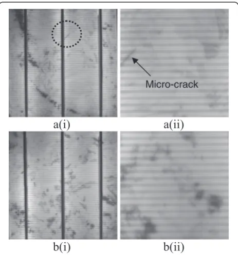
Micro-crack detection in the monocrystalline cell is rela-tively straightforward because this type of cell is character-ized by a uniform background. However, this is not the case for the multicrystalline cell, which contains crystal grains as well as dark areas formed from intrinsic struc-tures like dislocation clusters and grain boundaries. Dis-tinguishing micro-crack pixels from the background (i.e., the multicrystalline grains) is a very challenging procedure because the gray scale values of these two areas are not significantly different. The presence of other defects, such as the dark area, darker grains, and broken fingers, com-plicates the problem. In spite of these difficulties, the iden-tification is still possible because the micro-cracks tend to appear in the form of strong lines with a low intensity and a high gradient. Figure 1a (i) shows an example EL image
of a defected solar cell, and its close-up view of the region containing the micro-crack is displayed in Figure 1a (ii). For comparison, the EL image of a good solar cell is presented in Figure 1b (i), and its close-up view is shown in Figure 1b (ii). Meanwhile, the scan-line profile of gray level and gradient of the solar cell defected with a micro-crack is shown in Figure 2b,c, respectively. These figures highlight the unique textural characteristics of the micro-crack pixels.
All EL images used in this study including those shown in Figure 1 are 8-bit gray scale measuring 1,178 × 1,178 pixels in size. Other examples of defected solar cells containing various types and shapes of micro-cracks are shown in Figure 3. The micro-crack pixels appear in the form of a line or an intersection of lines forming a star-like artifact as depicted in Figure 3a. For comparison, Figure 3b shows examples of good solar cells highlighting the presence of dark regions having arbitrary shapes and sizes. They are formed by an aggregate of dislocation clusters or grainy materials, resembling dark shaped areas when visualized under the EL illumination. As seen from this figure, the presence of many dark areas or regions in both good and defected samples makes a micro-crack inspection an ex-tremely difficult process. However, a close examination of Figure 3a reveals that micro-crack pixels exhibit unique shapes or patterns compared to dark regions even though
a(i)
a(ii)
b(i)
b(ii)
Micro-crack
Figure 1Examples of multicrystalline solar cell images. (a)
they have the same gray scale values. Thus, some form of image analysis is needed in order to facilitate accurate de-tection and efficient classification.
In this study, a series of image processing procedures are performed, capitalizing the unique textural properties and multicrystalline grain inhomogeneity of the solar cell. The details are described in the next section.
2.2 Image pre-processing
As seen in Figures 1 and 3, the EL images of the solar cell contain various features, such as fingers (horizontal lines) that are periodic in nature and perpendicular to the bus-bar (thicker vertical lines in Figure 1a (i) and Figure 1b (i)). A close inspection of these figures revealed that the inten-sity distribution is not uniform both within the cell and among the cells. The presence of the broken fingers and non-uniform background luminescence directly affects the micro-crack analysis, especially if a simple image segmenta-tion technique is used. The solusegmenta-tions to these problems are to remove the periodic interruption of fingers and minimize the effect on background inhomogeneity on image process-ing. This can be done by filtering in the frequency domain.
LetIObe the original EL image of sizem×n, and^IOðu;vÞ
is its Fourier transform representation. Due to the orthog-onal properties, the fingers in the spatial domain appear as a straight vertical line located at the center of a spectrum. This line is dominated by high-frequency components because the contrast between fingers and background is relatively higher compared to other inhomogeneities. Meanwhile, the low-frequency regions contain other important components such as the grain boundaries, dislocation clusters, and micro-cracks. Hence, only the high-frequency components located around the vertical line needs to be removed while retaining the low-frequency components. Therefore, a custom-made filter is constructed to remove these artifacts. The filter function is given below:
^ V uð ;vÞ ¼
0; D u^ð ;vÞ≥d and n
2−w≤D u^ð ;vÞ≤ n 2þw
1− exp −D^
2ðu;vÞ
2σ2
; otherwise 8
> > < > > :
ð1Þ where
^
D uð ;vÞ ¼
ffiffiffiffiffiffiffiffiffiffiffiffiffiffiffiffiffiffiffiffiffiffiffiffiffiffiffiffiffiffiffiffiffiffiffiffiffiffiffiffi u−m
2
2
þ v−n
2
2
r
ð2Þ
(a)
(b)
Figure 3Examples of micro-cracks and dark regions. (a)Solar cells with various types and shapes of micro-cracks.(b)Good samples showing the formation of dark regions.
(a)
50 100 150 200 250
96 128 160
Pixels
Gray
(b)
50 100 150 200 250
0 8 16
Pixels
Gradient
(c)
Micro-crack
Figure 2Characteristics of micro-crack pixels. (a)Close-up view of the region containing the micro-crack.(b)Gray level profile.
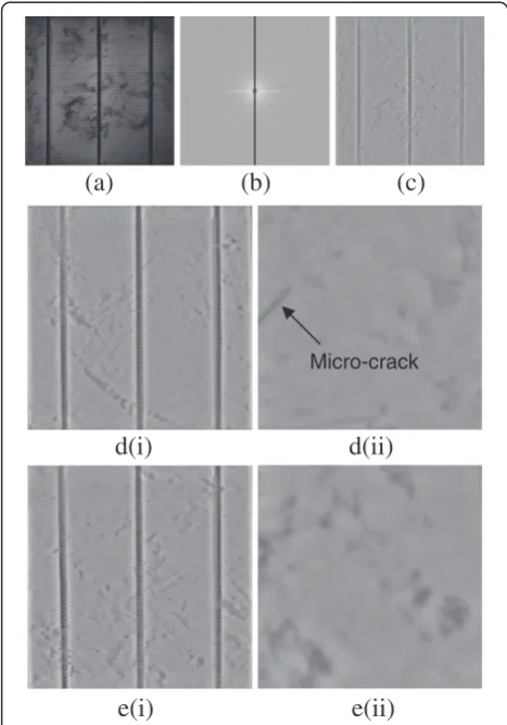
Parameters w, d, and σ in Equation 1 are chosen ex-perimentally. The filtering is performed by pixel-to-pixel multiplication between ^IOðu;vÞ and V u^ð ;vÞ to produce
^
Ieðu;vÞ as shown in Figure 4a. The resulting image is
inverse Fourier transform, yieldingIe(x,y) in spatial space. To minimize the error resulting from the inconsistency of the gray level between cells, Ie(x,y) is normalized to 128. This filtered image is shown in Figure 4c,d,e. It can be seen from these figures that the fingers have been successfully removed and the background inhomogeneity is reduced. Also, the micro-crack pixels are not affected by this filtering operation as evident from Figure 4d (ii). Therefore, this local processing approach preserves the details in the image while attenuating the slow varying components such as the background irregularities.
2.3 Anisotropic diffusion filtering
This subsection presents an implementation of anisotropic diffusion filtering for image enhancement. As can be seen
in Figure 4d (ii), the micro-crack pixels are characterized with low gray scale values but high gradients. The convo-lution of Ie(x,y) with a simple edge detector (e.g., Sobel kernel) will yield high and low gradients at the edges and micro-crack pixels, respectively. Consequently, the result is that the produced image contains two lines, correspond-ing to regions with high and low intensity gradients. This will give rise to the difficulty in the detection leading to many false negatives. We solved this problem by means of the anisotropic diffusion filtering, which produces equal response to any pixels, including the micro-crack areas. In order to achieve this, the diffusion filter is programmed to take into account not only the intensity of the gradient but also the intensity of the gray level of each pixel. The details are explained below.
The anisotropic diffusion filtering can be defined in terms of the diffused imageId(x,y,t) at iterationt[12]. Mathematically,
Idðx;y;tÞ ¼Idðx;y;t−1Þ þ
1 4
X4
i¼1
c ∇Iid ∇Iid; t>0
ð3Þ
where∇is a gradient andcis a diffusion coefficient that is a non-negative function of the magnitude of the gradient of four Laplacian neighbors, i= {1, 2,…, 4}. Letting s= |∇Id|,
then the diffusion coefficient in Equation3is given as
c sð Þ ¼ exp − s
K 2
ð4Þ
or
c sð Þ ¼ 1þ s
K 2
−1
ð5Þ
These diffusion coefficients exhibit a low value at high gradient purposely to preserve the corresponding edges. On the other hand, these coefficients produce high value at low gradient indicating a strong smoothing effect on the pixels involved. Thus, the anisotropic diffusion filter-ing will produce a smoothed image while the important edges are preserved. ParameterKappearing in Equations 4 and 5 is an edge stopping threshold, and it needs to be correctly specified in order to ensure a successful appli-cation of this filtering strategy. If K is too small, then the diffusion process will be terminated earlier, resulting inId(x,y,t) which is approximately equal toId(x,y, 0). In contrast, fixingKtoo large will significantly diffuse the image, resulting in image blurring. Therefore, the choice of the parameterKis important for producing a diffused image that retains the important edges while smoothing the other regions of the image.
(a)
(b)
(c)
d(i)
d(ii)
e(i)
e(ii)
Micro-crack
In this study, a conventional anisotropic diffusion filter-ing technique is modified to produce the opposite effect. In doing so, the smoothing effect will now take place at the strong edges (high gradient) while the region with low gradient are preserved. This is achieved by inverting the original diffusion coefficient yielding
c sð Þ ¼1− 1þ s
K 2
−1
ð6Þ
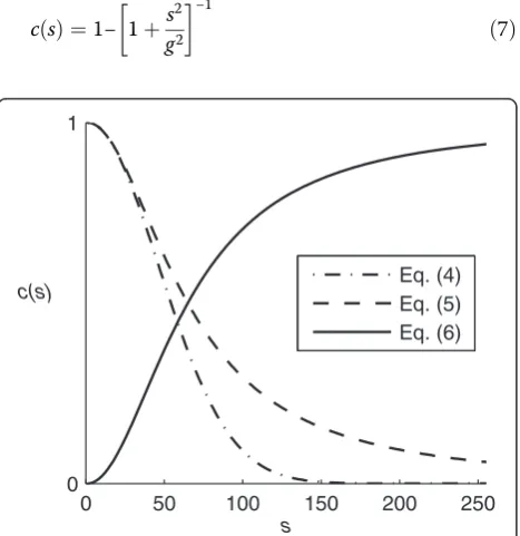
Theoretically, the function in Equation 5 privileges wide regions over smaller ones. Therefore, with modification in Equation 6, this trend is reversed to satisfy the charac-teristics of the micro-crack. Figure 5 shows a response of Equations 4, 5, and 6 with respect to gradient. As shown in this figure, the modified diffusion coefficient increases with the increasing gradient while the responses of the original coefficients are in the opposite sense.
Most of the approach reported in the literature used trial-and-error experiments in determiningK. In contrast, this study used a diffusion coefficient function that elimi-nates the need to use this parameter. Referring to the micro-crack pixels defined in the previous section, we are interested in every pixel with a high gradient but a low intensity value. For this reason, the gradient threshold does not have to be rigidly fixed. In order to achieve this, parameter,Kis replaced with the function that adaptively generates a unique threshold for each pixel using the in-put image gray values. The proposed diffusion coefficient is as follows:
c sð Þ ¼1− 1þs
2
g2
−1
ð7Þ
whereg is a mapping of the image intensity ofId(x,y, 0)
through the sigmoid transfer function given by
g xð ;yÞ ¼ 255
1þ exp½−b Iðdðx;y;0Þ−εÞ
ð8Þ
whereb determines the gradient of ramp in the transfer function andεis a threshold value where the intensity of
Id(x,y, 0) is mapped to the center of the gray scale range.
Equation8is defined as an edge stopping threshold matrix, and it has the same dimension asIe(x,y). Every element in
g(x,y) is the edge stopping threshold value for the corre-sponding pixel inIe(x,y). Equation7is plotted for different
s and g values, and the result is graphically shown in Figure6.
As seen in Figure 6, the response of the diffusion co-efficient varies with the different threshold values. The response is more sensitive when the threshold value is low with respect to the same gradients. High value of the coefficient yields a high diffusivity for the corresponding pixel in the image which leads to blurring effect. As men-tioned earlier, existing techniques only used a single edge stopping threshold value for the whole image. In this study, an adaptive edge stopping threshold function given in Equation 8 is used. This resulted in different threshold values for different pixels depending on their gray scale values through a mapping process.
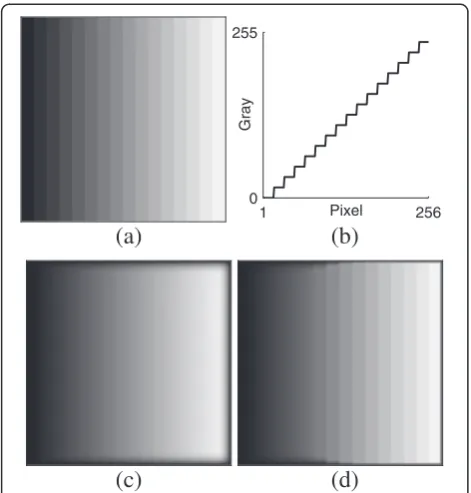
The proposed anisotropic diffusion method described above was tested using a synthetic image of size 256 × 256 pixels. As shown in Figure 7a, this image simulates a gradient profile comprising 16 discrete steps. Figure 7b shows the horizontal line scan of Figure 7a. The dif-fused image using the standard diffusion filter is shown in Figure 7c, while Figure 7d shows the result using the proposed algorithm. Clearly, image processing using stand-ard diffusion filter produced a very blurred image, resulting
0 50 100 150 200 250
0 1
s
c(s) Eq. (4)
Eq. (5) Eq. (6)
Figure 5Diffusion coefficient comparing original and proposed equations.All responses are plotted withK= 64.
56 120
184 248 184
120 56 0 0 1
s g
c(s)
Figure 6Plot of diffusion coefficient with different values of
in incomplete or missing edges. In contrast, the proposed technique affects low gray scale edges only, while the high gray scale edges remain relatively intact. Processing the micro-crack using the proposed technique would result in blurred response in the diffused image since this type of defect is characterized by low gray scale and high gradient. Theoretically, subtracting this image from the original undiffused background would enhance the defect by re-moving some of the background components.
In this study, the proposed anisotropic diffusion filtering is performed in three steps. First, the filtered image,Ie(x,y), is smoothed using a 2-D Gaussian filter of size 5 × 5 yield-ing Id(x,y, 0). Second, the smoothed image is then proc-essed using Equation 8 to produce the edge stopping threshold matrix,g(x,y), which in turn is used to calculate the diffusion coefficient function given by Equation 7. Third, Equation 3 is invoked and the calculation is ter-minated after a few iterations. In this case, the iteration number is determined heuristically and is usually less than 10 in most cases.
The resulting diffused image has a blurred response due to the low-pass filtering effect of the diffusion process. The smoothing effect varies between pixels, and the extent of this depends on the edge stopping threshold value in
g(x,y). For a pixel with a low threshold value, the smooth-ing is significant and yields a very blurred response. In contrast, this image processing technique produces image
which is approximately equal to the original image if the smoothing effect is weak. As previously explained, the resulting image is obtained by subtractingId(x,y,t) from
Id(x,y, 0) to produce the new, enhanced image denoted as IΔ(x,y). Figure 8 illustrates the images produced by these enhancement procedures using Figure 4d (ii) and Figure 4e (ii) as input images. Referring to Figure 8a (iii), the micro-crack line is enhanced and clearly visible after subtraction.
2.4 Post-processing
This section presents a post-processing involved in the segmentation of theIΔ(x,y). It consists of two thresholding stages: (i) binary image reconstruction using double thresh-olding and (ii) the intensity tracing and threshthresh-olding. All threshold values are calculated using an adaptive thresh-olding technique [13]. The general expression of adaptive thresholding is given by
τ¼μ−ασ ð9Þ
whereμ andσare the mean and the standard deviation of the gray level intensity of the input image, respectively, andαis a scaling factor.
In the first stage, we adopted a similar approach based on double thresholding technique described in Nashat et al. [14]. This method requiresIΔ(x,y) to be segmented twice, first using a high threshold value τS and second using a low threshold value τT. Equation 9 is used to compute τS and τT using scaling factors αS and αT, respectively. This segmentation technique produces two binary images referred herein as the seed image BS and the target image BT. In this case BS consists of mainly incomplete but noise-free edges, whereas BT contains complete edges and noise. The next step in the segmen-tation involves reconstructing the final binary imageBF fromBSandBTfollowed by dilation and closing. In this case, BF contains {S1, S2,…, SN} where S represents the shape in the form of binary connected components andN
is the number of shapes following the first stage thresh-olding step. The resulting binary images are presented in Figure 9 using Figure 8a (iii) and Figure 8b (iii) as input images.
Next, the intensity tracing and thresholding are per-formed onBFusingIe(x,y) as the reference image. The purpose of this procedure is to further reduce the noise or the unwanted shapes, such as scratches, dislocation clusters, or grain boundaries. The gray values of these artifacts are relatively higher compared to those of the micro-crack pixels. This procedure helps to improve the feature extraction because it significantly reduces the number of shapes.
For each binary shape S in BF, the value of the gray intensity composed of pixels at the same location and
1 256
0 255
Pixel
Gray
(a)
(b)
(c)
(d)
a(i)
a(ii)
a(iii)
b(i)
b(ii)
b(iii)
Figure 8Image filtering using the proposed anisotropic diffusion technique. (a)Defected sample and(b)good sample: (i) image processing of Id(x,y, 0) using Equation 8 withb= 1 andε¼μIe, (ii)Id(x,y,t) fort= 4, and (iii)IΔ(x,y).
a(i)
a(ii)
a(iii)
b(i)
b(ii)
b(iii)
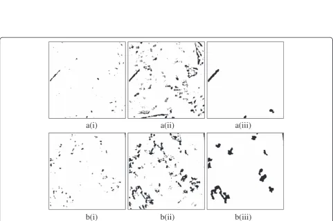
Figure 9Results after image segmentation using double thresholding technique. (a)Defected sample and(b)good sample: (i)BSwith
bounded by the same contourSis traced and extracted from the normalized image after pre-processing. The mean value of the gray intensity for each extracted pixels group is computed. Any shape that has a mean value which is less than the specific threshold is retained in BF. Otherwise, it is treated as noise and hence elimi-nated. Again, the adaptive thresholding given in Equation 9 is used with αtrfixed experimentally while μand σ are obtained fromIe(x,y). These procedures generate a new set of shapes fS1;S2;…;SNFgwhose number is less than
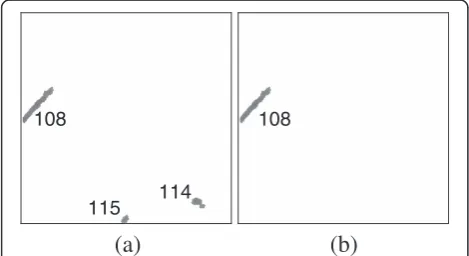
the ones contained in the original set (i.e.,NF≤N). An example of the intensity tracing and thresholding is shown in Figure 10 using Figure 9a (iii) as an input image. In this example, the number of shapes is reduced from 3 to 1.
2.5 Shape analysis
The image processing procedures described in the above paragraph have successfully enhanced micro-cracks as well as other objects while suppressing most of the noise pixels. As seen from previous section, the resulted binary image contains several binary connected components that represent crack and other artifacts. Figure 11 displays some of the objects detected by the algorithm. From this figure, the pixels that represent micro-crack can be distinguished from other artifacts because the former is characterized by some unique shapes and sizes. Therefore, shape analysis is used in order to distinguish between micro-cracks and other objects. This analysis produced features from shape descriptors which are later used in machine learning and classification.
In performing shape analysis, the region-based descrip-tor known as angular radial transform (ART) [15,16] is investigated. The standard number of orders of ART is used to represent all binary shapes. The transform has 36 coefficients, and they are used as shape descriptors. Figure 12 shows examples of the ART spectrum for the micro-crack and arbitrary shapes. As seen in Figure 12,
a normalized ART spectrum for the micro-crack shape has more distinct fluctuation compared to the arbitrary shape. This translated into an increased average distance between the two spectrums and will result to a better dis-crimination of the shapes.
The features extracted are used to train the artificial classifier. In this study, support vector machines (SVMs) are used in machine learning and artificial intelligence. It is a supervised learning algorithm originally developed for two-class classification problems [11]. Therefore, this classifier is suitable for this type of application. Micro-crack shape features are assigned as positive class, while arbitrary shape features are assigned as negative class. Preliminary experiment suggested that the number of micro-crack shapes is far less than that of arbitrary shapes. Due to the unbalanced number of shapes between classes, the SVM classification may result in a bias toward the class having the most number of samples. This problem is addressed by utilizing a soft margin or penalty parameter which was set to different values for each class [17]. This approach is similar to the implementation of a fuzzy membership associated with the penalty parameter [18]. In this case, the optimal values of the penalty parameter for the positive and the negative classes are chosen experi-mentally. Also in this study, the SVM is trained using a kernel based on the Gaussian radial basis function (RBF). In summary, the methods and procedures implemented for micro-crack detection of solar cells are summarized in a block diagram shown in Figure 13.
3. Result and discussion
In this section, the experimental results from the methods and procedures described in the above sections are presented. This includes the image segmentation and classification. All experiments are performed on a desktop computer equipped with a dual core 2.80 GHz processor, 2 GB of RAM, and an installed MATLAB software pack-age. The results obtained in this section are based on 600 samples of which 313 are good samples and the remaining are defected or cracked cells.
3.1 Image processing
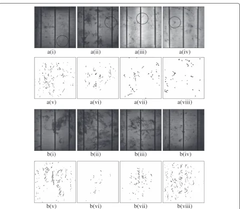
Examples of the segmentation results for defected and good cells are shown in Figure 14. It can be seen from Figure 14a (i-iv) and the corresponding segmented images in Figure 14a (v-viii) that the integrity of the binary connected components (shapes) that represent the micro-crack pixels is well preserved. Referring to these figures, the micro-crack shapes can be easily distinguished from the arbitrary shapes visually. For comparison, the segmentation results of good or intact cells are shown in Figure 14b (v-viii).
For the thoroughness of analysis, the proposed segmen-tation technique is compared with standard methods such
(a)
(b)
108 108
115 114
Figure 10Results from intensity tracing and thresholding. (a)
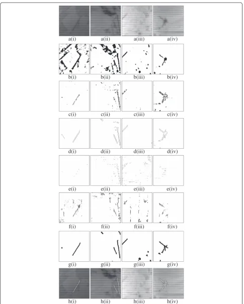
as Otsu's thresholding, the Canny hysteresis, the Sobel edge detector, and the Laplacian of Gaussian (LoG) filter. In addition, a recent method based on Fourier image reconstruction (FIR) [9] is also implemented. Figure 15 shows the close-up view of the results of these different segmentation techniques using images in Figure 14a (i-iv) as input images. In this case, the ground truth images are plotted manually by an expert human inspector. It can be seen from Figure 15b that the segmentation using Otsu's global thresholding technique is able to detect micro-crack as well as other pixels. Meanwhile, both the Sobel detector and Canny hysteresis thresholding resulted in incomplete or disjointed micro-crack pixels. On the other hand, the LoG is only effective in detecting a limited number of micro-crack pixels, particularly the large ones as evident
from Figure 15e. In contrast, the FIR method is accurate when detecting well-defined micro-crack pixels especially the ones appearing like straight lines. This method failed to completely detect star-shaped micro-crack pixels as evident from Figure 15f. In contrast, the results from the proposed segmentation technique are shown in Figure 15g. Clearly, the proposed method is able to detect all shapes and sizes of micro-crack pixels in the image. Close exam-ination of this figures revealed that some unwanted pixels also appeared in the segmented images. They are mostly due to the presence of dark regions in the solar cell. Since their appearance are distinctly different from micro-crack pixels, the use of the ART shape descriptor helped reduce the error resulting from misdetection.
In order to quantitatively evaluate the accuracy of the proposed segmentation technique, the merit based on the
F-measure is used [19]. Mathematically,
F¼2cptcrt
cptþcrt ð10Þ
where cpt and crt are the completeness and correctness indices given by the following equations:
cpt¼ ℓr
ℓGT
ð11Þ
and
crt¼ ℓr
ℓN
ð12Þ
where ℓGT is the number of micro-crack pixels in the
corresponding ground truth image,ℓris the number of
pixels in the segmented image which matches the ground truth micro-crack pixels, andℓNis the total number of
extracted pixels in the segmented image. Examples of ground truth images corresponding to defected cells in Figure15a (i-iv) are shown in Figure15h (i-iv), respectively. On the other hand, the cpt index indicates the com-pleteness of the segmentation technique in detecting
(a)
(b)
Figure 11Results after image segmentation of Figure 3. (a)Micro-crack shapes.(b)Arbitrary shapes.
(a)
(b)
10 20 30 0
1
order ART spectrum
10 20 30 0
1
order ART spectrum
(c)
(d)
EL image
Filtering in the frequency
domain
Gray level normalization
Anisotropic diffusion filter
Image subtraction
Double thresholding Intensity
tracing and thresholding Shape
analysis SVM
Anisotropic diffusion filtering Image pre-processing
Post-processing
Detection result
Figure 13Block diagram of the proposed algorithm.
a(i)
a(ii)
a(iii)
a(iv)
a(v)
a(vi)
a(vii)
a(viii)
b(i)
b(ii)
b(iii)
b(iv)
b(v)
b(vi)
b(vii)
b(viii)
a(i)
a(ii)
a(iii)
a(iv)
b(i)
b(ii)
b(iii)
b(iv)
c(i)
c(ii)
c(iii)
c(iv)
d(i)
d(ii)
d(iii)
d(iv)
e(i)
e(ii)
e(iii)
e(iv)
f(i)
f(ii)
f(iii)
f(iv)
g(i)
g(ii)
g(iii)
g(iv)
h(i)
h(ii)
h(iii)
h(iv)
micro-crack pixels in the defected solar cells. Clearly, from Equation11, cpt is equal to 1 if ℓr=ℓGT, indicating the
perfect match between the number of micro-crack pixels detected by the algorithm and the ground truth image. In contrast, cpt is equal to 0 if there is no match. Meanwhile, the crt index measures the correctness of the segmented image produced. Similarly, this index is equal to 1 if the segmented image matches the ground truth. Practically,
ℓr≤ℓN since micro-crack as well as noise pixels are also
detected. Hence crt also ranges from 0 to 1. Calculating cpt and crt enables theF-measure to be computed using Equation 10. In this case, the higher theF-measure, the better the image segmentation.
The cpt and crt indices calculated from defected cell images in Figure 15 are tabulated in Table 1. These indices are also calculated for the remaining 110 defected cells which are not shown in this paper. The average values are listed in the last column of Table 1. Referring to this table, the completeness of Otsu's method is the highest compared to other algorithms. But this is not the case for correctness as the crt index for this algorithm is the second lowest. Consequently, Otsu's method reconstructs many micro-crack pixels as well as noise as evident visu-ally in the examples in Figure 15. As expected, the Sobel edge detection and Canny hysteresis methods produce only average results for both completeness and correct-ness. The same trend is observed for the FIR method. In contrast, the LoG filter produces the lowest cpt and crt scores, suggesting that this method does not correctly or completely detect micro-crack pixels. Meanwhile, the pro-posed segmentation technique yields the highest crt and the second highest cpt scores. This result suggests that this method has the ability to completely and correctly characterize micro-crack with small amount of noise.
Meanwhile, the results ofF-measure are shown graphic-ally in Figure 16. It can be seen from this figure that the
F-measure score produced by the proposed segmentation algorithm is consistently higher compared to other tech-niques. Overall, the proposed algorithm results inF -meas-ure averaging at 0.0821 compared to 0.0216 FIR, 0.0028 LoG, 0.0258 Canny, 0.02288 Sobel, and 0.0153 Otsu. This again proves that the proposed method is more efficient in detecting micro-cracks in solar cells.
In the anisotropic diffusion filtering technique proposed in this study, there are few parameters that need to be tuned. These parameters areb andεfor the sigmoid map-ping function andtwhich is the number of iterations for anisotropic diffusion. Meanwhile,εcorresponds to the average intensity of the input imageμIe. This simplified the computation of the mapping function as the target micro-crack pixels have the intensity below this average value. Meanwhile, parameterb represents the gradient of the sigmoid mapping function. Higher value of this parameter resulted in steeper gradient for the mapping function. Figure 17 demonstrates the effect of changes in the value of b on IΔ(x,y) using Figure 15a as input images. Clearly from this figure, the best result is obtained forb= 1. Hence, this value was used to process all images reported in this paper.
Another important parameter in the anisotropic diffusion filtering is the number of iterations tin which the image needs to be diffused. This parameter must be properly chosen to ensure successful enhancement of the micro-crack pixels at a minimal computational cost. The higher the number of the iteration, the longer the computational time. Figure 18 shows the normalized values of cpt, crt, and F-measure for the different numbers of iteration. These indices are averaged from 114 defected cells. As can be seen from Figure 18, the highest value ofF-measure occurred att= 1. However, the cpt index corresponding to first iteration is significantly low, indicating the image that it produces is incomplete. Hence, the image needs
Table 1 Completeness and correctness measures of the segmentation results
Measure Method Figure15a (i) Figure15a (ii) Figure15a (iii) Figure15a (iv) Overall average
cpt Otsu 0.9747 0.9706 0.8410 0.6304 0.8832
Sobel 0.2686 0.4029 0.2538 0.4137 0.3703
Canny 0.1248 0.1751 0.0275 0.1048 0.1248
LoG 0.0316 0.0472 0 0.0520 0.0492
FIR 0.4976 0.3668 0.3547 0.2057 0.2952
Proposed 0.9368 0.8873 0.8899 0.7510 0.7185
crt Otsu 0.0026 0.0089 0.0153 0.0586 0.0078
Sobel 0.0064 0.0248 0.0061 0.0123 0.0122
Canny 0.0086 0.0290 0.0015 0.0151 0.0157
LoG 0.0004 0.0016 0 0.0034 0.0014
FIR 0.0156 0.0302 0.0110 0.0286 0.0116
Fig. 15(a)(i) Fig. 15(a)(ii) Fig. 15(a)(iii) Fig. 15(a)(iv) Overall Average 0
0.05 0.1 0.15
Image
F
−Measure
Otsu Sobel Canny LoG FIR Proposed
Figure 16F-measures comparing standard and proposed segmentation techniques.
a(i)
a(ii)
a(iii)
a(iv)
b(i)
b(ii)
b(iii)
b(iv)
c(i)
c(ii)
c(iii)
c(iv)\
d(i)
d(ii)
d(iii)
d(iv)
to be iterated further in order to improve the cpt index. Close examination of Figure 18 revealed that the second highest F-measure occurs at the fourth iteration. Even though the cpt decreases slightly at this iteration, the image is more complete and less noisy compared to the first iteration. A further increase in the number of iteration would result in the decrease of theF-measure as well as the cpt and crt indices. Therefore, the diffusion process of
all images shown in this paper is terminated after the fourth iteration (t= 4).
The performance of the proposed algorithm is also compared with the existing adaptive anisotropic diffusion techniques. Respectively, the images in Figure 19a,b are the results of improved diffusion filters [20,21], while Figure 19c is the image produced by the proposed algorithm. Clearly from this figure, the existing adaptive diffusion
0 5 10 15 20 25 30
0 0.5 1
Iteration,t
Normalized value
cpt crt
F−Measure
Figure 18Average accuracy measures for different numbers of iteration.Images are processed usingε¼μIe andb= 1.
a(i)
a(ii)
a(iii)
a(iv)
b(i)
b(ii)
b(iii)
b(iv)
c(i)
c(ii)
c(iii)
c(iv)
Figure 19Image subtraction results comparing the proposed and existing adaptive anisotropic diffusion filters. (a)Filter proposed in [20] withK0= 2,(b)filter proposed in [21] withK0= 80, and(c)filter proposed in this study. All diffused images used in the subtraction are
filters contain many spurious responses and noisy pixels. Visually, the defect, particularly in Figure 19b, appears to be completely buried in noise, causing the difficulty in extracting features from this image. In contrast, the image produced by the proposed algorithm is less noisy, and the defect can clearly be seen as evident from Figure 19c. Therefore, these results suggest that the existing adaptive anisotropic diffusion filters are not effective in processing micro-crack defects in solar cell images. Moreover, the al-gorithms can be very time-consuming since the diffusion coefficients are computed locally compared to the global technique employed in the proposed method.
3.2 Shape classification
Shape analysis is performed in order to primarily distin-guish between micro-crack and other arbitrary pixels. This is due to the fact that the micro-crack pixels form shapes which are visually distinct like line or star patterns. On the other hand, shapes formed by the spurious intensity variation or gray level discontinuities produce arbitrarily patterns which are also detected by the proposed image processing algorithm. In doing so, the ART shape descrip-tor discussed earlier in Section 2.4 is implemented. The
algorithm is evaluated using 114 defected and 126 intact cells. Altogether, 5,598 shapes have been detected of which 218 belong to the micro-crack category and the remaining are arbitrary patterns. The ART is applied to these shapes, and the results are visualized in principal component plots in Figure 20a. In this case, only the first two dominant components, i.e., first and second components, are used in the visualization.
For comparison purpose, the scattered plots of shape features produced by the well-known methods like (i) the Fourier descriptor (FD) [22], (ii) the generic Fourier descriptor (GFD) [23], and (iii) the projection-based Radon composite features (RCF) [24] are also included in this figure. A close examination of Figure 20 shows that the overlap between micro-crack and other arbitrary shapes is more prominent in Figure 20b,c,d than in Figure 20a. All micro-crack shapes in Figure 20b,c,d occupy the regions that are enclosed within other arbitrary shapes. Clearly, there is no unique demarcation between these two groups in the PCA space. Hence, any attempt to use FD, GFD, or RCF as features in the classification scheme would result in many samples being misclassified. In contrast, the overlap between the groups is less prominent for ART features, as
−10 −5 0 5 10 15
−15 −10 −5 0 5 10 15
1st Principal Component
2nd Principal Component
PCA plot
−10 −5 0 5 10 15
−4 −2 0 2 4
1st Principal Component
2nd Principal Component
PCA plot
−30 −20 −10 0 10
−10 −5 0 5
1st Principal Component
2nd Principal Component
PCA plot
−10 0 10 20 30
−10 −5 0 5 10 15 20
1st Principal Component
2nd Principal Component
PCA plot
(a)
(b)
(c)
(d)
Figure 20Principal component analysis of shape features comparing ART with other standard shape descriptors. (a)ART,(b)FD,(c)
shown in Figure 20a. It can be seen that the other arbitrary shapes are skewed to the right, whereas the micro-crack shapes are skewed to the left. Therefore, it is hypothesized that the features extracted using ART are more separable compared to those extracted using FD, GFD, and RCF.
This hypothesis is validated quantitatively using the sep-arability measure. This measure reflects the discriminative capability in the features of each class; the higher the separability, the higher the discrimination between the groups. Figure 21 shows a comparison of the separability measure between ART, FD, GFD, and RCF. In this case, the separability measure for ART is the highest, registering a value of 12 compared to less than 9 for FD, GFD, and RCF. This result confirms that the features obtained using ART have more discriminative power compared to features obtained using FD, GFD, and RCF.
In this study, altogether 600 randomly selected solar cells have been evaluated from which 240 cells belong to the training set and the remaining 360 cells constitute the test set. Table 2 tabulates the distribution of cells in the training and testing sets. During testing, the classifier produced a positive output when the cell is defected with micro-crack and a negative output when it is intact. For the training set, there are 5,598 shapes, of which 218 belong to micro-crack shapes and the remaining 5,380 are arbitrary patterns. These features are used to train the SVM. For the sake of completeness, the classifi-cations are repeated using a linear discriminant analysis (LDA), quadratic discriminant analysis (QDA), and k -nearest neighbor algorithm (k-NN), from which the results are compared with SVM. Furthermore, the per-formance of each algorithm is quantitatively evaluated in terms of three measurable metrics: (i) sensitivity, (ii) specificity, and (iii) accuracy. These metrics are based on a simple measure of the true positive TP, the true
negative TN, the false positive FP, and the false negative FN. Mathematically, they are defined as follows:
Sensitivity¼ TP
TPþFN ð13Þ
Specificity¼ TN
TNþFP ð14Þ
Accuracy¼ TPþTN
TPþTNþFPþFN ð15Þ
Additionally, the geometric mean is also used in the evaluation. The value of the geometric mean will be high when both the sensitivity and the specificity are high, and the difference between them is small [25]. The use of a geometric mean is an important measure when evaluating the classifier performance, especially for the unbalanced class sizes. The geometric mean is calculated as follows:
G‐Mean¼pffiffiffiffiffiffiffiffiffiffiffiffiffiffiffiffiffiffiffiffiffiffiffiffiffiffiffiffiffiffiffiffiffiffiffiffiffiffiffiffiffiffiffiffiffiffiffiSensitivitySpecificity ð16Þ
The results using the testing set are shown in Table 3. In this table, the SVM is trained with the following parameters: σRBF= 27, C+= 390, and C−= 19. Clearly, from Table 3, the SVM classifier outperformed LDA, QDA, andk-NN in term of sensitivity, accuracy, andG-Mean assessment metrics. Overall, less than 3% of defected cells are misclassified, and more than 80% of good cells are correctly classified. However, thek-NN classifier per-formed best in the classification of good cells with 88% specificity. Nevertheless, the SVM produces the highest
G-Mean, indicating that the error in misclassification of this algorithm is consistently low. Therefore, SVM is overall the best classifier for this type of application.
For completeness, SVM experiments were repeated using FD, GFD, and RCF shape descriptors, and the results
ART FD GFD RCF
0 2 4 6 8 10 12
Shape descriptor
Separability Measure
Figure 21The separability measures comparing the ART, FD, GFD, and RCF shape descriptors.
Table 2 Distribution of intact and defected cells in the dataset
Dataset Defected Intact Total
Training 114 126 240
Testing 173 187 360
Table 3 The classification results of the testing set
Classifier Descriptor Sensitivity Specificity Accuracy G-Mean
LDA ART 0.9306 0.7594 0.8417 0.8406
QDA ART 0.9711 0.7166 0.8389 0.8342
k-NN ART 0.8266 0.8824 0.8556 0.8540
SVM ART 0.9769 0.8021 0.8861 0.8852
FD 0.9711 0.4332 0.6917 0.6486
GFD 0.9595 0.4973 0.7194 0.6908
are also given in Table 3. Clearly, ART outperformed other shape descriptors in all assessment metrics. This again demonstrated that ART gives the best discriminating ability when dealing with this type of shape classification problem compared to other shape descriptors. In addition, the aver-age processing time for each EL imaver-age is approximately 4.1 s which is comparable to the semi-manual inspection by a human expert. Meanwhile, the smallest micro-crack detected by the proposed algorithm is 47 pixels in size which physically corresponds to 6.22 mm in length.
4. Conclusions
The early detection of micro-cracks in solar cells is im-portant in the production of PV modules. In this study, an image processing scheme composed of segmentation procedures based on anisotropic diffusion and shape classi-fication is presented. The results show that the segmenta-tion procedures can detect and identify micro-crack pixels efficiently in the presence of various forms of noise. The anisotropic diffusion filtering with gray level-based diffusion coefficient proposed in this study produced excellent en-hancement and improved segmentation. The advantage of this filtering technique is its ability to enhance the pixels with low gray scale and high gradient such as the micro-crack defects in solar cell. Trained with SVM using 240 samples, this artificial classifier produced a correct classifi-cation rate of consistently higher than 88% with average sensitivity and specificity of 97.7% and 80.2%, respectively. These results are very promising as it demonstrates a first attempt of integrated image processing and ma-chine learning platform toward its eventual application of micro-crack inspection of solar cells.
Competing interests
The authors declare that they have no competing interests.
Acknowledgements
This work is supported by the Malaysia Collaborative Research in Engineering, Science and Technology Centre (CREST) 304/PELECT/6050264/C121.
Received: 23 April 2013 Accepted: 3 March 2014 Published: 21 March 2014
References
1. Solarbuzz, World solar photovoltaic market grew to 27.4 gigawatts in 2011, up 40% y/y. http://www.solarbuzz.com/news/recent-findings/world-solarphotovoltaic-market-grew-274-gigawatts-2011-40-yy-0 (2012). Accessed 27 of January 2013
2. YC Chiou, JZ Liu, YT Liang, Micro crack detection of multi-crystalline silicon solar wafer using machine vision techniques. Sens. Rev.31(2), 154–165 (2011) 3. TK Wen, CC Yin, Crack detection in photovoltaic cells by interferometric
analysis of electronic speckle patterns. Sol. Energy. Mater. Sol. Cells. 98, 216–223 (2012)
4. A Belyaev, O Polupan, W Dallas, S Ostapenko, D Hess, J Wohlgemuth, Crack detection and analyses using resonance ultrasonic vibrations in full-size crystalline silicon wafers. Appl. Phys. Lett.88(11), 111907 (2006) 5. M Demant, S Rein, J Krisch, S Schoenfelder, C Fischer, S Bartsch, R Preu,
Proceedings of the 2011 37th IEEE Photovoltaic Specialists Conference (PVSC) (Seattle, Washington, USA, 2011), pp. 001641–001646
6. M Köntges, I Kunze, S Kajari-Schröder, X Breitenmoser, B Bjørneklett, The risk of power loss in crystalline silicon based photovoltaic modules due to micro-cracks. Sol. Energy. Mater. Sol. Cells.95(4), 1131–1137 (2011) 7. A Bastari, A Bruni, C Cristalli, Proceedings of the, IEEE International
Symposium on Industrial Electronics (ISIE). Bari, Italy2010, 1722–1727 (2010) 8. S Kajari-Schröder, I Kunze, U Eitner, M Köntges, Spatial and orientational
distribution of cracks in crystalline photovoltaic modules generated by mechanical load tests. Sol. Energy. Mater. Sol. Cells.95(11), 3054–3059 (2011) 9. DM Tsai, SC Wu, WC Li, Defect detection of solar cells in
electroluminescence images using Fourier image reconstruction. Sol. Energy. Mater. Sol. Cells.99, 250–262 (2012)
10. DM Tsai, CC Chang, SM Chao, Micro-crack inspection in heterogeneously textured solar wafers using anisotropic diffusion. Image. Vis. Comput. 28(3), 491–501 (2010)
11. C Cortes, V Vapnik, Support-vector networks. Mach. Learn.20(3), 273–297 (1995) 12. P Perona, J Malik, Scale-space and edge detection using anisotropic
diffusion. IEEE. Trans. Pattern. Anal. Mach. Int.12(7), 629–639 (1990) 13. M Sezgin, S Bl, Survey over image thresholding techniques and quantitative
performance evaluation. J. Electr. Imag.13(1), 146–168 (2004)
14. S Nashat, A Abdullah, MZ Abdullah, Unimodal thresholding for Laplacian-based Canny–Deriche filter. Pattern. Recogn. Lett.33(10), 1269–1286 (2012) 15. M Bober, MPEG-7 visual shape descriptors. IEEE. Trans. Circuits. Syst. Video.
Technol.11(6), 716–719 (2001)
16. SK Hwang, WY Kim, Fast and efficient method for computing ART. IEEE. Trans. Image. Process.15(1), 112–117 (2006)
17. K Veropoulos, C Campbell, N Cristianini,Proceedings of the International Joint Conference on AI(Sweden, Stockholm, 1999). pp. 55–60
18. CF Lin, SD Wang, Fuzzy support vector machines. IEEE. Trans. Neural. Net. 13(2), 464–471 (2002)
19. Q Li, Q Zou, D Zhang, Q Mao, SA Fo, F* seed-growing approach for crack-line detection from pavement images. Image. Vis. Comput.29(12), 861–872 (2011) 20. SM Chao, DM Tsai, Astronomical image restoration using an improved
anisotropic diffusion. Pattern. Recogn. Lett.27(5), 335–344 (2006) 21. SM Chao, DM Tsai, An improved anisotropic diffusion model for detail- and
edge-preserving smoothing. Pattern. Recogn. Lett.31(13), 2012–2023 (2010) 22. CT Zahn, RZ Roskies, Fourier descriptors for plane closed curves. IEEE. Trans.
Comput.C-21(3), 269–281 (1972)
23. D Zhang, G Lu, Shape-based image retrieval using generic Fourier descriptor. Signal. Process. Image. Commun.17(10), 825–848 (2002)
24. YW Chen, YQ Chen, Invariant description and retrieval of planar shapes using radon composite features. IEEE. Trans. Signal. Process.56(10), 4762–4771 (2008)
25. M Kubat, RC Holte, S Matwin, Learning when negative examples abound, in Machine Learning: ECML-97, vol. 1224. Lecture Notes in Computer Science, ed. by M Someren, G Widmer, 1224th edn. (Springer, Berlin Heidelberg, 1997), pp. 146–153
doi:10.1186/1687-5281-2014-15
Cite this article as:Anwar and Abdullah:Micro-crack detection of multicrystalline solar cells featuring an improved anisotropic diffusion filter and image segmentation technique.EURASIP Journal on Image and Video
Processing20142014:15.
Submit your manuscript to a
journal and benefi t from:
7Convenient online submission
7Rigorous peer review
7Immediate publication on acceptance
7Open access: articles freely available online
7High visibility within the fi eld
7Retaining the copyright to your article