DOI10.1186/2190-8567-4-4
R E S E A R C H Open Access
Fokker–Planck and Fortet Equation-Based Parameter
Estimation for a Leaky Integrate-and-Fire Model
with Sinusoidal and Stochastic Forcing
Alexandre Iolov·Susanne Ditlevsen· André Longtin
Received: 30 December 2012 / Accepted: 6 June 2013 / Published online: 17 April 2014
© 2014 A. Iolov et al.; licensee Springer. This is an Open Access article distributed under the terms of the Creative Commons Attribution License (http://creativecommons.org/licenses/by/2.0), which permits unrestricted use, distribution, and reproduction in any medium, provided the original work is properly cited.
Abstract Analysis of sinusoidal noisy leaky integrate-and-fire models and compar-ison with experimental data are important to understand the neural code and neural synchronization and rhythms. In this paper, we propose two methods to estimate input parameters using interspike interval data only. One is based on numerical solutions of the Fokker–Planck equation, and the other is based on an integral equation, which is fulfilled by the interspike interval probability density. This generalizes previous methods tailored to stationary data to the case of time-dependent input. The main contribution is a binning method to circumvent the problems of nonstationarity, and an easy-to-implement initializer for the numerical procedures. The methods are com-pared on simulated data.
Keywords First-passage times·Stochastic neuron models·Parameter estimation from stopping times·Fortet integral equation·Fokker–Planck equation
List of Abbreviations
LIF: Leaky integrate-and-fire ISI: Interspike interval
SDE: Stochastic differential equation PDE: Partial differential equation
A. Iolov (
B
)Department of Mathematics and Statistics, University of Ottawa, Ottawa, Canada e-mail:[email protected]
A. Longtin
Department of Physics and Center for Neural Dynamics, University of Ottawa, Ottawa, Canada e-mail:[email protected]
A. Iolov·S. Ditlevsen
Department of Mathematical Sciences, University of Copenhagen, Copenhagen, Denmark S. Ditlevsen
1 Introduction
Information processing in the nervous system is carried out by spike timings in neurons. To study the neural code in such a complicated system, a first step is to understand signal processing and transmission in single neurons. Stochastic leaky integrate-and-fire (LIF) neuronal models are a good compromise between biophys-ical realism and mathematbiophys-ical tractability, and are commonly applied as theoretbiophys-ical tools to study properties of real neuronal systems. A central issue is then to perform statistical inference from experimental data and estimate model parameters. Many electrophysiological experiments on neurons, namely extra-cellular recordings, are only capable of detecting the time of the spike and not the detailed voltage trajec-tory leading up to the spike. Estimating the parameters of the LIF model from this type of data is equivalent to estimating the parameters of a stochastic model from the statistics of the first-passage times only. A common assumption is that the data are well described by a renewal process, thus basing the statistical inference on the interspike intervals (ISIs), assuming these are realizations of independent and identi-cally distributed random variables. Since only partial information about the process is available, the statistical problem becomes more difficult, and no explicit expression for the likelihood is available.
Different methods have been proposed. In the seminal paper [1], a point process approach is proposed. The spike trains of a collection of neurons are represented as counting processes. Time is discretized and the point processes approximated by 0–1 time series. Then the probability of firing in the next time interval is modeled as a function of the spike history. In this way, maximum likelihood estimation is feasible. External stimuli are not considered. In [2], a numerically involved moment method is developed. It uses the first two moments of the first-passage times of the Ornstein– Uhlenbeck process to a constant threshold, which are given as series expressions, and equates them to their empirical counterparts. In [3,4], certain explicit moment re-lations derived from the Laplace transform of the first-passage time distribution are applied, but these are only valid under stimulation (supra-threshold regime). In [5], in-ference is based on numerical inversion of the Laplace transform. In [6], a functional of a three-dimensional Bessel bridge is applied to obtain a maximum likelihood esti-mator. None of these methods are feasible to extend to the time-inhomogeneous case, which is of our interest. In [7,8], an integral equation is used to derive an estimator in the time-homogeneous setting. This approach is readily extended to time varying input, which we will explore in this paper. Some of the above methods are compared in [9]. Finally, a review of estimation methods is provided in [10].
potential dynamics. The estimation problem is solved through numerical solutions to the Fokker–Planck equation, and it is shown that the log-likelihood is concave, thus ensuring a global maximum; see also [20,21]. Because their model is more involved, some approximations to the solution of the Fokker–Planck equation are applied, to ensure acceptable computing times. We will apply the full Fokker–Planck equation to solve our estimation problem, since the computing time is always lower than 2 sec-onds for a sample size of 1000 spikes.
In this paper, we thus describe and discuss two methods to estimate parameters of LIF models with the added complexity of a time-varying input current. We assume that the time-varying current is a sinusoidal wave, but we believe that the approaches generalize to an arbitrary periodic forcing with known frequency. One approach relies on the Fortet integral equation, which is readily extended to the time-inhomogeneous case. An advantage of this approach is that if the transition density of the diffusion in the LIF model is known, as is the case for the Ornstein–Uhlenbeck and the Feller model, the computational burden is limited. A second approach involves numeri-cal solution of the Fokker–Planck equation, where the time-dependence is explic-itly accounted for. After a numerical differentiation, the likelihood function can be calculated providing the maximum likelihood estimator. Nevertheless, we chose an alternative loss function which seems marginally more robust, directly comparing the survival function provided by the solution of the Fokker–Planck equation with its empirical counterpart. The two approaches give similar results and they are more carefully compared in the supplementary online material. Both methods need sensible starting values for the optimization algorithms, and we provide an easy-to-implement initializer. The estimation procedures are compared on simulated data and we find that both algorithms are able to find estimates close to the true values for several different dynamical regimes. We find that for small sample sizes the Fokker–Planck algorithm can be considered marginally preferable, whereas for larger sample sizes the Fortet algorithm becomes marginally superior. Moreover, at high frequencies of the sinusoidal forcing, the Fortet is better at identifying the parameters, though in general there is less information in the data to distinguish between a constant input and the amplitude of the periodic forcing.
2 Model
The time evolution of the voltage of a spiking neuron is modelled by a stochastic process,V, given as solution to the following stochastic differential equation (SDE):
dV (t )=
μ−V (t )
τ +Asin(ωt )
dt+σdW (t ),
t0=0; V (t0)=v0,
tn=inf
t > tn−1:V (t )=vth
forn≥1,
V (tn+)=v0,
Jn=tn−tn−1.
Here,μ is a bias current acting on the cell,τ is the decay time,Aandω are the amplitude and (angular) frequency of the sinusoidal current acting on the cell,σ is the strength of the stochastic fluctuations,W= {Wt}t≥0is a standard Wiener process, andtn+denotes the right limit taken attn. A spike occurs when the membrane voltage
V (t )crosses a voltage threshold, vth, and thenV (t ) is instantaneously reset to the resting potentialv0. The difference between subsequent spike times,Jn=tn−tn−1,
is called the interspike interval (ISI).
We will assume thatτ is known (but see Sect.6for a discussion of the alternative) and nondimensionalize Eq. (1) as follows:
s= t
τ, Xs=
V (t )−v0
vth−v0
, Ws=
W (t )
√
τ , xth=1, α= μτ
vth−v0
, β= σ
√
τ vth−v0
, γ= Aτ vth−v0
, Ω=ωτ
to obtain
dXs=
α−Xs+γsin(Ωs)
ds+βdWs,
s0=0; Xs0=0,
sn=inf{s > sn−1:Xs=xth=1} forn≥1,
Xs+ n =0,
In=sn−sn−1,
(2)
where we have definedIn=Jn/τ. We can also write the dynamics between two spike
timessnandsn+1in terms of elapsed time since the last spike,s=s−sn,s< In+1,
dXs=
α−Xs+γsin
Ωs+φn
ds+βdWs,
s=s−sn,
φn=sn mod 2Ωπ.
(3)
This form of the dynamics highlights that this is not a renewal process since differ-ent trajectories between spikes have differdiffer-ent phase shiftsφn=sn modulo 2π /Ω.
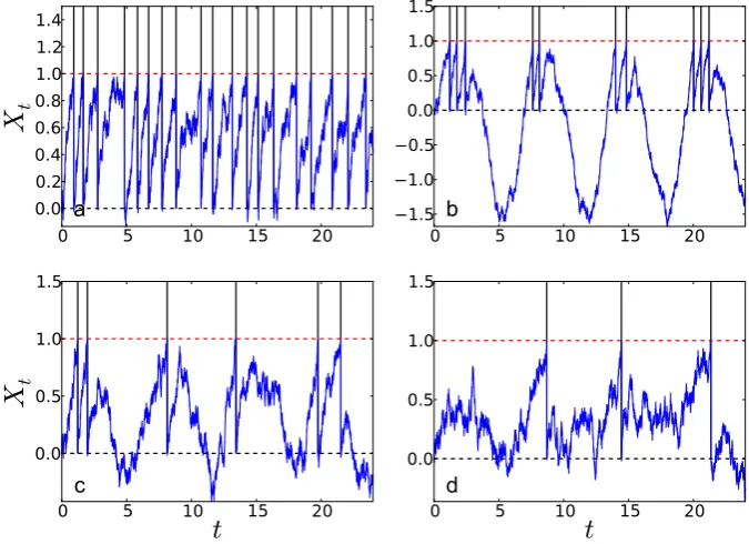
This will be important in the following discussion. The shape of the ISI distribution depends on the model parameters, and it is natural to divide the parameter space in different regimes characterized by their qualitative behavior. Four distinct parameter regimes will be considered; supra-threshold, critical, subthreshold, and supersinu-soidal. To understand the reasoning behind the regime names, observe that in the absence of noise,β=0, the deterministic model will produce spikes if and only if
α+√ γ
1+Ω2>1,
Table 1 Example ofα,β,γ
parameter values for the different regimes, givenΩ=1
Regime name α β γ
Supra-threshold 1.40 0.30 0.14
Supersinusoidal 0.10 0.30 1.98
Critical 0.50 0.30 0.71
Subthreshold 0.40 0.30 0.57
current alone is sufficient for spikes to occur, also in absence of noise, that is,α >1. In the supersinusoidal regime, the sinusoidal current is necessary for spikes to occur in absence of noise, that is,α+γ /√1+Ω2>1 andα≤1. In the critical regime, the sum of the two terms is just barely enough to guarantee deterministic spiking, that is
α+γ /√1+Ω2≈1. Finally, in the subthreshold regime, there would be no spikes without the noise,α+γ /√1+Ω2<1.
Table1tabulates examples of corresponding parameter values for each regime, while Fig.1 shows examples of individual voltage trajectories and their associated spike trains. Figures2 and3 illustrate how each regime behaves for selectedφ’s by plotting the survivor distribution,G¯φ(t ), and the probability density,gφ(t ), both
defined in Eq. (4) below.
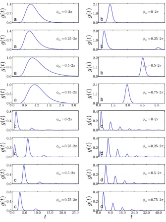
Fig. 2 The four different parameter regimes using the parameter values given in Table1. Illustrated are the probability density functions,gφm(t ), for representativeφm=2π/Ω× {0,0.25,0.5,0.75}. Varying
φmhas, for the most part, the effect of shifting the curves laterally, while varyingα,β,γ changes their characteristic form. For all regimes,Ω=1.asupra-threshold,bsupersinusoidal,ccritical,dsubthreshold
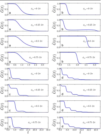
Fig. 3 The four different parameter regimes using the parameter values given in Table1. Illustrated are the survivor distribution functions,G¯φm(t ), for representativeφm=2π/Ω× {0,0.25,0.5,0.75}. Varying
φmhas, for the most part, the effect of shifting the curves laterally, while varyingα,β,γ changes their characteristic form.asupra-threshold,bsupersinusoidal,ccritical,dsubthreshold
2.1 Basic ISI Probability Density Functions
Here, we introduce the notation for the probability density, distribution and survival functions ofIn, an ISI arising from a trajectory produced by Eq. (3),
gφ(τ )dτ :=P
In+1∈ [τ, τ+dτ )|φn=φ
(probability density),
Gφ(t ):=P(In+1≤t|φn=φ)= t
0
gφ(τ )dτ (cumulative distribution),
¯
Gφ(t ):=P(In+1> t|φn=φ)=1−Gφ(t ) (survivor distribution).
(4)
The subscriptφis to stress thatg,G, andG¯ depend on the value ofφnin Eq. (3). This
is the formal statement that in a sinusoidally-driven neuron, the interspike intervals are not identically distributed, and are only independent conditioned on the sinusoidal phase at an interval’s onset. Knowing these distributions would provide the likelihood function, offering estimation by the preferred method of choice, the maximum like-lihood estimator. Unfortunately, explicit expressions for the ISI distribution are not available except for the special case ofγ=0 andα=1; see [3]. Different represen-tations of the likelihood function are available though, see [23], one of which we will use below.
2.2 Fokker–Planck Equation with Absorbing Boundaries
The Fokker–Planck equation is a partial differential equation (PDE) describing the evolution of the probability density, f (x, t ), of Xt. For the sinusoidally-forced
Ornstein–Uhlenbeck process, Eq. (3), with the thresholdxth=1, the PDE is
∂tf(φ)(x, t )= −∂x
α−x+γsinΩ(t+φ)·f(φ)
+∂x2
β2
2 f
(φ)
, x∈(−∞,1). (5)
Due to the reset, we have that at timet=0,Xt=0 and so for the initial conditions
we can write
f(φ)(x, t=0)=δ(x), (6)
whereδ(·)is the Dirac delta function. The spike is represented as a zero boundary condition forf atx=1
f (1, t )=0.
The natural way of using the Fokker–Planck equation in first-hitting-times prob-lems is as follows. Denote the integral off(φ) by F(φ)(x, t )=ξ≤xf(φ)(ξ, t )dξ.
F(φ)(x, t )can be related to the ISI’s survivor distribution function,G¯φ(t ), by
¯
Gφ(t )=F(φ)(1, t ). (7)
Since Eq. (5) has to be solved numerically, we will need to truncate its domain from below. The most natural way to do this, given the dynamics, is to impose reflect-ing boundary conditions at somex=x− (α−γ /√1+Ω2)where the probability mass is very small. For the left (lower) limit of the computational domain, we use the formula
x−=minα−γ /
1+Ω2
mean
−2β/√2
std.dev.
,−0.25.
This choice requires some explanation. In thet→ ∞limit, the distribution of Xt
in Eq. (3) without thresholding is Gaussian with mean given by Eq. (12) (below) and variance equal to β2/2. Thus, to truncate the computational domain for the thresholded process from below, we take the lowest value of the asymptotic mean,
α−γ /√1+Ω2, then from this we subtract two standard deviations, 2β/√2 and set the result to be the lower bound,x−. Finally, if this value forx−happens to be larger than−0.25, we enforce thatx−≤ −0.25.
Numerical considerations lead us to solve forF, instead of f, since delta func-tions are difficult to represent in floating point, while the initial condifunc-tions forF, the Heaviside step function,H (x), faces no such difficulties [24]. The Heaviside step function is defined to be equal to 0 forx <0 and to be equal to 1 forx≥0. At this point, we need to derive the PDE for the distributionF, starting from the PDE for the density,f, Eq. (5).
First, at the lower boundary, it is intuitive that the distribution should be zero,
F (x−, t )=0, whilef (1, t )=0 implies that at the upper boundary∂xF (1, t )=0.
Inside the domain, the PDE itself reformulates as
∂tf (x, t )=∂x
1 2∂x
β2f−α−x+γsinΩ(t−φ)f
so that
∂x∂tF (x, t )=∂x
β2
2 ·∂ 2
xF−
α−x+γsinΩ(t+φ)·∂xF
.
Integrating with respect toxthen gives
∂tF (x, t )=
β2
2 ·∂ 2
xF−
α−x+γsinΩ(t+φ)·∂xF+C(t ),
whereC(t ) is a constant of integration depending on t. Now consider the lower boundary condition,x=x−. Here,F (x−, t )=0 implies that∂tF =0 and so
C(t )= −
β2
2 ·∂ 2
xF −
α−x+γsinΩ(t+φ)·∂xF
. (8)
The right-hand side in Eq. (8) is precisely the reflecting boundary condition onf
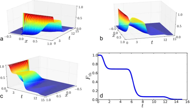
Fig. 4 Example solution to Eq. (9) for(α, β, γ )=(0.5,0.3,0.5√2);Ω=1,φ=π/2. Ina,b,c, we show the full solution in space–timeF (x, t ). Indwe show the time solution at the upper boundary,F (1, t )
Thus, the fully specified PDE forF, which we will be solving frequently in what follows, is
∂tF(φ)(x, t )=
β2
2 ·∂ 2
xF(φ)−
α−x+γsinΩ(t+φ)·∂xF(φ),
⎧ ⎪ ⎨ ⎪ ⎩
F(φ)(x,0)=H (x), F(φ)(x, t )|x=x−≡0,
∂xF(φ)(x, t )|x=1≡0.
(9)
Numerical solutions for Eq. (9) are shown in Fig. 4. We have used the stan-dard Crank–Nicholson finite-difference algorithm (central-differences in space with equally weighted implicit-explicit terms in time, see [25]).
2.3 Fortet Equation
Consider a general form of Eq. (3),
dYt=b(t, Yt)dt+σ (t, Yt)dWt.
Let Φ(y, t|y0, t0):=P[Yt ≤y|Yt0 =y0] be the transition cumulative distribution
ofY. Note that this is the distribution ofYt in absence of a threshold, different from
the distribution given in Eq. (7), which is the distribution of the process constrained to be below the threshold. Now consider an arbitrary time-dependent thresholdvth(t ). The Fortet equation (see [26]) convolves the first-hitting time probabilities,g(t ), with the transition density of the process. Integrating over(−∞, vth(t )), we obtain
1−Φvth(t ), t|v0,0
= t
0
g(τ )1−Φvth(t ), t|vth(τ ), τ
The left-hand side is simply the probability of exceedingvthat timet starting atv0 at time 0. This can also be written as the probability of hittingvthfor the first time at timeτ < t and then exceedingvthat timet starting atvthat timeτ, integrated over allτ.
The Fortet equation is particularly appealing to use when we have an analytical ex-pression forΦ. For the problem at hand,Φis complicated due to the time-dependent forcing. However, the following transformation yields a time-homogeneousY for whichΦ will be tractable, along with an associated moving threshold,vth(t ). This makes feasible the use of the Fortet equation. To obtain this transformation, cf. [27], consider the deterministic version of the SDE in Eq. (3)
dv(t )=α−v+γsinΩ(t+φ)dt,
v(0)=0 (11)
with solution
v(t )=α1−exp(−t )
+√ γ
1+Ω2
sinΩ(t+φ)−ψ−exp(−t )sin(φΩ−ψ );
ψ=arctan(Ω).
(12)
Now takeXt, the solution to Eq. (3) and v(t ), Eq. (12), and letYt=Xt−v(t ).
Then
dYt= −Ytdt+βdW, (13)
which has the time and parameter dependent threshold
vth{α,γ;φ}(t )=vth−v(t ). (14) That is,Xt hits the constant thresholdvthif and only ifYt hits the moving threshold
vth{α,γ;φ}(t ), where the subindex indicates the dependence onα,γ andφ. Therefore,
the ISIs produced byXandY are the same and so are their distributions. Thus,gφ(τ )
satisfies
1−Φ{β}
vth{α,γ;φ}(t ), t|0,0
= t
0
gφ(τ )
1−Φ{β}
vth{α,γ;φ}(t ), t|vth{α,γ;φ}(τ ), τ
dτ, (15)
where
Φ{β}(y, t|y0, t0)=
1
πβ2(1−e−2(t−t0)) y
−∞exp
−(x−y0e−(t−t0))2
β2(1−e−2(t−t0))
dx
3 Parameter Estimation Algorithms
The unknown parameters in Eq. (3) areα,β, andγ, while we assumeΩknown. The reason why the amplitude,γ, is often unknown while the frequency,Ω, is known is that one can usually observe the sinusoidal input and thus its frequency. Further, the encoding of the input into neuronal firing patterns often involves phase locking to the sinusoidal component. However, the actual forcing amplitude at the level of the neuron is usually modified by various synaptic and other filtering processes, unless the cell receives direct sinusoidal current injection.
Our goal is to estimate the structural parameters (α,β,γ) from a sample of spike time data,{i1, . . . , iN}. There are several algorithms for estimating the parameters
for the simpler and more common case ofγ=0. One such algorithm relies on the Fortet equation (see [7,8]), which we extend to the presence of a time-varying cur-rent. A more basic approach is to directly solve the Fokker–Planck equation for the probability density ofXt, [19–21], from which one can derive the survival
distribu-tion ofIn, and use this to compare against the empirical survival distribution of In
obtained from data. An approximate maximum likelihood approach is also possible by numerical differentiation. The relation between Fokker–Planck equations and the first-passage time problem is discussed in most introductory books on stochastic anal-ysis; see, for example, [28]. A recent review of this approach for the simpleγ =0 case in neuronal modeling can be found in [21], wherein the first passage problem is discussed at great lengths in the context of spiking neurons. We will use this in Sect.2.2. A more elaborate approach using the Fokker–Planck equation to approxi-mate the hitting time distribution is given in [29]. The techniques in [29] avoid the need to compute the Fokker–Planck PDE numerically, instead approximating it with analytically known solutions. This approach might offer significant computational savings, but since this would at most amount to a computational speed-up of our algorithm, we have left this unexplored for now.
The immediate problem in generalizing the aforementioned approaches to the case ofγ=0 is that theIn’s are no longer identically distributed since the phaseφn−1of thenth intervalIndepends ontn−1, the time the previous spike occurred. TheIn’s are
also dependent, but conditionally independent givenφn−1. So the trajectories in each
interval are parameterized by the value ofφn−1 at the time of the last spike/reset. We overcome this obstacle by splitting theIn’s in groups, and approximating the
In’s within groups as coming from identically distributed trajectories in a sense to
be specified below. This approximation which solves the challenge of dependent and non-identically distributed ISIs is the primary contribution of this paper.
3.1 φ-Binning
Before we can use Eq. (9) or (15), we need to deal with the fact thatφis not fixed, but instead eachInstarts with a distinctφn. Our approach is to partition the interval
[0,2π/Ω]intoMbins, whereM N, and represent each bin by the midpoint of the bin,φm. Then we approximate theNobservedφn’s by the closestφmand pretend that
any observedInwas not produced by a trajectory of the form in Eq. (3) withφ=φn,
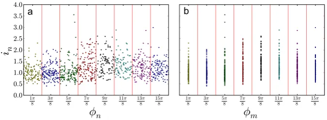
Fig. 5 The raw(in, φn)pairs (a) are binned into a set ofMbins with a representativeφm(b) and the ISIs within each bin are treated as a renewal process. In this illustration,M=8,Ω=1 while the parameters
α,β,γare taken from the supra-threshold regime
error ofφn=φm with having enough data points in each bin in order to obtain a
useful estimate from Eq. (9) or (15).
There is clearly much freedom in how one sets up these bins, but we will do the simplest thing and make them all of equal width,δφ=2π/(ΩM). Eachφnwill
be-long to one and only one of the bins[φm−δφ/2, φm+δφ/2)Mm=1, with center points
φm=δφ/2+(m−1)δφ, form=1, . . . , M. Thus, given an empirically observedIn
with associatedφn, we will pretend that it was produced by the process
dXs=(α−Xs)ds+γsin
Ωs+φm(n)
ds+βdWs,
where
φm(n)=arg min φm
|φn−φm|.
This binning is illustrated in Fig.5.
While we have no rigorous approach to determine the value ofM, our limited experience suggests that givenN=1000 ISIs,M=10, orM=20 gives satisfactory results for very different parameter regimes. In general, choosingM is a balancing act. ForMtoo high, the resulting bins will have too few data points to approximate
¯
G(I )accurately. Therefore,M is forced to be small when sample size is not large. ForMtoo low, the approximation of the phase shifts will be poor, leading to a biased estimate ofG(I )¯ . We illustrate the effect of increasingMin Fig.6. Generally, as long as there are sufficient data points, asM increases, the approximation of using the survival distribution withφminstead ofφnimproves sinceφm(n)→φnasM→ ∞.
In the sequel, we will useM=20 for sample sizes ofN =1000 and M=8 for sample sizes ofN=100.
3.2 Fokker–Planck Algorithm
Within each bin it is clear how to apply Eq. (7). In themth bin, for a givenφm, we
approximateG¯φ(t )by
ˆ¯
Gφm(t )=
#[in> t|φn−1∈ [φm−δφ/2, φm+δφ/2)]
Nm
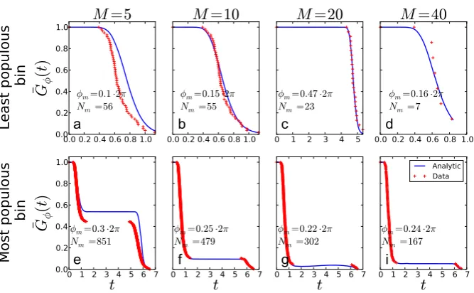
Fig. 6 Effect ofM, the number of bins, on the approximate survival distribution.The full-drawn blue curveis the true survivor distribution given in Eq. (9),the red pointsare the approximation given in Eq. (16). In the figures, the least populous (above) and most populous (below) bin for eachMis shown. The width of the bins isδφ=2π /(ΩM). We have useda,eM=5;b,fM=10;c,gM=20;d,iM=40. AsMincreases, the approximation of using the survival distribution usingφminstead ofφnimproves since
φm(n)→φnasM→ ∞. The data are generated using parameter values from the supersinusoidal regime andN=1000. For this particular data set the largest generated ISI was 6.55 time units
whereNmis the number of ISIs in binm. Using Eq. (7), we define the loss function
L(α, β, γ )=
φm
Nm
sup
t >0
Gˆ¯φm(t )−F
φm
α,β,γ(xth, t ). (17)
The weightNmis included so that bins with larger sample sizes have a larger
influ-ence on the estimates.
To evaluate the supremum in Eq. (17), we spline interpolate the empirically dis-creteGˆ¯ for eachφm, sample at the time nodes of the PDE discretization and finally
take the maximum amongst the sampled values. We then minimizeLusing an opti-mization algorithm (see below, Sect.4) and take our estimatesαˆ,βˆ,γˆto be
ˆ
α,β,ˆ γˆ=arg min
α,β,γ
L(α, β, γ ).
Note that the relation between the spike time survival density,G¯φand the
transi-tion distributransi-tion,Fφ, in Eq. (7) could also allow for an approximate maximum
likeli-hood estimator (MLE), based on maximizing
LMLE(α, β, γ )=
n
loggφn−1(in)
=
n
log−∂tFα,β,γφn−1(xth, t )t=i n,
experience with the MLE approach has been that the quality of the estimates provided are similar to those obtained by minimizing Eq. (17) and that the associated comput-ing times are on the same order. Due to this similarity and in order to keep the paper concise, we include details of the MLE estimates only in the supplementary online material.
3.3 Fortet Algorithm
An alternative approach is to form a loss function from Eq. (15). This is similar to what is done in [7,8] for the simpler case of a constant threshold. Noting that
t
0g(τ )[1−Φ]dτ=E[(1−Φ)1I≤t]where the expectation is taken with respect to the distribution of the random variableI, we can use the fact that the ISIs are ap-proximately independent and invoke the law of large numbers to estimate the integral as
t
0
gφm(τ )
1−Φ{(φ)β}vth{α,γ;φ}(t ), t|vth{α,γ;φ}(τ ), τ
dτ
≈ 1
Nm
in<t
1−Φ{(φ)β}vth{α,γ;φ}(t ), t|vth{α,γ;φ}(in), in
.
We then define the loss function
L(α, β, γ )=
φm Nm sup s>0
1−Φ(φm) {β}
vth{α,γ;φ}(s), s|0,0
− 1
Nm
in<s
1−Φ(φm) {β}
vth{α,γ;φ}(s), s|vth{α,γ;φ}(in), in
ω(φm;α, β, γ )
. (18)
We divide each inner term byω(φm;α, β, γ )=sups>0|1−Φ
(φm)
α,β,γ(vth(s), s|v0)|,
fol-lowing the suggestion in [8]. This scaling ensures that Eq. (15) divided byω(α, β, γ )
will vary between 0 and 1 for all parameter values thus giving sense to the measure defined by the loss function. Since we can solve in closed form forΦ, we have all we need given an observed spike train ofin’s. We evaluate the sup by sampling at
K=500 uniformly spaced points in(0, Imax+]and taking the maximum of the sampled values.
3.4 Initialization of the Algorithms
solving the following PDE:
∂tρ= −U ∂x[ρ] +
β2
2 ∂ 2
x[ρ]. (19)
Its solution given an initial conditionρ(x,0)=δ(x)will be a Gaussian bell moving to the right with speedUand standard deviationσ=β√t.
The survivor functionG(t )¯ can be thought of as the amount of area that has passed the threshold (from the left moving to the right). We can then invert the information aboutG¯ to estimateU andβ. In particular, a Gaussian bell has≈0.158 of its mass more than one standard deviation to the right of its mean. Thus, at timet1such that
¯
G(t1)=0.842, the right tail of more than one standard deviation of the Gaussian bell has crossed the threshold. The threshold is atx=1 and we obtain the following equation:
U t1+β
√
t1=1. (20)
Similarly, at timet2such thatG(t¯ 2)=1−0.842, the Gaussian bell has crossed the threshold except for the left tail and we have
U t2−β
√
t2=1. (21)
If U andβ were constant, then Eqs. (20) and (21) provide two equations in two unknowns. However,U=U (x, t )=(α−x+γsin(Ω(t+φ)))is not constant and we approximateU as
U (x, t )≈α−0.5+γ1 t
t
0
sinΩ(τ+φ)dτ, (22)
i.e., we approximate the space-dependent term,x, with the mid-point between the re-set value,v0=0, and the threshold,vth=1, and we approximate the time-dependent term, sin(Ω(τ+φ)), by its time-average value between 0 andt. If we use the 0th, 1st, and 2nd standard deviation points, we can form 5 equations in 3 unknowns as follows:
αt1+γ s(t1)+2β
√
t1=1+0.5t1,
αt2+γ s(t2)+β
√
t2=1+0.5t2,
αt3+γ s(t3)+0β=1+0.5t3,
αt4+γ s(t4)−1β
√
t4=1+0.5t4,
αt5+γ s(t5)−2β
√
t5=1+0.5t5
current. Indeed, we have found it to be best to use onlyt1andt2. In the following we use only these equations:
αt1+γ s(t1)+2β
√
t1=1+0.5t1,
αt2+γ s(t2)+β
√
t2=1+0.5t2
for the initializer. We can form these equations separately for eachφmbin, thus
result-ing inM×2 equations for the unknownsα,β, andγ. Since we have more equations than unknowns, we use least-squares estimates in a regression to pick out uniqueα,
β, andγ estimates.
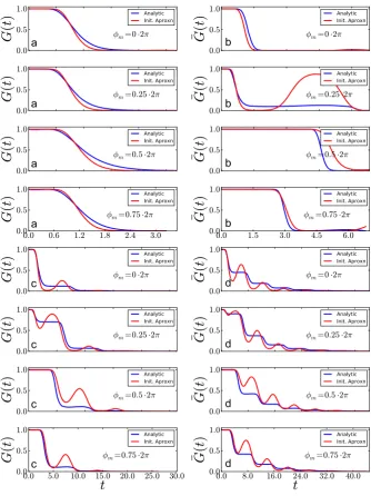
The proposed initialization procedure has two advantages. First, it is automatic, i.e., it requires only the data and no input or guidance from the user. Second, it is extremely fast. While the precise effect of the initializer is shown in Sect.4, it is intu-itively clear that it will work best in the supra-threshold parameter regime when the bell curve is truly moving past the threshold as a whole and less so for subthreshold regimes, when only the diffusive force serves to propel the process to reachvth. The behavior of the initializer in the different regimes is illustrated in Fig.7. What we show in Fig.7is the following: First, we show the survival distribution for a given regime andφmfixed. Then using data generated from such a regime and withφnin
themth bin, the initializer tries to find the best approximation by the motion of a Gaussian bell which will fit these data, in the sense of solving forα,β,γ as previ-ously described. Once this is done, we then show in red the amount of area under this Gaussian bell to the left of the threshold. Of course, the interpretation of the survival distribution for an ISI as a fraction of the area under a moving bell with conserved total area is wrong, but the assumption is useful in automatically generating initial values for the more appropriate approximations to start their work.
4 Method Comparison on Simulated Data
We will now use our algorithms on spike trains simulated from the four different regimes: the supra-threshold, the critical, the supersinusoidal and the subthreshold. We have used 100 sample spike trains per regime, withN =100 as well as N =
1000 spikes per train. In order to perform the numerical minimization of Eqs. (17) and (18), we have used an implementation of the Nelder–Mead algorithm from the SciPy library [30]. The Nelder–Mead algorithm is a non-linear minimization routine which uses a bounding-polygon method to zero-in on the minimum and thus avoids the need to provide the gradient of the loss function. It is the standard non-gradient minimization algorithm.
Fig. 7 The blue curvesare the numerically obtained survivor distributionsG¯φfor the exact parameters in the four regimes (as in Table1) andΩ=1.The red curvesare obtained in the following manner: Simulations using the true parameters were used to generate sample spikes. Using these samples, the initializer algorithm was used to generate estimates forα,β,γ. Using these estimates, the bell curve discussed in Sect.3.4was formed and evolved in time. Thus,the red curvedrawn in the figures measures the area under this bell that is to the left of the threshold at timet.asupra-threshold,bsupersinusoidal,
Fig. 8 Boxplots of parameter estimates for the supra-threshold regime.The upper plots(a,b,c) show estimates usingN=100 sample spikes per estimation, whilethe lower plots(d,e,f) useN=1000.The dashed lineindicates the true parameter value, whilethe red line inside the boxesindicates the median of the estimates.The boxescontain the central 50 % of the estimates.The barsindicate the range of the estimates, except for outliers given bythe points outside the bars, and defined to be more than 1.5 times the interquantile range (the height ofthe box) fromthe box
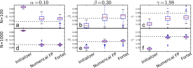
Fig. 9 Boxplots of parameter estimates for the supersinusoidal regime.The upper plots(a,b,c) show estimates usingN=100 sample spikes per estimation, whilethe lower plots(d,e,f) useN=1000.The dashed lineindicates the true parameter value, whilethe red line inside the boxesindicates the median of the estimates.The boxescontain the central 50 % of the estimates.The barsindicate the range of the estimates, except for outliers given bythe points outside the bars, and defined to be more than 1.5 times the interquantile range (the height ofthe box) fromthe box
the supra-threshold, critical and supersinusoidal regimes. The estimators’ variance is especially low in the supra-threshold regime, while it is higher for the critical and supersinusoidal regimes. In the supersinusoidal regime, the two algorithms give ac-curate estimates even though the initializer can be quite off. On the other hand, in the subthreshold regime, the initializer has a performance comparable to that of the two more involved methods. It seems that distinguishing between the constant bias and the sinusoidal current is difficult if their sum is not sufficient to generate spikes without noise.
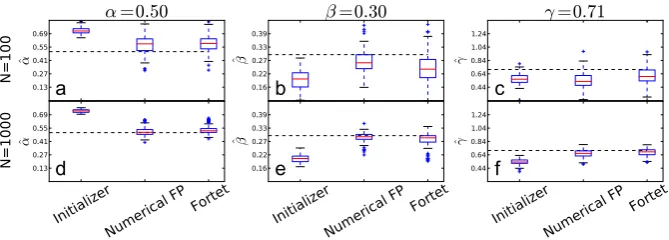
sub-Fig. 10 Boxplots of parameter estimates for the critical regime.The upper plots(a,b,c) show estimates usingN=100 sample spikes per estimation, whilethe lower plots(d,e,f) useN=1000.The dashed line indicates the true parameter value, whilethe red line inside the boxesindicates the median of the estimates. The boxescontain the central 50 % of the estimates.The barsindicate the range of the estimates, except for outliers given bythe points outside the bars, and defined to be more than 1.5 times the interquantile range (the height ofthe box) fromthe box
Fig. 11 Boxplots of parameter estimates for the subthreshold regime.The upper plots(a,b,c) show estimates usingN=100 sample spikes per estimation, whilethe lower plots(d,e,f) useN=1000.The dashed lineindicates the true parameter value, while the red line inside the boxes indicates the median of the estimates.The boxescontain the central 50 % of the estimates.The barsindicate the range of the estimates, except for outliers given bythe points outside the bars, and defined to be more than 1.5 times the interquantile range (the height ofthe box) fromthe box
threshold regime, while the Fortet method has a smaller spread in the supersinusoidal regime. As such, at least in the supersinusoidal regime, the Fortet method seems su-perior. A detailed comparison between the Fortet and the Fokker–Planck estimators for each parameter in each regime can be seen in Fig.12forN=100 and in Fig.13
forN=1000.
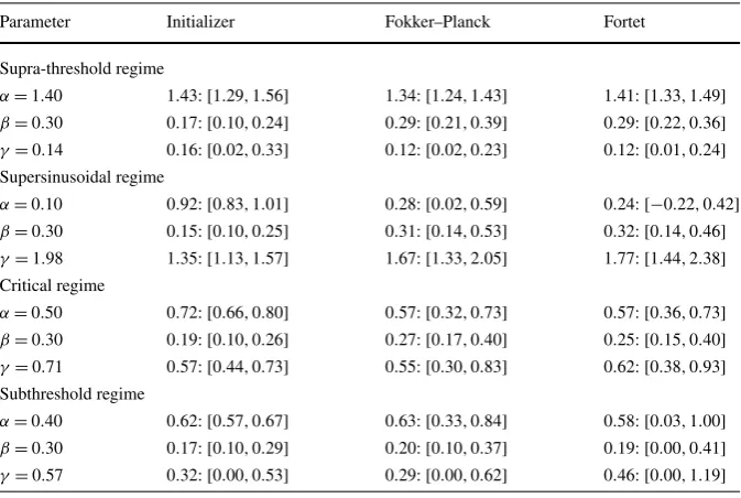
Table 2 Averages and empirical 95 % confidence intervals of the estimates forN=100 spikes per train
Parameter Initializer Fokker–Planck Fortet
Supra-threshold regime
α=1.40 1.43:[1.29,1.56] 1.34:[1.24,1.43] 1.41:[1.33,1.49]
β=0.30 0.17:[0.10,0.24] 0.29:[0.21,0.39] 0.29:[0.22,0.36]
γ=0.14 0.16:[0.02,0.33] 0.12:[0.02,0.23] 0.12:[0.01,0.24] Supersinusoidal regime
α=0.10 0.92:[0.83,1.01] 0.28:[0.02,0.59] 0.24:[−0.22,0.42]
β=0.30 0.15:[0.10,0.25] 0.31:[0.14,0.53] 0.32:[0.14,0.46]
γ=1.98 1.35:[1.13,1.57] 1.67:[1.33,2.05] 1.77:[1.44,2.38] Critical regime
α=0.50 0.72:[0.66,0.80] 0.57:[0.32,0.73] 0.57:[0.36,0.73]
β=0.30 0.19:[0.10,0.26] 0.27:[0.17,0.40] 0.25:[0.15,0.40]
γ=0.71 0.57:[0.44,0.73] 0.55:[0.30,0.83] 0.62:[0.38,0.93] Subthreshold regime
α=0.40 0.62:[0.57,0.67] 0.63:[0.33,0.84] 0.58:[0.03,1.00]
β=0.30 0.17:[0.10,0.29] 0.20:[0.10,0.37] 0.19:[0.00,0.41]
γ=0.57 0.32:[0.00,0.53] 0.29:[0.00,0.62] 0.46:[0.00,1.19]
Table 3 Averages and empirical 95 % confidence intervals of the estimates forN=1000 spikes per train
Parameter Initializer Fokker–Planck Fortet
Supra-threshold regime
α=1.40 1.44:[1.40,1.50] 1.36:[1.33,1.40] 1.40:[1.37,1.42]
β=0.30 0.25:[0.22,0.28] 0.29:[0.26,0.32] 0.30:[0.27,0.32]
γ=0.14 0.14:[0.10,0.19] 0.14:[0.10,0.17] 0.14:[0.10,0.18] Supersinusoidal regime
α=0.10 0.90:[0.85,0.92] 0.11:[0.03,0.29] 0.10:[0.03,0.16]
β=0.30 0.18:[0.14,0.23] 0.30:[0.21,0.34] 0.31:[0.22,0.34]
γ=1.98 1.26:[1.16,1.34] 1.92:[1.49,2.05] 1.96:[1.86,2.07] Critical regime
α=0.50 0.73:[0.70,0.75] 0.51:[0.43,0.63] 0.53:[0.45,0.64]
β=0.30 0.20:[0.17,0.24] 0.29:[0.24,0.32] 0.28:[0.19,0.33]
γ=0.71 0.54:[0.44,0.61] 0.66:[0.52,0.76] 0.67:[0.54,0.77] Subthreshold regime
α=0.40 0.62:[0.55,0.65] 0.57:[0.45,0.66] 0.56:[0.26,0.71]
β=0.30 0.20:[0.17,0.26] 0.22:[0.18,0.29] 0.21:[0.13,0.35]
Fig. 12 Estimates based on samples ofN=100 spikes obtained from the Fokker–Planck algorithm against the Fortet algorithm for the four different parameter regimes, with parameter values given in Table1, fixingΩ=1.Each rowcorresponds to one regime and one set of simulations.Each column corresponds to a parameter, with the specific value indicatedabove each plot.a,b,csupra-threshold;d,e,
Fig. 13 Estimates based on samples ofN=1000 spikes obtained from the Fokker–Planck algorithm against the Fortet algorithm for the four different parameter regimes, with parameter values given in Ta-ble1, fixingΩ=1.Each rowcorresponds to one regime and one set of simulations.Each column cor-responds to a parameter, with the specific value indicatedabove each plot.a,b,csupra-threshold;d,e,f
Table 4 Average times±standard deviations in seconds for the algorithm in various regimes. Left:
N=100 spikes;right:N=1000 spikes
Regime Fortet Fokker–Planck Subthreshold 1.29±0.72 0.52±0.21 Supra-threshold 0.83±0.28 0.18±0.20 Critical 0.94±0.42 0.36±0.16 Supersinusoidal 1.36±0.46 0.43±0.17
Regime Fortet Fokker–Planck Subthreshold 9.68±4.98 1.69±0.91 Supra-threshold 3.90±1.05 0.21±0.06 Critical 10.03±2.88 1.28±0.41 Supersinusoidal 10.13±2.24 1.06±0.33
the forminwhich in turn hasNterms and this forms the bulk of the computing time for the Fortet equation. The Fokker–Planck algorithm, on the other hand, scales less-than-linearly withN, since the dependency onNis in forming the approximation,Gˆ¯
to the survivor function and that is not computationally intensive (solving the PDE is).
5 The Effect ofΩ
So far, we have held Ω constant and equal to 1. We now investigate the effect of varyingΩ on the quality of estimates. To narrow the scope, we focus on increasing
Ωwhile keeping the parameters in the critical regime such thatα+γ /√1+Ω2=1 andα=0.5. This amounts to increasingγ withΩ. We do the estimations for four values of Ω= [1,5,10,20]. Similarly to the previous section, we use 100 sample spike trains per parameter set, with each spike train consisting ofN=1000 ISIs.
We show box plots of the estimates for eachΩ in Fig.14. We then directly com-pare the two algorithms, Fortet vs. Fokker–Planck, in Fig.15. The immediate obser-vation is that the Fokker–Planck algorithm fails to keep up at the higher frequencies and consistently underestimatesγ. The Fortet algorithm does better, but still underes-timatesγ. In general, this underestimation ofγ is accompanied by an overestimation ofα. This is exacerbated at higherΩ. We illustrate the relation between estimates for
αvs.γ in Fig.16, where it is quite clear that an underestimation ofγis proportional to the overestimation ofα.
For completeness, we also include the estimates’ average and empirical 95 % con-fidence intervals in Table5.
6 Discussion and Outlook
We have shown two methods to estimate parameters in Eq. (2) from ISI data. Our methods are based on binning the spikes into bins with representative phase shifts. We have devised a constructive procedure to automatically initialize the methods from the data.
Fig. 14 Boxplots of parameter estimates for varyingΩacross[1,5,10,20]while holdingγ /1+Ω2
constant as to keep the parameters in the critical regime.a–cΩ=1,d–fΩ=5,g–iΩ=10,j–lΩ=20. The boxescontain the central 50 % of the estimates.The barsindicate the range of the estimates, except for outliers given bythe points outside the bars, and defined to be more than 1.5 times the interquantile range (the height ofthe box) fromthe box
sample sizes. Both algorithms find sensible estimates most of the time, although they seem less effective in the subthreshold regime. Their performance can be partially attributed to the ability of the initializer algorithm to supply good guesses for starting the optimization iterations.
The Fokker–Planck equation allows for approximate maximum likelihood estima-tion. We chose an alternative loss function, though, because it marginally appeared more robust, possibly because a numerical derivation step is avoided. This is further investigated by simulations in the supplementary online material. The simulations suggest that the distribution of the maximum likelihood estimates in the supersinu-soidal regime appears bimodal, which is not the case for the alternative loss function, Eq. (17).
We have also made a preliminary exploration of the effect ofΩon the quality of the estimates. Our results show that an increase inΩ makes the parametersαandγ
more difficult to estimate accurately and at highΩ,γ is underestimated, whileαis over-estimated. We find that in this scenario, the Fortet algorithm does a markedly more accurate job then the Fokker–Planck algorithm.
Fig. 15 Estimates based on samples ofN=1000 spikes obtained from the Fokker–Planck algorithm against the Fortet algorithm for a parameter set in the critical regime, while varyingΩacross[1,5,10,20] and holdingγ /1+Ω2andαconstant.a,b,cΩ=1;d,e,fΩ=5;g,h,iΩ=10;j,k,lΩ=20
dramat-Fig. 16 Comparison of αˆ vs.γˆ parameter estimates while varying Ω across[1,5,10,20], holding
γ /1+Ω2constant as to keep the parameters in the critical regime.a,b,cΩ=1;d,e,fΩ=5;g,
h,iΩ=10;j,k,lΩ=20
ically reduced the accuracy in the estimation of the other unknown parameters. The reason is that ifτ is also estimated from a single dataset alongside the other parame-ters, then a reasonable fit can be found to the data for various combinations ofα,β,
Further-Table 5 Averages and empirical 95 % confidence intervals of estimates forN=1000 spikes per train in the critical regime for varyingΩacross[1,5,10,20]. Note that the upper subtable corresponds to the third subtable in Table3; numbers differ slightly due to statistical fluctuations in the simulations
Parameter Initializer Fokker–Planck Fortet
Ω=1
α=0.50 0.73:[0.69,0.75] 0.52:[0.45,0.61] 0.52:[0.44,0.62]
β=0.30 0.20:[0.17,0.25] 0.29:[0.24,0.33] 0.29:[0.22,0.34]
γ=0.71 0.54:[0.44,0.62] 0.64:[0.53,0.75] 0.68:[0.55,0.81]
Ω=5
α=0.50 0.88:[0.76,0.99] 0.78:[0.61,0.89] 0.64:[0.39,0.99]
β=0.30 0.24:[0.17,0.31] 0.26:[0.20,0.34] 0.27:[0.12,0.34]
γ=2.55 0.85:[0.00,1.65] 0.92:[0.00,1.68] 1.86:[0.00,3.10]
Ω=10
α=0.50 0.90:[0.78,0.99] 0.71:[0.52,0.88] 0.58:[0.37,0.86]
β=0.30 0.25:[0.18,0.33] 0.26:[0.20,0.35] 0.28:[0.23,0.32]
γ=5.02 2.82:[0.92,4.38] 2.72:[0.95,3.88] 4.32:[1.20,6.49]
Ω=20
α=0.50 0.93:[0.76,1.02] 0.75:[0.50,0.92] 0.62:[0.31,0.97]
β=0.30 0.27:[0.20,0.33] 0.29:[0.20,0.43] 0.29:[0.25,0.33]
γ=10.01 5.35:[0.00,12.29] 3.98:[0.00,6.83] 7.48:[0.00,13.96]
more, intracellular recordings suggest that a hard threshold is a rough approximation and an exponential voltage-dependent spiking intensity is more realistic [33].
While our work has used a very specific form of the periodic forcing term, namely
γsin(Ωt ), it is clear how to apply the approach to an arbitrary periodic function. This can be done as long as one knows where in the period of oscillation a spike has occurred. If that is the case, then the binning procedure can be applied and the estimation methods proposed can be attempted.
Competing Interests
The authors declare that they have no competing interests.
Authors’ Contributions
All authors contributed equally to the writing of this paper. All authors read and approved the final manuscript.
References
1. Brillinger DR:Maximum likelihood analysis of spike trains of interacting nerve cells.Biol Cybern 1988,59:189-200.
2. Inoue J, Sato S, Ricciardi L:On the parameter estimation for diffusion models of single neuron’s activities.Biol Cybern1995,73:209-221.
3. Ditlevsen S, Lánský P:Estimation of the input parameters in the Ornstein–Uhlenbeck neuronal model.Phys Rev E2005,71:011907.
4. Ditlevsen S, Lánský P:Estimation of the input parameters in the Feller neuronal model.Phys Rev E2006,73:061910.
5. Mullowney P, Iyengar S:Parameter estimation for a leaky integrate-and-fire neuronal model from ISI data.J Comput Neurosci2008,24(2):179-194.
6. Zhang X, You G, Chen T, Feng J:Maximum likelihood decoding of neuronal inputs from an interspike interval distribution.Neural Comput2009,21(11):3079-3105.
7. Ditlevsen S, Ditlevsen O:Parameter estimation from observations of first-passage times of the Ornstein–Uhlenbeck process and the Feller process.Probab Eng Mech2008,23:170-179. 8. Ditlevsen S, Lánský P:Parameters of stochastic diffusion processes estimated from observations
of first-hitting times: application to the leaky integrate-and-fire neuronal model.Phys Rev E 2007,76:041906.
9. Ditlevsen S, Lánský P:Comparison of statistical methods for estimation of the input parameters in the Ornstein–Uhlenbeck neuronal model from first-passage times data. InCollective Dynam-ics: Topics on Competition and Cooperation in the Biosciences. Edited by Ricciardi LM, Buonocore A, Pirozzi E. Melville: Am Inst of Phys; 2008:171-185. [American Institute of Physics Proceedings Series, vol CP1028.]
10. Lánský P, Ditlevsen S:A review of the methods for signal estimation in stochastic diffusion leaky integrate-and-fire neuronal models.Biol Cybern2008,99(4-5):253-262.
11. Braun HA, Wissing H, Schafer K, Hirsch MC:Oscillation and noise determine signal-transduction in shark multimodal sensory cells.Nature1994,367(6460):270-273.
12. Chacron MJ, Longtin A, St-Hilaire M, Maler L:Suprathreshold stochastic firing dynamics with memory in P-type electroreceptors.Phys Rev Lett2000,85(7):1576-1579.
13. Bulsara AR, Elston TC, Doering CR, Lowen SB, Lindenberg K:Cooperative behavior in periodi-cally driven noisy integrate-fire models of neuronal dynamics.Phys Rev E1996,53(4):3958-3969. 14. Burkitt AN:A review of the integrate-and-fire neuron model: II. Inhomogeneous synaptic input
and network properties.Biol Cybern2006,95(2):97-112.
15. Lánský P:Sources of periodical force in noisy integrate-and-fire models of neuronal dynamics. Phys Rev E1997,55(2):2040-2043.
16. Longtin A, Bulsara A, Pierson D, Moss F:Bistability and the dynamics of periodically forced sensory neurons.Biol Cybern1994,70(6):569-578.
17. Sacerdote L, Giraudo MT:Stochastic integrate and fire models: a review on mathematical meth-ods and their applications. InStochastic Biomathematical Models with Applications to Neuronal Modeling. Edited by Bachar M, Batzel J, Ditlevsen S. Berlin: Springer; 2013. [Lecture Notes in Math-ematics, vol 2058.]
18. Shimokawa T, Pakdaman K, Takahata T, Tanabe S, Sato S:A first-passage-time analysis of the periodically forced noisy leaky integrate-and-fire model.Biol Cybern2000,83(4):327-340. 19. Paninski L, Pillow J, Simoncelli E:Maximum likelihood estimation of a stochastic
integrate-and-fire neural encoding model.Neural Comput2004,16(12):2533-2561.
20. Dong Y, Mihalas S, Russell A, Etienne-Cummings R, Niebur E:Estimating parameters of gener-alized integrate-and-fire neurons from the maximum likelihood of spike trains.Neural Comput 2011,23(11):2833-2867.
21. Sirovich L, Knight B:Spiking neurons and the first passage problem.Neural Comput 2011,
23(7):1675-1703.
22. Longtin A:Mechanisms of stochastic phase locking.Chaos, Interdiscip J Nonlinear Sci1995,
1(5):209-215.
23. Alili L, Patie P, Pedersen J:Representations of the first hitting time density of an Ornstein– Uhlenbeck process.Stoch Models2005,21:967-980.
25. Karniadakis GE, Kirby RM:Parallel Scientific Computing in C++ and MPI. Cambridge: Cambridge University Press; 2003.
26. Fortet R:Les fonctions aléatoires du type de Markoff associées à certaines équations linéaires aux dérivées partielles du type parabolique.J Math Pures Appl (9)1943,22:177-243.
27. Shimokawa T, Pakdaman K, Sato S:Time-scale matching in the response of a leaky integrate-and-fire neuron model to periodic stimulus with additive noise.Phys Rev E1999,59(3):3427-3443. 28. Jacobs K:Stochastic Processes for Physicists: Understanding Noisy Systems. Cambridge: Cambridge
University Press; 2010.
29. Lo C, Chung TK:First passage time problem for the Ornstein–Uhlenbeck neuronal model. In 13th International Conference on Neural Information Processing; 2006:324-333.
30. Jones E, Oliphant T, Peterson P, et al:SciPy: open source scientific tools for Python; 2001. 31. Galasi M:GNU Scientific Library Reference Manual. 3rd edition. Godalming: Network Theory Ltd;
2009.
32. Ditlevsen S, Lánský P:Only through perturbation can relaxation times be estimated.Phys Rev E 2012,86(5):050102.