O R I G I N A L R E S E A R C H
Open Access
Beyond red crowns: complex changes in
surface and crown fuels and their
interactions 32 years following mountain
pine beetle epidemics in south-central
Oregon, USA
Travis Woolley
1,2*, David C. Shaw
1, LaWen T. Hollingsworth
3, Michelle C. Agne
4, Stephen Fitzgerald
1,
Andris Eglitis
5and Laurie Kurth
6Abstract
Background:Mountain pine beetle (Dendroctonus ponderosaeHopkins; MPB), a bark beetle native to western North America, has caused vast areas of tree mortality over the last several decades. The majority of this mortality has been in lodgepole pine (Pinus contortaDouglas ex Loudon) forests and has heightened concerns over the potential for extreme fire behavior across large landscapes. Although considerable research has emerged concerning influence of MPB on forest fuels, there has been little work in the climax lodgepole pine forests of south-central Oregon, USA. Specifically, we assessed changes in forest structure and crown and surface fuels across a chronosequence of time since mountain pine beetle (TSB) epidemics in south-central Oregon (1979 to 2008).
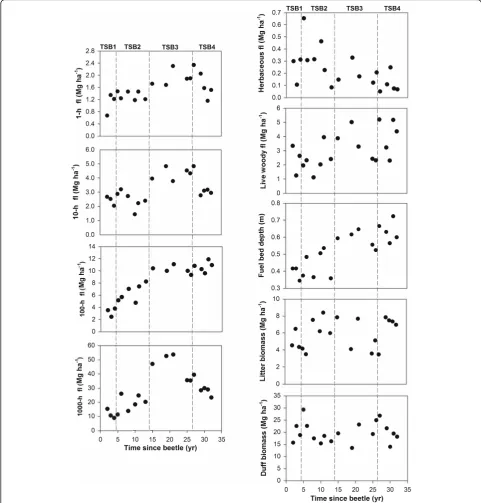
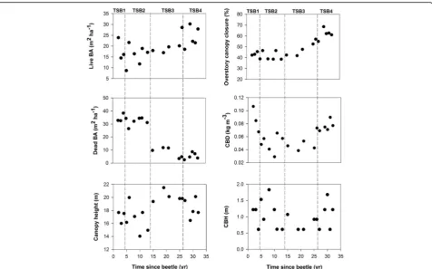
Results: We classified four distinct periods in which significant changes occur in fuels: overstory mortality stage (2 to 4 years TSB), standing snag and snag fall stage (5 to 13 years TSB), regeneration stage (14 to 25 years TSB), and overstory recovery stage (26 to 32 years TSB). Multivariate analyses indicated changes in crown fuels and forest structure following MPB epidemics were driven primarily by basal area of live and standing dead trees, canopy bulk density, canopy base height, and canopy height. Substantial declines in canopy bulk density occurred early (2 to 5 yrs) following beetle activity and slowly recovered over time. The pattern of succession of surface fuels following a MPB epidemic was largely determined by changes over time in 10-h, 100-h, and 1000-h fuel loads, in addition to increasing fuel bed depth. The 100-h fuel load increased over the entire 30-year period, while 1000-h fuel load reached an asymptote 14 to 26 years following epidemic initiation. Live woody fuels increased through the initial overstory mortality stage and began to decrease during the overstory recovery stage.
Conclusions:Our key findings concerning changing fuels and forest structure following a MPB epidemic in south-central Oregon lodgepole pine forests include: 1-h fuels and litter changed little over time, surface fuel loads changed dramatically between the standing snag and the regeneration stages, lodgepole pine remained dominant, and canopy bulk density was low throughout the chronosequence. These factors point to the perpetuation of a lodgepole pine dominated system with a mixed-severity fire regime well into the future.
Keywords:bark beetles,Dendroctonus ponderosae, fuels, lodgepole pine,Pinus contortavar.murrayana
* Correspondence:[email protected]
1
Department of Forest Engineering, Resources, and Management, Oregon State University, 280 Peavy Hall, Corvallis, Oregon 97331, USA
2Present Address: The Nature Conservancy, 114 N. San Francisco Street #205, Flagstaff, Arizona 86001, USA
Full list of author information is available at the end of the article
Resumen
Antecedentes:El escarabajo del pino montaña (Dendroctonus ponderosaeHopkins; MPB), un escarabajo de la corteza nativo del oeste de Norteamérica, ha causado la mortalidad de árboles en vastas áreas durante las últimas décadas. La mayoría de esta mortalidad ha sido en bosques de pino contorta (Pinus contortaDouglas ex Loudon), lo que ha aumentado la preocupación por su potencial de generar incendios de comportamiento extremo a través de grandes paisajes. Aunque muchas investigaciones han surgido concernientes a la influencia de MPB sobre los combustibles forestales, muy pocos trabajos se han realizado en los bosques climáxicos del centro-sur de Oregón, EEUU. Específicamente, determinamos cambios en la estructura del bosque y en los combustibles de la corona y superficiales a través de una crono-secuencia desde la ocurrencia de epidemias de escarabajo del pino de montaña (TSB) en el centro-sur de Oregón (1979 a 2008).
Resultados:Clasificamos cuatro períodos distintos en los cuales ocurrieron cambios significativos en los combustibles: el período de mortalidad del dosel superior (2 a 4 años TSB), el período de muerto en pie y caído (5 a 13 años TSB), el período de regeneración (14 a 25 años TSB), y el período de recuperación del dosel superior (26 a 32 años TSB). Los análisis multivariados indicaron que los cambios en los combustibles de la corona y en la estructura del bosque después de una epidemia de MPB ocurrieron primeramente en el área basal de árboles vivos y muertos en pie, en la densidad de la masa del dosel, en la altura de la base del dosel, y en la altura del dosel. Una sustancial declinación en la densidad de la masa del dosel ocurrió tempranamente (2 a 5 años) después de la actividad del escarabajo y se recuperó lentamente con el tiempo. El patrón de la sucesión de combustibles superficiales después de una epidemia de MPB fue largamente determinado por los cambios en la carga de combustibles de 10, 100, y 1000 horas, en adición a un incremento en la profundidad de la cama de combustible. La carga de los combustibles de 100 h se fue incrementando durante el período de 30 años, mientras que los combustibles de 1000 h alcanzaron una asíntota entre 14 y 26 años después del inicio de la epidemia. Los combustibles vivos leñosos se incrementaron desde la mortalidad inicial del dosel y comenzaron a decrecer durante el período de recuperación del dosel.
Conclusiones: Nuestros descubrimientos clave concernientes a los cambios en los combustibles y en la estructura del bosque luego de una epidemia de MPB en bosques de pino contorta en el centro-sur de Oregón incluyen: a) los combustibles de 1 h y la broza cambiaron muy poco a través del tiempo; b) la carga de combustibles superficiales cambió dramáticamente entre los períodos de muerto en pie y de regeneración; c) el pino contorta permanece como especie dominante; y d) la densidad de la masa del dosel fue baja durante toda la crono-secuencia. De cara al futuro y con un régimen de fuegos de severidad mixta, estos factores apuntan a la perpetuación del sistema dominado por pino contorta.
Background
Bark beetles (Coleoptera: Curculionidae, subfamily
Sco-lytinae), especially mountain pine beetle (Dendroctonus
ponderosae Hopkins; MPB), are important mortality agents in North American coniferous forests (Negron et
al.2008; Raffa et al.2008). Over the past several decades,
MPB has caused mortality on over 30 million ha of
lodgepole pine (Pinus contortaDouglas ex Loudon)
for-ests in the western United States and Canada (Raffa et
al.2008), which has raised concerns about potential for
extreme fire behavior following this widespread
mortal-ity (Page et al. 2014). Fire behavior is driven in part by
forest structure and fuels characteristics; the influence of MPB on forest structure and fuels has become the focus of intense study due to differing hypotheses of potential
effects on fire behavior (Hicke et al. 2012; Jenkins et al.
2014; Perrakis et al. 2014). Mountain pine beetle has
been a cyclical and natural disturbance across lodgepole
pine forested landscapes for as long as records indicate
(Roe and Amman 1970). However, the spatial and
tem-poral scales of recent epidemics are unprecedented over
the last 100 years (Bentz et al. 2009, Raffa et al. 2008,
Brown et al.2010, Edburg et al.2012, Kautz et al.2017).
Previous work in lodgepole pine forests has shown that the influence of MPB epidemics on fuels and forest structure is related to stand density and the proportion of lodgepole pine within a stand at the time of the out-break (influenced by productivity), the proportion of lodgepole pine in larger diameter classes, and time since
previous mortality events (Roe and Amman 1970;
Klutsch et al. 2011; Hicke et al. 2012; Jenkins et al.
2014). The period of elevated MPB activity may last
from a couple of years to a decade in a given stand (Cole
and Amman1980; Hansen2014). During epidemics, up
1980). Throughout many of the lodgepole pine systems previously studied, changes in species composition and structure post outbreak are driven by presence or
ab-sence of non-host species such as subalpine fir (Abies
lasiocarpa [Hook.] Nutt.), mountain hemlock (Tsuga mertensiana [Bong.] Carrière) or Engelmann spruce (Picea engelmannii Parry ex Engelm.) (Collins et al.
2011; Diskin et al. 2011; Kayes and Tinker 2012; Pelz
and Smith2012; Pelz et al.2015).
In general, changes to the structure of crown fuels, surface loadings of fine fuels, and loadings of coarse woody material are the major effects of MPB epidemics
on lodgepole pine forests (Jenkins et al.2014). The
vari-ous phases of structural changes through time have been
previously referred to as “red,” “gray,” and “old” stages
(Edburg et al. 2012; Hicke et al. 2012). The time
neces-sary for a stand to progress through these stages varies
across the species distribution (Jenkins et al.2008; Hicke
et al. 2012). During the red stage, a proportion of the
tree crowns in the canopy have dead and dying foliage. Canopy bulk density drastically decreases through the red stage as dead foliage falls from trees (Simard et al.
2011; Hicke et al. 2012). This stage is relatively
short-lived (2 to 4 yrs) and few other forest structural at-tributes change over this brief time period. Within a few years, the forest enters the gray stage and litter depths, fine fuel loadings, and herbaceous plant and shrub cover
may increase (Page and Jenkins 2007; Collins et al.
2012). Coarse woody debris may also increase in the
gray stage as branches and snags begin to fall (Mitchell
and Preisler 1998; Hicke et al. 2012). The old stage is
characterized by a shift in coarse woody fuel loadings as snags fall, generally 10 to 20 years following MPB attack.
Growth of advanced regeneration may lead to increased canopy bulk density during this stage and decreased can-opy base height. However, depending on stand structure and intensity of MPB-caused mortality, it may take
de-cades for canopy (i.e., canopy closure and canopy bulk
density) to recover to pre-epidemic conditions (Hicke et
al. 2012). The coarse fuel load on the forest floor may
remain high for many decades while growth of shrubs and conifer regeneration create ladder fuels (Page and
Jenkins2007; Jenkins et al.2008; Hicke et al.2012).
In south-central Oregon, Aerial Detection Survey (ADS) data collected since 1980 (USDA Forest Service
2010) indicate the extent MPB-caused lodgepole pine
(Pinus contorta var. murrayana [Greville & Balfour] Engelmann) mortality peaked in 1986 when more than 500 000 ha were detected with varying levels of MPB
ac-tivity (Fig. 1). MPB activity peaked again in 2008, with
over 160 000 ha of affected area detected. Although MPB epidemics are common in this region, research re-garding changes in fuels and forest structure following MPB epidemics has focused on the seral lodgepole pine
forests of the Intermountain West (e.g.,Page and Jenkins
2007; Klutsch et al.2011; Pelz and Smith2012). In
con-trast to most other lodgepole pine forests, thePinus
con-tortavar. murrayana zone of south-central Oregon is a unique setting because lodgepole pine is an edaphic and topoedaphic climax occurring on both well drained and poorly drained pumice soils, associated with broad de-pressions in the landscape where cold air pools (Franklin
and Dyrness1973).
Lodgepole pine forests in this region are often single species, low productivity, largely uneven-aged stands, and are best characterized as having a mixed-severity fire
regime, which may be fuel limited at various stages in
forest development between fires (Geiszler et al. 1980,
Gara et al. 1985, Agee 1993; Heyerdahl et al. 2014). In
contrast, those of the Rocky Mountains, USA, often exist as single-aged stands that are characterized by a stand-replacing fire regime in which climate, rather than
fuels, is limiting (Romme1980; Schoennagel et al.2004).
Historical fire return intervals for the lodgepole pine for-ests of the Fremont-Winema National Forest, Oregon, have been estimated to range between 60 and 350 years
(Stuart 1983). Agee (1981) estimated historical fire
re-turn intervals farther west in Crater Lake National Park, Oregon, at 60 years. Recent research by Heyerdahl et al.
(2014) has corroborated the existence of a
mixed-sever-ity fire regime in dry lodgepole pine on an area of the Deschutes National Forest, Oregon, indicating historical fire return intervals of 26 to 82 years. Lodgepole pine
dwarf mistletoe (Arceuthobium americanum Nutt. ex
Engelm.) is prevalent in the lodgepole forest type in south-central Oregon and has been shown to strongly influence stand structure and fuels following an MPB
epidemic (Agne et al.2014; Shaw and Agne2017). Cone
serotiny is not common in lodgepole pine in
south-central Oregon (Lotan and Critchfield 1990);
therefore, the interaction of fire, bark beetles, and lodge-pole pine seed reproduction may be significantly differ-ent than in areas of the Intermountain West where cone
serotiny frequently occurs (Schoennagel et al.2003). The
lack of cone serotiny helps to define pre-MPB forest structure by providing consistent seed release without a need for fire to initiate regeneration. The lodgepole pine forests of south-central Oregon may be similar to other edaphic climax lodgepole pine forests including: lodge-pole pine forests in the Bighorn Mountains in Wyoming,
USA (Despain 1973); the Wind River Mountains,
Wyo-ming (Reed 1976); as well as those found on obsidian
sands near West Yellowstone, Montana, USA (Pfister et
al.1977). Little is known about the short- and long-term
changes in fuels and forest structure following MPB epi-demic in climax lodgepole pine forests.
To elucidate whether there were novel changes to fuels and forest structure in climax lodgepole pine types in this region compared with other lodgepole pine systems, we addressed the following two questions specifically for the lodgepole pine forests of south-central Oregon: 1) how do fuel profiles (ground, surface, ladder, and crown fuels) change over time in response to MPB epidemics? and 2) what are the key fuels and forest structure com-ponents that drive change over time? In order to recon-struct stand development and resultant ground, surface, ladder, and crown fuels following MPB epidemics and address these questions, we applied a retrospective ap-proach using a space for time (chronosequence) study design.
Methods
Study area
The study area was located in the Pinus contorta zone
(Franklin and Dyrness1973) of central and south-central
Oregon in the Eastern Cascades Slopes and Foothills
ecoregion (Omernik 1987) on the Deschutes and
Fremont-Winema national forests, Oregon, USA (Fig.2).
Stand structure varied from low density, open canopy conditions on drier, less productive sites to closed can-opy conditions composed of larger trees with substantial regeneration on moist, higher productivity sites (Mowat
1960). Overstory tree species were dominated by
lodge-pole pine with other conifer species present in minor
amounts (Fig. 3). Associated tree species also varied by
elevation, and included ponderosa pine (Pinus ponderosa
Lawson & C. Lawson) and white fir (Abies concolor
[Gord. & Glend.] Lindl. ex Hildebr.) at lower elevations, Engelmann spruce in moist cold flats, and subalpine fir,
western white pine (P. monticola Douglas ex D. Don),
and whitebark pine (P. albicaulisEngelm.) at higher
ele-vations. Elevation within the study area ranged from ap-proximately 1450 m to 2500 m and temperatures ranged
from an average daily minimum of−3 °C to an average
daily maximum of 27 °C. Annual precipitation, occurring mainly in the form of snow, ranged from 250 mm in the eastern portion of the study area to 2800 mm at the
highest elevations (PRISM Climate Group2013).
Understory vegetation varied with site productivity, but sites were generally characterized by persistent coarse woody debris; a significant bare ground component; and a mix of sedges, grasses, and shrubs. The most common
shrubs included low-growing antelope bitterbrush (
Pur-shia tridentata [Pursh] DC.), wax currant (Ribes cereum
Douglas), yellow rabbitbrush (Chrysothamnus viscidiflorus
[Hook.] Nutt.), and pinemat manzanita (Arctostaphylos
nevadensis A. Gray). Herbs included Virginia strawberry (Fragaria virginianaDuchesne) and silvery lupine ( Lupi-nus argenteus Pursh). Long-stolon sedge (Carex inops
L.H. Bailey), Ross’sedge (C. rossiiBoott), and grasses such
as western needlegrass (Achnatherum occidentale[Thurb.]
Barkworth) and Idaho fescue (Festuca idahoensisElmer)
were generally common.
Sampling design
We sampled from a 30-year post-MPB-attack chronose-quence (1979 to 2008) in climax lodgepole pine forests of south-central Oregon based on previously developed
plant associations (Hopkins 1979; Volland 1985;
Simp-son 2007) and ADS data, ultimately creating a 2- to
32-year chronosequence of time since beetle (TSB; see
Additional file 1). Although there has been criticism of
chronosequence approaches (Johnson and Miyanishi
2008; Jolly et al.2012), these methods still hold value to
long-term studies are not feasible or data from them are not yet available. Using the local plant association groups, we identified areas of climax lodgepole pine for-ests across three categories of site productivity based on
volume production (low: 0.4 to 0.85 m−3yr−1, moderate:
0.86 to 1.1 m−3yr−1, high:≥1.2 m−3yr−1; Fig.2; Hopkins
1979, Volland1985, Simpson 2007). We then used ADS
(USDA Forest Service 2010) cumulative mortality data
(McConnell et al. 2000) to identify areas that had more
than 12 dead trees ha−1(minimum threshold), which is
considered to be the point at which mortality levels be-come more epidemic in nature (A. Eglitis, Forest Health Protection, USDA Forest Service, Bend, Oregon, USA, unpublished data). Nineteen distinct years of epidemic initiation were identified within the 30 years of ADS data. Using this sampling frame we applied Generalized Random Tessellation Sampling (GRTS) methodology
(Stevens and Olsen2004) in an R statistical software
en-vironment (R Development Core Team 2009) to
ran-domly sample four plot replicates within each
productivity class for a total of 12 plots per epidemic
year (Fig.2), resulting in a 2- to 32-year chronosequence
of time since beetle (TSB).
Field measurements
We sampled trees using an 8.92 m (0.025 ha) radius
cen-tral tree plot. Measurements of individual trees ≥5 cm
diameter at breast height included: DBH (diameter at breast height); tree height; crown class, and crown base height (height to lowest dead or live crown) of live trees and dead standing trees with >50% of needles remaining.
We assigned all snags≥5 cm DBH to a decay class based
on five categories (Thomas 1979). In four 3.2 m radius
subplots, located 25 m from plot center in the ordinal directions, we measured height and basal diameter and recorded species of all tree saplings and seedlings (<5 cm DBH). Within these subplots we also measured shrub cover and several characteristics to determine bio-mass, including basal diameter, height, crown width, and crown volume. A 2 m × 2 m quadrat was nested within each subplot for visual estimation of percent ground
cover (e.g.,downed wood, mineral soil, rock, vegetation)
and percent cover of herbaceous vegetation by species. Surface fuels were measured along 25 m transects in the four cardinal directions using the methods of Brown
et al. (1982). We tallied 1000-h fuels over the entire
length of each transect. For each 1000-h piece, the diam-eter was measured and a decay classes was assigned
based on five categories (Sollins1982). We tallied 100-h
fuels from 15 to 25 m, 10-h fuels from 20 to 25 m, and 1-h fuels from 23 to 25 m along each transect. We mea-sured litter, duff, and surface fuel depths at 10 and 20 m along each transect. A convex densiometer was used to estimate canopy closure at the central tree plot center and each subplot center, following the methods of
Strickler (1959). At the central tree plot center, we
photographed the surface fuels in each cardinal direction (i.e.,along fuels transects), as well as the canopy directly above.
Data analysis
Data preparation
Field-derived counts of 1-h, 10-h, 100-h, and 1000-h
fuels were converted to biomass (Mg ha−1; Harmon and
Sexton 1996, Harmon et al. 2008) using species-specific
density values. We only used 1000 h fuels in decay clas-ses 1 to 3 for further analyclas-ses, omitting the more decomposed decay classes, as extremely decayed mater-ial (decay classes 4 and 5) do not impede resistance to
control efforts (e.g., very difficult for hand crews; Brown
et al. 2003). Seedling, sapling, and shrub counts were
converted to biomass (Mg ha−1) using relationships of
height or basal diameter and mass (Brown 1976; Ross
and Walstad1986; Means et al.1994). Herbaceous cover
estimates were converted to Mg ha−1 using
species-specific equations for the region in BIOPAK
soft-ware (Means et al. 1994). For species with no available
equations, we estimated mass based on equations for similar species. Biomass of duff and litter from depth measurements were calculated using conversion factors
from FIREMON (Lutes et al.2006). We determined can-opy closure for each plot using the average of the five densiometer readings taken in the plot and subplots.
Canopy fuel parameters (canopy base height, canopy bulk density, and canopy height) were calculated using
FuelCalc (Lutes 2014). FuelCalc defines canopy bulk
density as the maximum of the 1.5 m running mean of increments 0.3 m in thickness, while canopy base height is defined as the lowest height at which canopy bulk
density exceeds 0.012 kg m−3(Scott and Reinhardt2001,
Lutes2014). We used a novel approach to calculate
can-opy bulk density using live green trees as well as red (100% of needles remaining, recently attacked) and brown (<100% but >50% of needles remaining, not re-cently attacked) trees to account for changes in the density of foliage as attacked trees died (red) and began to lose their foliage (brown). These coarse estimates of remaining foliage were based on ocular estimates at the time of sampling. FuelCalc uses crown class adjustment
factors to modify canopy fuel load based on trees’
pos-ition in the canopy. Dominant and co-dominant trees with <100% but >50% of needles remaining were reclas-sified as intermediate crown class since the full comple-ment of needles was not present.
TSB stage development
We constructed four post-MPB-epidemic initiation stages based on examining the 75th percentile fuel values (25th percentile for canopy base height) and assessing where natural breaks in the fuel loadings
oc-curred over time (Figs. 4 and 5). We chose to use the
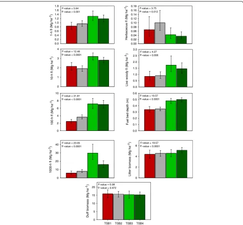
75th percentile for stage development because the upper end of fuel loading distributions is of particular interest and concern to managers due to the perceived connec-tion between fuel load and higher levels of fire intensity, rate of spread, and resistance to control. Several surface and crown fuel parameters influenced the identification of stages. Canopy fuel parameters including canopy bulk density, dead basal area, and overstory canopy closure displayed large changes across the four stages. The sur-face fuels that exhibited substantial change through the stages included live woody, 100-h, and 1000-h fuel loads. Fuel bed depth, herbaceous fuel load, and 10-h fuel load changed to a lesser extent. All other fuels parameters measured were either highly variable or remained stable through all stages. The four stages (TSB1 to TSB4) served as the grouping variable for additional statistical
analyses and are further described in detail in theResults
section.
Statistical analysis
We used the four TSB stages and the fuels data from field plots associated with each stage in a MANOVA fol-lowing the methods outlined by Grice and Iwasaki
(2007) and subsequently applied an ANOVA to make
comparisons of fuel variables that MANOVA indicated were most important. We analyzed the surface and crown fuel strata separately to account for the distinct contributions of crown fuels and surface fuels.
MANOVA We used multivariate analysis of variance
(MANOVA; Grice and Iwasaki 2007) to determine
which fuel and forest structure variables were most in-fluential in changes over time. Given the multivariate na-ture of the fuels complex, a multivariate statistical approach allows greater understanding of which fuels parameters are changing over time while accounting for interacting factors. Surface fuel response variables exam-ined included: 1-h, 10-h, 100-h, and 1000-h fuel loads; litter biomass; duff biomass; fuel bed depth; and herb-aceous and live woody fuel loads (shrub, live seedling, and live sapling). Crown fuel response variables in-cluded: overstory canopy closure, basal area of live trees (live basal area), basal area of standing dead trees (dead basal area), canopy base height, canopy bulk density, and canopy height.
We derived two discriminant functions for each fuel strata. Each function is composed of coefficients that de-scribe the relationship of the dependent fuel variables in that stratum. We then created two simplified multivari-ate composites for each strata. Simplification is the process by which the number of variables in a composite is reduced to those that have the largest effect on the re-sponse variable, thus the final variables included are the most informative and allow for ease of interpretation. Each simplified composite contains only the dependent variables that best discriminate between the stages of the post-MPB-epidemic environment. The final dependent variables were selected based on ranking their coefficient values, whereby larger coefficients (relative to the other coefficients) are retained and those closer to zero were removed. Only two composites were examined for each stratum because their effect sizes warranted their
inclu-sion (Table 1). Effect size can be thought of as the
amount of variance that the composite shares with the response variable. In both the crown and surface fuel strata, the effect size of the second composite was well above zero and, in all cases, nearly half the size of the values for the first composite. In addition, each set of composites had coefficients that differed, providing dif-ferent and complimentary information.
ANOVA We then used these simplified composites
(Grice and Iwasaki 2007) in analysis of variance
(ANOVA) to identify covariates and significant changes in fuels composites over time. Covariates included the proportion of mountain pine beetle mortality (low: 20 to
75 to 200 trees ha−1) derived from ADS data and site productivity (low, moderate, high) derived from plant as-sociation data for climax lodgepole pine in the region. In addition, we performed univariate ANOVAs to obtain estimates of fuel parameters and standard errors for each of the fuel variables that drove the composites. We also performed pairwise comparisons for each of the four
simplified composites between all combinations of TSB stages. We examined both univariate and multivariate assumptions and transformed the following variables to fit assumptions of normality and constant variance: can-opy base height; cancan-opy bulk density (CBD); and herb-aceous, 1-h, 10-h, and 1000-h fuel loads. Bonferroni adjustments were applied, as recommended by Grice
and Iwasaki (2007). Median values were presented for transformed variables. We performed all statistical
ana-lyses using SAS Statistical Software v9.3 (SAS2002).
Results
Fuels and forest structure: time since beetle (TSB) stages
Time since beetle 1 (TSB1): overstory mortality stage (2 to 4 years post-MPB-epidemic initiation)
Often referred to as the red stage, TSB1 is a mix of re-cently killed (red needled), dead (needleless), and living
(green) trees (Fig. 6). The most apparent change that we
noted was in canopy fuels, marked by a nearly 50% de-crease in canopy bulk density during TSB1 due to needle
loss following mortality (Fig.5). Other fuel characteristics
did not demonstrate a consistent trend during this stage. Overall TSB1 can be characterized by a change in canopy fuel characteristics, primarily driven by mortality, needle loss, and consequent changes in canopy bulk density.
Time since beetle 2 (TSB2): standing snag and snag fall stage (5 to 13 years post-MPB-epidemic initiation)
Often referred to as the gray stage, this period of time following MPB initiation was represented by gray stand-ing snags intermixed with the green canopy. A large pro-portion of snag fall (>85% of basal area) occurred by the
end of this stage (approximately 13 years TSB), although some standing snags remained in the regeneration stage (TSB3). The 100-h, 1000-h, and live woody fuel loads
in-creased (Fig. 4), but these trends were not significant
when all years were grouped for TSB2 (Fig. 7). In
addition, overstory canopy closure and canopy bulk
density were lower than in TSB1 (Fig. 8) and continued
to decrease through TSB2 (Fig. 5). This stage can be
characterized by increasing surface fuel loads and con-tinued decrease in canopy fuels.
Time since beetle 3 (TSB3): regeneration stage (14 to 25 years post-MPB-epidemic initiation)
The most notable changes characterizing this stage were continued increases in 10-h, 100-h, and 1000-h fuel
loads, resulting from continued snag fall (Fig. 4). Live
woody fuel loads increased but were highly variable in
this stage (Fig.4), and both live woody fuel load and fuel
bed depth increased compared to TSB2 (Fig. 7) due to
an increase in lodgepole pine seedling and sapling dens-ity. Dead basal area drastically decreased (>90%), as most
snags fell by the end of this stage (Figs.5and8). Overall,
this stage can be characterized by continued increases in surface fuel loads influenced by continued snag fall and initiation and advancement of tree regeneration.
Time since beetle 4 (TSB4): overstory recovery stage (26 to 32 years post-MPB-epidemic initiation)
This stage was represented by an increase in canopy bulk density, overstory canopy closure, and live basal area
com-pared to TSB2 and TSB3 (Fig.8). By 32 years TSB, canopy
bulk density values approached those seen at the
begin-ning of TSB1 (Figs.5and8), while canopy closure
contin-ued to increase and surpass TSB1 (Figs. 5 and 8). The
100-h and live woody fuel loads remained at levels similar
to those of TSB3 (Figs. 4and 7). However, the variability
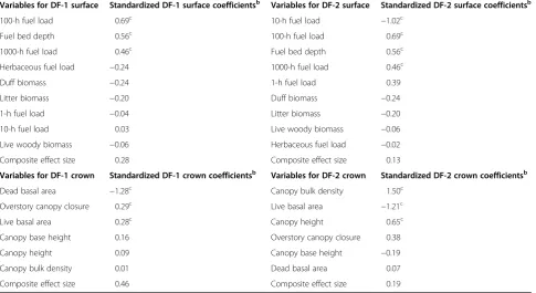
Table 1Discriminant functionacoefficients from MANOVA analysis of surface and crown fuel variables from 2 to 32 years post-MPB
epidemic initiation in lodgepole pine stands of south-central Oregon, USA.aDiscriminant functions are represented as DF-1 surface, DF-2 surface, DF-1 crown, and DF-2 crown.bLarger values indicate stronger relationships.cCoefficient used in simplified multivariate composite to test significance using ANOVA
Variables for DF-1 surface Standardized DF-1 surface coefficientsb Variables for DF-2 surface Standardized DF-2 surface coefficientsb
100-h fuel load 0.69c 10-h fuel load −1.02c
Fuel bed depth 0.56c 100-h fuel load 0.69c
1000-h fuel load 0.46c Fuel bed depth 0.56c
Herbaceous fuel load −0.24 1000-h fuel load 0.46c
Duff biomass −0.24 1-h fuel load 0.39
Litter biomass −0.20 Duff biomass −0.24
1-h fuel load −0.04 Litter biomass −0.20
10-h fuel load 0.03 Live woody biomass −0.06
Live woody biomass −0.06 Herbaceous fuel load −0.02
Composite effect size 0.28 Composite effect size 0.13
Variables for DF-1 crown Standardized DF-1 crown coefficientsb Variables for DF-2 crown Standardized DF-2 crown coefficientsb
Dead basal area −1.28c Canopy bulk density 1.50c
Overstory canopy closure 0.29c Live basal area −1.21c
Live basal area 0.28c Canopy height 0.65c
Canopy base height 0.16 Overstory canopy closure 0.38
Canopy height 0.09 Canopy base height −0.19
Canopy bulk density 0.01 Dead basal area 0.07
Composite effect size 0.46 Composite effect size 0.19
in live woody fuels was quite high in this stage (Fig.4), in-dicating different stand density trajectories within this stage of post-MPB development. Overall, this stage was characterized by a recovery of the overstory (CBD and canopy closure) as saplings and intermediate canopy trees (predominantly lodgepole pine) that survived the MPB epidemic became the new overstory.
Fuels and forest structure: MANOVA
MANOVA illustrated that changes in fuels 2 to 32 years TSB were driven by 3 to 4 fuel variables each for the
sur-face and crown strata (Table 1). Larger values indicate a
stronger relationship in the discriminant function
analyses. Analysis of variance (ANOVA) performed on simplified composites indicated that all four simplified fuels composites (two surface and two crown) were
signifi-cantly different (Bonferroni adjusted α= 0.008) between
stages (Table2). Notably, neither productivity nor level of
mortality were significant covariates for the final
composites.
The first multivariate composite for surface fuels was driven by 100-h fuel load, fuel bed depth, and 1000-h fuel load and could be described as a surrogate for changes in medium to coarse surface fuels and ladder
fuels (Table 1). Pairwise comparisons among all
combi-nations of TSB stages indicated that the simplified
1-h fl (Mg ha -1) 0.0 0.2 0.4 0.6 0.8 1.0 1.2 1.4 1.6 1.8 100-h fl (Mg ha -1) 0 2 4 6 8 10 Litter biomass (M g ha -1) 0 2 4 6 Liv e w oody f l (M g ha -1) 0.0 0.5 1.0 1.5 2.0 2.5 3.0 10-h fl (Mg ha -1) 0 1 2 3 4
TSB1 TSB2 TSB3 TSB4
Duf f biomass (Mg ha -1) 0 5 10 15 20
Fuel bed depth (
m) 0.0 0.1 0.2 0.3 0.4 0.5 0.6 Herbaceous fl (M g ha -1) 0.00 0.02 0.04 0.06 0.08 0.10 0.12 0.14 0.16 0.18 1000-h fl (Mg ha -1) 0 10 20 30 40
F-value = 5.64
P-value = 0.001
F-value = 3.75
P-value = 0.012
F-value = 12.46
P-value < 0.0001
F-value = 31.81
P-value < 0.0001
F-value = 23.05
P-value < 0.0001
F-value = 19.57
P-value < 0.0001 F-value = 19.57
P-value < 0.0001 F-value = 4.27
P-value = 0.006
F-value = 0.08
P-value = 0.972
version of the first composite was significantly different between TSB1 and TSB3, TSB1 and TSB4, and TSB2 and TSB3, but did not show a difference between TSB1
and TSB2 or TSB3 and TSB4 (Table 2). The second
multivariate composite for surface fuels was similar to the first composite, but was strongly driven by 10-h fuel load that increased between TSB2 and TSB3. The 1-h fuel load played a marginal role in driving this pattern, while duff and litter biomass showed a trend of decreas-ing over time. This can be described as a composite representing change in fine to coarse surface fuels and fuel bed depth. However, the simplified version of this composite was only significantly different between TSB2 and TSB3 and did not show a difference between any
other stages using pairwise comparisons (Table2).
Fuels and forest structure: ANOVA
Crown fuel discriminant functions were dominated by dead basal area, live basal area, overstory canopy closure, canopy bulk density, canopy base height, and canopy height. The first multivariate crown fuels composite was driven by dead basal area, overstory canopy closure, and live basal area. This composite can be described as the proportion of live and dead trees and change in tree can-opy closure over time. In pairwise comparison analyses, the simplified version of this composite was significantly
different between all stages except TSB1 and TSB2
(Table2). The second crown fuels composite was driven
by changes in canopy bulk density, live basal area, and canopy height. This composite can be described as a combination of changing canopy bulk density and can-opy height over time. Pairwise comparisons between stages indicated that the simplified version of this com-posite was significantly different between TSB2 and all other stages (TSB1, TSB3, and TSB4), while all other
comparisons were not significant (Table2).
Discussion
Forest fuels structure and composition changes over 32 years following MPB-caused mortality events in south-central Oregon lodgepole pine forests provided in-sights into fire regime characteristics and trajectories into the future compared to other lodgepole pine types.
In contrast to both Simard et al. (2011) and Donato et
al. (2013), who delineated only three post-MPB stages,
our data from south-central Oregon climax lodgepole pine indicated four distinct stages (overstory mortality, standing snag and snag fall, regeneration, overstory re-covery) of fuels changes over 32 years following MPB epidemic. Our key findings concerning changing fuels and forest structure following an MPB epidemic in these lodgepole pine forests include: little change in 1-h fuels
Liv
e BA (
m
2 ha -1) 0 5 10 15 20 25
TSB1 TSB2 TSB3 TSB4
Canopy height ( m) 0 5 10 15 20
TSB1 TSB2 TSB3 TSB4
CBH (m) 0.0 0.5 1.0 1.5 2.0 2.5 CBD (k g m -3) 0.00 0.02 0.04 0.06 0.08 0.10
Dead BA (
m
2 ha -1) 0 10 20 30 40 Overst
ory canopy closure (
%) 0 10 20 30 40 50 60
F-value = 13.88
P-value <0.0001
F-value = 29.15
P-value <0.0001
F-value = 93.21
P-value <0.0001
F-value = 12.13
P-value <0.0001
F-value = 12.43
P-value <0.0001
F-value = 0.62
P-value = 0.6013
and litter over time, dramatic increases in surface fuel loads between TSB2 and TSB3, and continued domin-ance by lodgepole pine. These factors in combination with lower site productivity and low CBD density rela-tive to other regions where lodgepole pine exists points to a perpetuation of a lodgepole pine-dominated system with a mixed-severity fire regime well into the future.
We found no distinction between TSB1 and TSB2 with respect to surface fuels. Slight increases in 100-h fuel load and herbaceous fuel load occurred, but other components of the fine fuel load, such as litter biomass, 1-h, and 10-h fuel loads, did not change between these
stages (Fig. 7). Although this contradicts synthesized
re-sults by Hicke et al. (2012), Agee (1993) notes that litter
is essentially non-existent in this forest type. Perhaps of more consequence, we found that surface fuel loadings changed dramatically between TSB2 and TSB3. Downed
woody debris of all size classes increased (Fig. 7),
con-current with the majority of snagfall (Fig. 8).
Further-more, live woody fuels (representing shrubs and tree seedlings and saplings) also increased between these
stages (Fig. 7) due to low incidence of cone serotiny,
leading to seed dispersal at all phases of stand
development, not just after a fire (Mowat 1960; Lotan
and Critchfield1990). This also indicates that combining
long time spans of TSB into a single structural stage, as
in some previous work (e.g.,Simard et al. 2011), or
omit-ting stands represenomit-ting the range of 15 to 25 years TSB (e.g.,Schoennagel et al. 2012) may miss critical changes in surface fuels following MPB epidemic. While Hicke et
al. (2012) suggest that 100-h and 1000-h fuels slowly
in-crease with time and continue on this trajectory for de-cades, our data support a transition between TSB2 and
TSB3, with little change prior (i.e., between TSB1 and
TSB2) or after (i.e.,between TSB3 and TSB4). As previous
research has discussed (Klutsch et al. 2011), dead fuels,
combined with live intermediate and suppressed lodgepole pine cohort of trees that existed on the site prior to the outbreak, create a dynamic increase in fuels that is main-tained through TSB4 and potentially longer periods of time. These fuels interactions may be extremely important for fire activity during phases when fuels, rather than cli-mate, are the limiting factor for fire activity resulting in a
mixed-severity fire regime (Heyerdahl et al.2014).
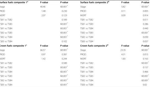
The transition between the initial stage following MPB epidemic initiation (TSB1) and the following stage Table 2Results from ANOVA for simplified composites derived from discriminant function/MANOVA analysis from 2 to 32 years post-MPB epidemic initiation in south-central Oregon, USA. PROD = productivity class; MORT = level of MPB mortality.aSurface fuels composite 1 is composed of the variables: 100-h fuel load, 1000-h fuel load, and fuel bed depthbSurface fuels composite 2 is composed of the variables: 10-h fuel load, 100-h fuel load, 1000-h fuel load, and fuel bed depth*Indicates a statistically significant difference between TSB stages or a statistically significant effect of a covariate (Bonferroni adjustedα= 0.008)cCrown fuels composite 1 is composed of the variables: dead basal area, live basal area, and overstory canopy closuredCrown fuels composite 2 is composed of the variables: live basal area, canopy bulk density, and canopy base height
Surface fuels composite 1a F-value P-value Surface fuels composite 2b F-value P-value
Stage 40.46 ≤0.001* Stage 5.82 ≤0.001*
PROD 1.48 0.230 PROD 0.11 0.895
MORT 2.07 0.129 MORT 0.09 0.914
TSB1 vs TSB2 0.189 TSB1 vs TSB2 0.011
TSB1 vs TSB3 ≤0.001* TSB1 vs TSB3 0.286
TSB1 vs TSB4 ≤0.001* TSB1 vs TSB4 0.440
TSB2 vs TSB3 ≤0.001* TSB2 vs TSB3 ≤0.001*
TSB2 vs TSB4 ≤0.001* TSB2 vs TSB4 0.030
TSB3 vs TSB4 0.102 TSB3 vs TSB4 0.037
Crown fuels composite 1c F-value P-value Crown fuels composite 2d F-value P-value
Stage 66.57 ≤0.001* Stage 23.35 ≤0.001*
PROD 0.97 0.381 PROD 4.31 0.015
MORT 1.42 0.244 MORT 1.83 0.163
TSB1 vs TSB2 0.580 TSB1 vs TSB2 ≤0.001*
TSB1 vs TSB3 ≤0.001* TSB1 vs TSB3 0.157
TSB1 vs TSB4 ≤0.001* TSB1 vs TSB4 0.466
TSB2 vs TSB3 ≤0.001* TSB2 vs TSB3 ≤0.001*
TSB2 vs TSB4 ≤0.001* TSB2 vs TSB4 ≤0.001*
(TSB2) was strongly driven by reduced canopy closure and canopy bulk density. However, the range of canopy bulk density values over the entire chronosequence was low compared to those observed in lodgepole pine for-ests in other regions. For example, in TSB1, mean
can-opy bulk density was approximately 0.07 kg m−3(Fig.8),
while canopy bulk density in lodgepole pine stands in Idaho and Utah, USA, in this same stage ranged from
0.15 to 0.22 kg m −3 (Page and Jenkins 2007). We
hy-pothesized that lodgepole pine forests in our study area
experience mixed-severity fire regime (Agee 1993;
Hey-erdahl et al.2014) in part because canopy bulk density is
low and less likely to support active crown fire. Canopy bulk density continued to decline through TSB2 and
TSB3, with some recovery during TSB4 (Figs. 5 and 8).
Although this general pattern follows the conceptual
framework outlined by Hicke et al. (2012), other
chrono-sequence investigations of MPB and fuels succession have not indicated a significant recovery in canopy bulk density over time following the red stage (Simard et al.
2011; Schoennagel et al. 2012). However, the methods
we used to calculate CBD differed from Simard et al.
(2011), which makes comparisons difficult. Jolly et al.
(2012) pointed out that the categorical reductions to
crown biomass, which subsequently reduced their calcu-lated CBD values, may have been inaccurately applied. Similar to the pattern we detected, but less pronounced,
Schoennagel et al. (2012) reported increasing canopy
bulk density by approximately 30 years post-MPB epi-demic at sites in Colorado and Wyoming, USA. It is likely that the increase in canopy bulk density and can-opy closure shown in our chronosequence will continue and approach or exceed pre-epidemic levels until self-thinning (via suppression mortality or endemic MPB mortality) or low- or moderate-intensity surface fire re-duces tree density.
Most snags fall within 20 years TSB, as noted in other
studies (Mitchell and Preisler 1998); therefore,
signifi-cant increases in 1000-h fuels beyond this point are un-likely. However, we hypothesize that the decrease
observed in 1000-h fuel load in TSB4 (Figs.4and7) was
an artifact of the chronosequence sampling method that we used, not using decay class 4 and 5 in our analysis, and large variations of coarse fuels due to MPB mortal-ity, rather than different rates of decomposition. Previ-ous work in our study area indicates that coarse wood remained relatively sound (decay classes 1 to 3) up to
27 years after snags had fallen (Busse 1994). If most
snags fell between 10 and 20 years TSB, as indicated by
our data (Fig. 4: 1000-h fuel load), we should not see
transition into less sound coarse wood (decay classes 4 and 5) until 37 to 47 years following MPB initiation,
based on decay rates described by Busse (1994). It is
therefore unlikely that there was substantial
decomposition of 1000-h fuels within the time since bee-tle covered by our chronosequence.
This climax lodgepole pine system is influenced by
interacting disturbance agents (Kane et al. 2017), low
site productivity, and dominance by a single tree species,
manifesting in a mixed-severity fire regime (Agee1993),
as compared with the high-severity fire regimes of
lodge-pole pine forests in the Rocky Mountains (Romme1980)
where most previous research on MPB and fuels has been conducted. While fuels are unlikely to contribute substantially to fire activity under most circumstances in Rocky Mountain lodgepole pine forests, in which fire is
primarily limited by climate (Schoennagel et al. 2004),
changes in fuel loadings may have more of an influence on fire in south-central Oregon, where fire may be
lim-ited by fuels or climate at various times (Agee 1993,
Heyerdahl et al.2014). In addition to the low
productiv-ity and mixed-severproductiv-ity fire regime found in this lodge-pole pine system, a major difference contrasting with those found in much of the Rocky Mountain region is that here lodgepole pine is a climax species, and spruce (Picea), fir (Abies), and other pine species do not be-come major components of the tree species composition following MPB epidemics. Our study supported this, and lodgepole pine remained the dominant tree species on the landscape throughout the chronosequence following
the MPB epidemic (Fig. 3). This indicates that these
lodgepole pine systems will maintain similar communi-ties (resilience) following subsequent fire that seems
likely to remain mixed in severity (i.e.,maintained
inten-sity; Kane et al. 2017). When MPB selectively removes
the dominant and co-dominant lodgepole pine from sites in the Rocky Mountain region, changes in compos-ition and stand succession may be accelerated by
releas-ing spruce and fir regeneration (Collins et al. 2011;
Diskin et al. 2011; Kayes and Tinker 2012; Pelz and
Smith 2012; Pelz et al. 2015). However, in the climax
lodgepole pine system of south-central Oregon, the post-MPB succession is facilitated by existing cohorts of lodgepole pine, indicating a resilient ecosystem response
to interacting disturbances (Kane et al. 2017). Although
the difference among regions in the change in species composition over time likely has a minimal effect on fuels over the time covered by the chronosequence in this study, these compositional differences are likely to have considerable effects on the ecology of the forest over longer time scales. The effects of intermittent MPB-caused mortality, multiple interacting disturbance factors, and other unique characteristics of climax
lodge-pole pine communities (e.g., low productivity, lack of
Conclusion
The findings of this study have important implications for several different management objectives. Our results inform fire and forest managers in the region by describing how
fuels change with time following dominant and
co-dominant cohort mortality caused by MPB in these multi-aged, single-species stands. Late TSB2 and TSB3 are likely the most difficult and dangerous settings in which to perform fire suppression activities as snagfall is active and coarse woody debris slows the pace of fire-line construction
(Page et al.2013). Using data from this study in conjunction
with ADS data to map fuels for TSB stages may inform planning prior to fire season in conjunction with existing land management plans and provide the opportunity to manage fires in these areas to achieve resource benefits and
reduce firefighters’exposure to hazard.
Ecologically focused management decisions may be heavily influenced by an MPB epidemic due to known
influences of MPB on biodiversity (Koch et al. 2011;
Treu et al.2014), hydrology (Rex et al.2013; Bradford et
al. 2014), and carbon sequestration (Brown et al. 2010;
Bright et al. 2012; Kasischke et al. 2013). In the
lodge-pole pine forests of south-central Oregon, the impacts may be more nuanced as there is typically no shift in tree species composition following MPB. However, the influence on fuels and forest structure may have implica-tions for fire activity under moderate climate condiimplica-tions, given the mixed-severity fire regime that characterizes this forest type. Using the data and results of this study, forest and fire managers in south-central Oregon can better understand future trajectories of forest structure
and fuels conditions over key time periods (e.g.,TSB2 to
TSB3) in areas affected by mountain pine beetle and therefore better determine the potential effects and risks to multiple resource values.
Additional file
Additional file 1:Figure S1.Photographs depicting examples of fuels
conditions over time following MPB epidemics in south-central Oregon, USA. (PDF 843 kb)
Acknowledgements
We would like to thank the various managers on the Deschutes and Fremont-Winema national forests for supporting this work and their active collaboration and feedback on our work. We would also like to thank M. Huso for statistical advice in sampling design and A. Muldoon for statistical advice in multivariate analyses. This work would also have not been possible without extremely dedicated field crews.
Funding
We acknowledge funding from the Joint Fire Science Program under Project JFSP 09–1–06-17.
Availability of data and materials
The datasets generated or analyzed during the current study are available in the USDA Forest Service Data Archive,https://www.fs.usda.gov/rds/archive/ Product/RDS-2014-0017.
Authors’contributions
TW developed study and sampling design and field data collection protocols, lead data collection, and developed and performed statistical data analysis, and lead drafting and revisions of the manuscript. DCS participated in discussions of study design and field data collection protocols, and assisted in drafting and revisions of the manuscript. LTH provided expertise in fuels data processing and assisted in drafting and revisions of the manuscript. MCA assisted in data collection, analysis, and in drafting and revisions of the manuscript. SF assisted in development of field data protocols, participated in discussions of study design, and assisted in drafting and revisions of the manuscript. AE provided expertise in mountain pine beetle ecology and use of aerial detection survey data in sampling design and data analysis, and assisted in drafting and revisions of the manuscript. LK assisted in development of field data collection protocols, and assisted in drafting and revisions of the manuscript. All authors read and approved the final manuscript.
Ethics approval and consent to participate Not applicable
Consent for publication Not applicable
Competing interests
The authors declare that they have no competing interests.
Publisher’s Note
Springer Nature remains neutral with regard to jurisdictional claims in published maps and institutional affiliations.
Author details
1Department of Forest Engineering, Resources, and Management, Oregon State University, 280 Peavy Hall, Corvallis, Oregon 97331, USA.2Present Address: The Nature Conservancy, 114 N. San Francisco Street #205, Flagstaff, Arizona 86001, USA.3USDA Forest Service, Rocky Mountain Research Station, 5775 US Highway 10 W, Missoula, Montana 59808, USA.4School of Environmental and Forest Sciences, University of Washington, 4000 15th Avenue NE, Seattle, Washington 98195, USA.5USDA Forest Service, Forest Health Protection, 63095 Deschutes Market Road, Bend, Oregon 97701, USA. 6USDA Forest Service, Fire and Aviation Management, 1400 Independence Avenue SW, Washington, D.C. 20250, USA.
Received: 14 September 2018 Accepted: 19 September 2018
References
Agee, J.K. 1981.Initial effects of prescribed fire in a climax Pinus contorta forest: Crater Lake National Park. National Park Service, Cooperative Park Studies Unit CPSU/UW 81-4. Seattle: University of Washington, College of Forest Resources. Agee, J.K. 1993.Fire ecology of Pacific Northwest forests. Washington, D.C.:
Island Press.
Agne, M.C., D.C. Shaw, T.J. Woolley, and M.E. Queijeiro-Bolaños. 2014. Effects of dwarf mistletoe on stand structure of lodgepole pine forests 21-28 years post-mountain pine beetle epidemic in central Oregon.PLoS One9: e107532
https://doi.org/10.1371/journal.pone.017532.
Bentz, B., J. Logan, J. MacMahon, C.D. Allen, M. Ayres, E. Berg, A. Carroll, M. Hansen, J. Hicke, L. Joyce, W. Macfarlane, S. Munson, J. Negron, T. Paine, J. Powell, K. Raffa, J. Regniere, M. Reid, B. Romme, S.J. Seybold, D. Six, D. Tomback, J. Vandygriff, T. Veblen, M. White, J. Witcosky, and D. Wood. 2009.Bark beetle outbreaks in western North America: causes and consequences. Bark beetle symposium; Snowbird, Utah, November 2005. Salt Lake City: University of Utah Press.
Bradford, J.B., D.R. Schlaepfer, and W.K. Lauenroth. 2014. Ecohydrology of adjacent sagebrush and lodgepole pine ecosystems: the consequences of climate change and disturbance.Ecosystems17: 590–605
https://doi.org/10.1007/s10021-013-9745-1.
Bright, B.C., J.A. Hicke, and A.T. Hudak. 2012. Landscape-scale analysis of aboveground tree carbon stocks affected by mountain pine beetles in Idaho.Environmental Research Letters7: 045702https://doi.org/10.1088/1748-9326/7/4/045702. Brown, J.K. 1976. Estimating shrub biomass from basal stem diameters.Canadian
Journal of Forest Research6: 153–158https://doi.org/10.1139/x76-019. Brown, J.K., R.D. Oberhau, and C.M. Johnson. 1982.Handbook for inventorying
Technical Report INT-GTR-129. Ogden: Intermountain Forest and Range Experiment Station.
Brown, J.K., E.D. Reinhardt, and K.A. Kramer. 2003.Coarse Woody debris: managing benefits and fire hazard in the recovering forest. USDA Forest Service General Technical Report RMRS-GTR-105. Ogden: Rocky Mountain Research Station. Brown, M., T.A. Black, Z. Nesic, V.N. Foord, D.L. Spittlehouse, A.L. Fredeen, N.J. Grant, P.
J. Burton, and J.A. Trofymow. 2010. Impact of mountain pine beetle on the net ecosystem production of lodgepole pine stands in British Columbia.Agric For Meteorol150: 254–264https://doi.org/10.1016/j.agrformet.2009.11.008. Busse, M.D. 1994. Downed bole-wood decomposition in lodgepole pine forests
of central Oregon.Soil Science Society of America Journal58: 221–227
https://doi.org/10.2136/sssaj1994.03615995005800010033x.
Cole, W.E., and G.D. Amman. 1980.Mountain pine beetle dynamics in lodgepole pine forests, part I: course of an infestation. USDA Forest Service General Technical Report GTR-INT-89. Ogden: Intermountain Forest and Range Experiment Station.
Collins, B.J., C.C. Rhoades, M.A. Battaglia, and R.M. Hubbard. 2012. The effects of bark beetle outbreaks on forest development, fuel loads and potential fire behavior in salvage logged and untreated lodgepole pine forests.Forest Ecology and Management284: 206–268https://doi.org/10.1016/j.foreco.2012.07.027. Collins, B.J., C.C. Rhoades, R.M. Hubbard, and M.A. Battaglia. 2011. Tree
regeneration and future stand development after bark beetle infestation and harvesting in Colorado lodgepole pine stands.Forest Ecology and Management261: 2168–2175.
Despain, D.G. 1973. Vegetation of the Bighorn Mountains of Wyoming in relation to substrate and climate.Ecol Monographs43: 329–355https://doi.org/10.2307/1942345. Diskin, M., M.E. Rocca, K.N. Nelson, C.F. Aoki, and W.H. Romme. 2011. Forest
developmental trajectories in mountain pine beetle disturbed forests of Rocky Mountain National Park, Colorado.Canadian Journal of Forest Research 41: 782–792https://doi.org/10.1139/x10-247.
Donato, D.C., B.J. Harvey, W.H. Romme, M. Simard, and M.G. Turner. 2013. Bark beetle effects on fuel profiles across a range of stand structures in Douglas-fir forests of Greater Yellowstone.Ecological Applications23: 3–20https://doi.org/10.1890/12-0772.1. Edburg, S.L., J.A. Hicke, P.D. Brooks, E.G. Pendall, B.E. Ewers, U. Norton, D. Gochis,
E.D. Gutmann, and A.J.H. Meddens. 2012. Cascading impacts of bark beetle-caused tree mortality on coupled biogeophysical and biogeochemical processes.Front Ecol Environ10: 416–424.
Franklin, J.F., and C.T. Dyrness. 1973.Natural vegetation of Oregon and Washington. USDA Forest Service General Technical Report PNW-GTR-8. Portland: Pacific Northwest Forest and Range Experiment Station. Gara, R.I., W.R. Littke, J.K. Agee, D.R. Geiszler, J.D. Stuart, and C.H. Driver. 1985.
Influence of fires, fungi, and mountain pine beetles on development of a lodgepole pine forest in south-central Oregon. InLodgepole pine: the species and its management symposium proceedings, ed. D.M. Baumgartner, R.G. Krebill, J.T. Arnott, and G.F. Weetman, 153–162. Pullman: Washington State University.
Geiszler, D.R., R.I. Gara, C.H. Driver, V.F. Gallucci, and R.E. Martin. 1980. Fire, fungi, and beetle influences on a lodgepole pine ecosystem of south-central Oregon.Oecologia46: 239–243https://doi.org/10.1007/BF00540132. Grice, J.W., and M. Iwasaki. 2007. A truly multivariate approach to MANOVA.Applied
Multivariate Research12: 199–226https://doi.org/10.22329/amr.v12i3.660. Hansen, E.M. 2014. Forest development and carbon dynamics after mountain
pine beetle outbreaks.Forest Science60: 476–488.
Harmon, M.E., and J. Sexton. 1996.Guidelines for measurements of woody detritus in forest ecosystems. U.S. Long-Term Ecological Research (LTER) Network Publication No. 20. U.S. LTER Network Office. Seattle: University of Washington. Harmon, M.E., C.W. Woodall, B. Fasth, and J. Sexton. 2008.Woody detritus density
and density reduction factors for tree species in the United States: a synthesis. USDA Forest Service General Technical Report NRS-GTR-29. Newtown Square: Northern Research Station.
Heyerdahl, E.K., R.A. Loehman, and D.A. Falk. 2014. Mixed-severity fire in lodgepole pine dominated forests: are historical regimes sustainable on Oregon’s Pumice Plateau, USA?Canadian Journal of Forest Research44: 593– 603https://doi.org/10.1139/cjfr-2013-0413.
Hicke, J.A., M.C. Johnson, J.L. Hayes, and H.K. Preisler. 2012. Effects of bark beetle-caused tree mortality on wildfire.Forest Ecology and Management271: 81–90. Hopkins, W. 1979.Plant associations of the Fremont National Forest. USDA Forest
Service R6-ECOL-79-004. Portland: Pacific Northwest Region.
Jenkins, M.J., E. Hebertson, W. Page, and C.A. Jorgensen. 2008. Bark beetles, fuels, fires and implications for forest management in the Intermountain West. Forest Ecology and Management254: 16–34.
Jenkins, M.J., J.B. Runyon, C.J. Fettig, W.G. Page, and B.J. Bentz. 2014. Interactions among the mountain pine beetle, fires, and fuels.Forest Science60: 489–501. Johnson, E.A., and K. Miyanishi. 2008. Testing the assumptions of
chronosequences in succession.Ecology Letters11 (5): 419–431
https://doi.org/10.1111/j.1461-0248.2008.01173.x.
Jolly, W.M., R. Parsons, J.M. Varner, B.W. Butler, K.C. Ryan, and C.L. Gucker. 2012. Do mountain pine beetle outbreaks change the probability of active crown fire in lodgepole pine forests?Comment. Ecology93 (4): 941–946. Kane, J.M., J.M. Varner, M.R. Metz, and J.P. van Mantgem. 2017. Characterizing
interactions between fire and other disturbances and their impacts on tree mortality in western US forests.Forest Ecology and Management405: 188–199. Kasischke, E.S., B.D. Amiro, N.N. Barger, N.H.F. French, S.J. Goetz, G. Grosse, M.E.
Harmon, J.A. Hicke, S. Liu, and J.G. Masek. 2013. Impacts of disturbance on the terrestrial carbon budget of North America.Journal of Geophysical Research Biogeosciences118: 303–316https://doi.org/10.1002/jgrg.20027. Kautz, M., A.J. Meddens, R.J. Hall, and A. Arneth. 2017. Biotic disturbances in
Northern Hemisphere forests-a synthesis of recent data, uncertainties and implications for forest monitoring and modelling.Global Ecology and Biogeography26: 533–552https://doi.org/10.1111/geb.12558.
Kayes, L.J., and D.B. Tinker. 2012. Forest structure and regeneration following a mountain pine beetle epidemic in southeastern Wyoming.Forest Ecology and Management263: 57–66.
Klutsch, J.G., M.A. Battaglia, D.R. West, S.L. Costello, and J.F. Negron. 2011. Evaluating potential fire behavior in lodgepole pine-dominated forests after a mountain pine beetle epidemic in north-central Colorado.Western Journal of Applied Forestry26: 101–109.
Koch, A.J., M.C. Drever, and K. Martin. 2011. The efficacy of common species as indicators: avian responses to disturbance in British Columbia, Canada. Biodiversity Conservation20: 3555–3575.
Lotan, J.E., and W.B. Critchfield. 1990. Lodgepole pine. InSilvics of North America. USDA Forest Service Agriculture Handbook 654, ed. R.M. Burns and B.H. Honkala, 604–629. Washington, D.C.
Lutes, D.C. 2014.FuelCalc’s user’s guide v1.2. USDA Forest Service. Missoula: Rocky Mountain Research Station.
Lutes, D.C., R.E. Keane, J.F. Caratti, C.H. Key, N.C. Benson, and S. Sutherland. 2006. FIREMON: fire effects monitoring and inventory system. USDA Forest Service General Technical Report RMRS-GTR-164-CD. Fort Collins: Rocky Mountain Research Station.
McConnell, T.J., E.W. Johnson, and B. Burns. 2000.A guide to conducting aerial sketchmapping surveys. USDA Forest Service FHTET 00–01. Fort Collins: Forest Health Technology Enterprise Team.
Means, J.E., H.A. Hansen, G.J. Koerper, P.B. Alaback, and M.W. Klopsch. 1994.Software for computing plant biomass-BIOPAK user’s guide. USDA Forest Service General Technical Report PNW-GTR-340. Portland: acific Northwest Research Station. Mitchell, R.G., and H.K. Preisler. 1998. Fall rate of lodgepole pine killed by the mountain
pine beetle in central Oregon.Western Journal of Applied Forestry13: 23–26. Mowat, E.L. 1960. No serotinous cones on central Oregon lodgepole pine.Journal
of Forestry58: 118–119.
Negron, J.F., B.J. Bentz, C.J. Fettig, N. Gillette, E.M. Hansen, J.L. Hayes, R.G. Kelsey, J. E. Lundquist, A.M. Lynch, R.A. Progar, and S.J. Seybold. 2008. US Forest Service bark beetle research in the western United States: looking toward the future.Journal of Forestry106: 325–331.
Omernik, J.M. 1987. Ecoregions of the conterminous United States. Annals of the Association of American Geographers77: 118–125
https://doi.org/10.1111/j.1467-8306.1987.tb00149.x.
Page, W.G., M.E. Alexander, and M.J. Jenkins. 2013. Wildfire’s resistance to control in mountain pine beetle-attacked lodgepole pine forests.The Forestry Chronicle89: 783–794.
Page, W.G., and M.J. Jenkins. 2007. Mountain pine beetle-induced changes to selected lodgepole pine fuel complexes within the Intermountain region. Forest Science53: 507–518.
Page, W.G., M.J. Jenkins, and M.E. Alexander. 2014. Crown fire potential in lodgepole pine forests during the red stage of mountain pine beetle attack. Forestry87: 347–361https://doi.org/10.1093/forestry/cpu003.
Pelz, K.A., C.C. Rhoades, R.M. Hubbard, M.A. Battaglia, and F.W. Smith. 2015. Species composition influences management outcomes following mountain pine beetle in lodgepole pine-dominated forests.Forest Ecology and Management336: 11–20.
Perrakis, D.D.B., R.A. Lanoville, S.W. Taylor, and D. Hicks. 2014. Modeling wildfire spread in mountain pine beetle-affected forest stands, British Columbia, Canada. Fire Ecology10 (2): 10–35https://doi.org/10.4996/fireecology.1002010. Pfister, R.D., B.L. Kovalchik, S.F. Arno, and R.C. Presby. 1977.Forest habitat types of
Montana. USDA Forest Service General Technical Report INT-GTR-34. Ogden: Intermountain Forest and Range Experiment Station.
PRISM Climate Group. 2013.Northwest alliance for computational science and Engineering. Oregon State Universityhttp://prism.oregonstate.edu. Accessed 4 Feb 2013. R Development Core Team. 2009.R: a language and environment for statistical
computing. version 2.12.0. Vienna: R Foundation for Statistical Computing. Raffa, K.F., B.H. Aukema, B.J. Bentz, A.L. Carroll, J.A. Hicke, M.G. Turner, and W.H.
Romme. 2008. Cross-scale drivers of natural disturbances prone to anthropogenic amplification: the dynamics of bark beetle eruptions. BioScience58: 501–517https://doi.org/10.1641/B580607.
Reed, R.M. 1976. Coniferous forest habitat types of the Wind River Mountains, Wyoming. American Midland Naturalist95: 159–173https://doi.org/10.2307/2424242. Rex, J., S. Dubé, and V. Foord. 2013. Mountain pine beetles, salvage logging,
and hydrologic change: predicting wet ground areas.Water5: 443–461
https://doi.org/10.3390/w5020443.
Roe, A.L., and G.D. Amman. 1970.Mountain pine beetle in lodgepole pine forests. USDA Forest Service Research Paper INT-71. Ogden: Intermountain Forest and Range Experiment Station.
Romme, W.H. 1980. Fire frequency in subalpine forests of Yellowstone National Park. InProceedings of the fire history workshop. USDA Forest Service General Technical Report RM-81, ed. M.A. Stokes and J.H. Dietrich, 27–30. Fort Collins, Colorado: Rocky Mountain Forest and Range Experiment Station.
Ross, D.W., and J.D. Walstad. 1986.Estimating aboveground biomass of shrubs and young ponderosa and lodgepole pines in southcentral Oregon. Forest Research Laboratory Research Bulletin 57. Corvallis: Oregon State University. SAS. 2002.SAS user’s guide version 9.1. Cary: SAS Institute.
Schoennagel, T., M.G. Turner, and W.H. Romme. 2003. The influence of fire interval and serotiny on postfire lodgepole pine density in Yellowstone National Park.Ecology84: 2967–2978https://doi.org/10.1890/02-0277. Schoennagel, T., T.T. Veblen, J.F. Negron, and J.M. Smith. 2012. Effects of mountain pine
beetle on fuels and expected fire behavior in lodgepole pine forests, Colorado, USA.PLoS One7: e30002https://doi.org/10.1371/journal.pone.0030002. Schoennagel, T., T.T. Veblen, and W.H. Romme. 2004. The interaction of fire,
fuels, and climate across Rocky Mountain forests.Bioscience54 (7): 661–676
https://doi.org/10.1641/0006-3568(2004)054[0661:TIOFFA]2.0.CO;2. Scott, J.H., and E.D. Reinhardt. 2001.Assessing crown fire potential by linking
models of surface and crown fire behavior. USDA Forest Service Research Paper RMRS-RP-29. Fort Collins: Rocky Mountain Research Station.
Shaw, D.C., and M.C. Agne. 2017. Fire and dwarf mistletoe (Viscaceae:Arceuthobium species) in western North America: contrastingArceuthobium tsuenseand Arceuthobium americanum.Botany95: 231–246https://doi.org/10.1139/cjb-2016-0245. Simard, M., W.H. Romme, J.M. Griffin, and M.G. Turner. 2011. Do mountain pine
beetle outbreaks change the probability of active crown fire in lodgepole pine forests?Ecological Monographs81: 3–24https://doi.org/10.1890/10-1176.1. Simpson, M. 2007.Forested plant associations of the Oregon East Cascades. USDA
Forest Service R6-NR-ECOL-TP-03–2007. Portland: Pacific Northwest Region. Sollins, P. 1982. Input and decay of coarse woody debris in coniferous stands in
western Oregon and Washington.Canadian Journal of Forest Research12: 18–28https://doi.org/10.1139/x82-003.
Stevens, D.L., and A.R. Olsen. 2004. Spatially balanced sampling of natural resources.Journal of the American Statistical Association99: 262–278
https://doi.org/10.1198/016214504000000250.
Strickler, G.S. 1959.Use of the densiometer to estimate density of forest canopy on permanent sample plots. USDA Forest Service Research Note No. 180. Portland: Pacific Northwest Forest and Range Experiment Station.
Stuart, J.D. 1983.Stand structure and development of a climax lodgepole pine forest in south-central Oregon. Dissertation. Seattle: University of Washington. Thomas, J.W. 1979.Wildlife habitats in managed forests of the Blue Mountains of
Oregon and Washington. 553. Washington, D.C.
Treu, R., J. Karst, M. Randall, G.J. Pec, P.W. Cigan, S.W. Simard, J.E.K. Cooke, N. Erbilgin, and J.F. Cahill Jr. 2014. Decline of ectomycorrhizal fungi following a mountain pine beetle epidemic.Ecology95: 1096–1103https://doi.org/10.1890/13-1233.1. USDA Forest Service. 2010.Aerial Detection Surveys (ADS). Insect and disease survey
data for Oregon. USA:http://www.fs.usda.gov/detail/r6/forest-grasslandhealth/ insects-diseases/?cid=stelprdb5286951. Accessed 1 April 2010.