R E S E A R C H
Open Access
The Kumaraswamy-geometric distribution
Alfred Akinsete
1*†, Felix Famoye
2†and Carl Lee
2†*Correspondence: [email protected] †Equal contributors 1Department of Mathematics, Marshall University, Huntington, West Virginia 25755, USA Full list of author information is available at the end of the article
Abstract
In this paper, the Kumaraswamy-geometric distribution, which is a member of the T-geometric family of discrete distributions is defined and studied. Some properties of the distribution such as moments, probability generating function, hazard and quantile functions are studied. The method of maximum likelihood estimation is proposed for estimating the model parameters. Two real data sets are used to illustrate the applications of the Kumaraswamy-geometric distribution.
AMS 2010 Subject Classification: 60E05; 62E15; 62F10; 62P20
Keywords: Transformation; Moments; Entropy; Estimation
1 Introduction
Eugeneet al. (2002) introduced the beta-generated family of univariate continuous dis-tributions. SupposeXis a random variable with cumulative distribution function (CDF) F(x), the CDF for the beta-generated family is obtained by applying the inverse probabil-ity transformation to the beta densprobabil-ity function. The CDF for the beta-generated family of distributions is given by
G(x)= B(α1 ,β)
F(x)
0
tα−1(1−t)β−1dt, 0< α,β <∞, (1)
whereB(α,β) = (α)(β)/ (α +β). The corresponding probability density function (PDF) is given by
g(x)= 1
B(α,β)[F(x)]
α−1[1−F(x)]β−1
d dxF(x)
. (2)
Eugene et al. (2002) used a normal random variable Xto define and study the beta-normal distribution. Following the paper by Eugene et al. (2002), many other authors have defined and studied a number of the beta-generated distributions, using various forms of knownF(x). See for example, beta-Gumbel distribution by Nadarajah and Kotz (2004), beta-Weibull distribution by Famoye et al. (2005), beta-exponential distribution by Nadarajah and Kotz (2006), beta-gamma distribution by Konget al. (2007), beta-Pareto distribution by Akinseteet al. (2008), beta-Laplace distribution by Cordeiro and Lemonte (2011), beta-generalized Weibull distribution by Singlaet al. (2012), and beta-Cauchy dis-tribution by Alshawarbehet al. (2013), amongst others. After the paper by Jones (2009), on the tractability properties of the Kumaraswamy’s distribution (Kumaraswamy 1980), Cordeiro and de Castro (2011) replaced the classical beta generator distribution with the Kumaraswamy’s distribution and introduced the Kumaraswamy generated family.
Detailed statistical properties on some Kumaraswamy generated distributions include the Kumaraswamy generalized gamma distribution by de Pascoaet al. (2011), Kumaraswamy log-logistic distribution by de Santana et al. (2012) and Kumaraswamy Gumbel distri-bution by Cordeiro et al. (2012). Alexander et al. (2012) replaced the beta generator distribution with the generalized beta type I distribution. The authors referred to this form as the generalized beta-generated distributions (GBGD) and the generator has three shape parameters.
The above technique of generating distributions is possible, only when the generator distributions are continuous and the random variable of the generator lies between 0 and 1. In a recent work by Alzaatrehet al. (2013b), the authors proposed a new method for generating family of distributions, referred to by the authors as theT-Xfamily, where a continuous random variableT is thetransformed, and any random variableX is the transformer. See also Alzaatrehet al. (2012a, 2013a). These works opened a wide range of techniques for generating distributions of random variables with supports onR. The T-Xfamily enables one to easily generate, not only the continuous distributions, but the discrete distributions as well. As a result, Alzaatrehet al. (2012b) defined and studied the T-geometric family, which are the discrete analogues of the distribution of the random variableT.
SupposeF(x)denotes the CDF of any random variableXandr(t)denotes the PDF of a continuous random variableTwith support [a, b]. Alzaatrehet al. (2013b) gave the CDF of theT-Xfamily of distributions as
G(x)=
W(F(x))
a
r(t)dt=R{W(F(x))}, (3)
whereR(t)is the CDF of the random variableT,W(F(x))∈[a,b] is a non-decreasing and absolutely continuous function. Common support [a,b] are [0, 1],(0,∞), and(−∞,∞). Alzaatrehet al. (2013b) studied in some details the case of a non-negative continuous random variableTwith support(0,∞). With this technique, it is much easier to generate any discrete distribution. IfXis a discrete random variable, theT-Xfamily, is a family of discrete distributions, transformed from the non-negative continuous random variable T. The probability mass function (PMF) of theT-Xfamily of discrete distributions may now be written as
g(x)=G(x)−G(x−1)=R{W(F(x))} −R{W(F(x−1))}. (4)
2 The Kumaraswamy-geometric distribution
Following the T-X generalization technique by Alzaatreh et al. (2013b), we allow the transformedrandom variableT to have the Kumaraswamy’s distribution, thetransformer random variableXto have the geometric distribution, andW(F(x))=F(x).
Kumaraswamy (1980) proposed and discussed a probability distribution for handling double-bounded random processes with varied hydrological applications. Let T be a random variable with the Kumaraswamy’s distribution. The PDF and CDF are defined, respectively, as
r(t)=αβtα−11−tαβ−1, 0<t<1, and (5)
R(t)=1−1−tαβ, 0<t<1, (6)
where bothα > 0 andβ > 0 are the shape parameters. The beta and Kumaraswamy distributions share similar properties. For example, the Kumaraswamy’s distribution, also referred to as the minimax distribution, is unimodal, uniantimodal, increasing, decreasing or constant depending on the values of its parameters. A more detailed description, back-ground and genesis, and properties of Kumaraswamy’s distribution are outlined in Jones (2009). The author highlighted several advantages of the Kumaraswamy’s distribution over the beta distribution, namely; its simple normalizing constant, simple explicit for-mulas for the distribution and quantile functions, and simple random variate generation procedure.
The geometric distribution, also referred to as the Pascal distribution, is a special case of the negative binomial distribution. It is thought of as the discrete analogue of the continuous exponential distribution (Johnsonet al. 2005). Many characterizations of the geometric distribution are analogous to the characterization of the exponential distribu-tion. The geometric distribution has been used extensively in the literature in modeling the distribution of the lengths of waiting times. IfX is a random variable having the geometric distribution with parameterp, the PMF ofXmay be written as
P(X=x)=pqx, x=0, 1, 2,. . ., p+q=1, (7)
wherepis the probability of success in a single Bernoulli trial. The CDF of the geometric distribution is given by
P(X≤x)=1−qx+1, x=0, 1, 2,. . . (8)
The Kumaraswamy-geometric distribution (KGD) is defined by using Equation (3) with a = 0, where the random variable T has the Kumaraswamy’s distribution with the CDF (6) and the random variableXhas the geometric distribution with the CDF (8). Since the random variableTis defined on(0, 1), we use the functionW(F(x))=F(x)in (3) to obtain the CDF of KGD as
G(x)=
F(x)
0
r(t)dt=R(F(x))=1−
1−1−qx+1α
β
, x=0, 1, 2,. . . (9)
The corresponding PMF for the KGD now becomes
g(x)= 1−1−qxαβ−
1−1−qx+1α
β
by using Equation (4). Thus, a random variable X having the PMF expressed in Equation (10) is said to follow the Kumaraswamy-geometric distribution with parame-tersα,βandq, or simplyX∼KGD(α,β,q). One can show that the PMF in Equation (10) satisfies∞0 g(x)=1 by telescopic cancellation.
It is interesting to note that the KGD can be generated from a different random vari-able T and a different W(F(x)) function. Suppose a random variable Y follows the Kumaraswamy’s distribution in (5), then its PDF is
f(y)=αβyα−11−yαβ−1, 0<y<1.
Suppose we define a new random variable as T = −ln(1 − Y). By using the transformation technique, the PDF ofTis given by
f(t)=αβe−t1−e−tα−1 1−1−e−tαβ−1, t>0. (11)
The corresponding CDF is given by
F(t)=1− 1−1−e−tαβ, t>0. (12)
A random variableT with the CDF in (12) will be called the log-Kumaraswamy’s dis-tribution (LKD). We are unable to find any reference to this disdis-tribution in the literature. However, it is a special case of the log-exponentiated Kumaraswamy distribution stud-ied by Lemonteet al. (2013). By using the LKD and theT-Xdistribution by Alzaatreh et al. (2013b), we can define the log-Kumaraswamy-geometric distribution (LKGD) by using Equation (3), whereT follows the LKD,Xfollows the geometric distribution and W(F(x))= −ln(1−F(x)). By using 1−F(x)=qx+1and−ln(1−F(x))= −lnqx+1, the probability mass function of LKGD can be obtained as
g(x)=G(x)−G(x−1)=R −lnqx+1−R −lnqx= 1−1−qxαβ−
1−1−qx+1α
β
,
(13)
which is the same as the KGD in (10) defined by using Kumaraswamy’s and geo-metric distributions. The LKGD, and hence the KGD, is the discrete analogue of log-Kumaraswamy’s distribution.
Special cases of KGD
The following are special cases of KGD:
(a) Whenα=β =1, the KGD in (10) reduces to the geometric distribution in (7) with parameterp.
(b) Whenα=1, the KGD with parametersα,βandqreduces to the geometric distribution with parameterp∗, wherep∗=1−qβ.
(c) Whenβ=1, the KGD reduces to the exponentiated-exponential-geometric distribution (EEGD) discussed in Alzaatrehet al. (2012b).
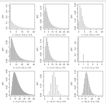
It is easy to verify that limx→∞G(x)=1. The plots of the PMF of the KGD for various values ofα,βandqare given in Figure 1.
3 Some properties of Kumaraswamy-geometric distribution
SupposeXfollows the KGD with CDFG(x)in (9). The quantile functionX∗(=Q(U), 0< U<1)of KGD is the inverse of the cumulative distribution. That is,
X∗=Q(U)=(logq)−1log
1− 1−(1−U)1/β1/α
0 5 10 15 20
0.0
0.1
0.2
0.3
0.4
α =0.2, β =0.2, q=0.3
g(x)
0 5 10 15 20 25 30
0.00
0.05
0.10
0.15
α =2,β =0.2, q=0.3
g(x)
0 5 10 15 20
0.00
0.10
0.20
0.30
α =5,β =0.5, q=0.3
g(x)
0 10 20 30 40
0.00
0.04
0.08
α =2,β =0.2, q=0.5
g(x)
0 5 10 15 20 25 30
0.00
0.05
0.10
0.15
α =5,β =0.5, q=0.5
g(x)
0 1 2 3 4 5
0.0
0.2
0.4
0.6
α =2,β =5,q=0.5
g(x)
0 10 20 30 40 50
0.00
0.02
0.04
0.06
α =5,β =0.5, q=0.8
g(x)
0 5 10 15
0.00
0.10
0.20
α =10, β =10, q=0.8
g(x)
0 5 10 20 30
0.00
0.04
0.08
0.12
α =20, β =2,q=0.8
g(x)
Figure 1 Probability mass function for values ofα,βandq.
whereUhas a uniform distribution with support on(0, 1). Equation (14) can be used to simulate the Kumaraswamy-geometric random variable. First, simulate a random vari-ableU and compute the value of X∗ in (14), which is not necessarily an integer. The Kumaraswamy-geometric random variateX is the largest integer ≤ X∗, which can be denoted by [X∗].
Transformation: The relationship between the KGD and the Kumaraswamy’s, exponen-tial, exponentiated-exponenexponen-tial, Pareto, Weibull, Rayleigh, and the logistic distributions are given in the following lemma.
Lemma 1.Suppose[v]denotes the largest integer less than or equal to the quantity v.
(a) IfY has Kumaraswamy’s distribution with parametersαandβ, then the distribution ofX=
logq(1−Y)
is KGD.
(b) IfY is standard exponential, thenX=
logq1−1−e−Y/β1/α
has KGD. (c) IfY follows an exponentiated-exponential distribution with scale parameterλand
index parameterc, thenX=
logq
1− 1−(1−e−λY)c/β1/α
(d) If the random variableYhas a Pareto distribution with parametersθ,kand CDF
F(y)=1−θ+θyk, thenX=
logq
1−
1−θ+θYk/β
1/α
has KGD.
(e) If the random variableYhas a Weibull distribution withF(y)=1−exp{−(y/γ )c} as CDF, thenX=
logq1−(1−exp[−(Y/γ )c/β])1/αhas KGD.
(f) If the random variableYhas a Rayleigh distribution withF(y)=1−exp
−
y2
2b2
as
CDF, thenX=
logq
1−
1−exp
−Y2
2b2β
1/α
has KGD.
(g) IfYis a logistic random variable withF(y)= 1+exp({−(y−a)/b})−1as CDF,
thenX=
logq
1−
1− 1+exp{−(Y−a)/b}−1/β
1/α
has KGD.
Proof.By using the transformation technique, it is easy to show that the random variable Xhas KGD as given in (10). We will show the result for part (a). LetRbe the CDF of the Kumaraswamy’s distribution.
P(X=x) = P
logq(1−Y)=x
=P
x≤logq(1−Y) <x+1
= P1−qx≤Y<1−qx+1=R1−qx+1−R1−qx = 1−(1−qx)αβ−1−1−qx+1αβ,
which is the PMF of the KGD in (10).
In general, if we have a continuous random variableYand its CDF isF(y), thenX =
logq
1−1−F1/β(Y)1/α
has KGD.
Limiting behavior: Asx→ ∞, limx→∞g(x)=0. Also, asx→0, limx→0g(x)=1−[1− (1−q)α]β. This limit becomes 0 ifq →1 and/orα → ∞. Thus, the distribution starts with probability zero or a constant probability as evident from Figure 1.
Mode of the KGD: Since the KGD is also LKGD, aT-geometric distribution, we use Lemma 2 in Alzaatrehet al. (2012b), which states that aT-geometric distribution has a reversed J-shape if the distribution of the random variableT has a reversed J-shape. We only need to show when the distribution of log-Kumaraswamy distribution has a reversed J-shape.
On taking the first derivative of (11) with respect tot, we obtain
f(t)= αe−t−1+1−e−tα−αβe−t1−e−tαV(t)=Q(t)V(t), (15)
whereV(t) = αβe−t1−e−tα−2 1−1−e−tαβ−2is positive. Forβ ≥ 1 andα ≤ 1, it is straight forward to show thatQ(t) ≤ 0. Forβ < 1 andα ≤ 1, the functionQ(t)is an increasing function oft. It is not difficult to show that limt→0Q(t) =α−1 ≤0 and
limt→∞Q(t)=0. Thus, forα ≤1 and any value ofβ andq,Q(t)≤0 and so the PDF of the log-Kumaraswamy distribution is monotonically decreasing or has a reversed J-shape. Hence, the KGD has a reversed J-shape and a unique mode atx=0 whenα≤1.
4 Moments
Using Equation (10), therthraw moment is given by
EXr=μr = ∞
x=1
xr1−1−qxαβ− ∞
x=1
xr1−1−qx+1αβ
= ∞
x=1 xr
⎡ ⎣
∞
i=1 (−1)i−1
α i qxi β − ∞
i=1 (−1)i−1
α
i
q(x+1)i
β⎤
⎦.
The two inner summations terminate atα, ifαis a positive integer. Whenβ =1 in the above, we have,
μr= ∞
x=1 xr
α
i=1 (−1)i−1
α
i
qxi(1−qi), for α∈Z+.
In particular, letr= 1 andα= 1, the expression for the first moment, or the mean of the KGD may be written as,
E(X)=μ1=q(1−q) ∞
x=1
xqx−1= q p,
which is the mean of the geometric distribution, a special case of KGD.
We discuss in what follows, an alternative approach of expressing the PMF of the KGD in Equation (10).
g(x) = 1−1−qxαβ−
1−1−qx+1α
β
= ∞
i=0 (−1)i
β
i 1−q
xαi−∞
i=0 (−1)i
β
i 1−q x+1αi
= ∞
i=0 (−1)i
β
i
∞
j=0 (−1)j
αi
j
qxj− ∞
i=0 (−1)i
β
i
∞
j=0 (−1)j
αi
j
q(x+1)j
= ∞
i=1 ∞
j=1 (−1)i+j
β i α i j
(1−qj)qxj. (16)
Using Equation (16), it is now easy to write the expressions for the moment, moment generating function, and probability generating function for the KGD respectively as follows:
μr= ∞
x=0 ∞
i=1 ∞
j=1 (−1)i+j
β i
αi
j 1−q
jxrqjx; !!qj!!<1, (17)
M(t)= ∞
x=0 ∞
i=1 ∞
j=1 (−1)i+j
β i
αi j 1−q
j etqjx; !!etqj!!<1, (18)
ϕ(t)= ∞
x=0 ∞
i=1 ∞
j=1 (−1)i+j
β
i
αi
j 1−q
j tqjx; !!tqj!!<1. (19)
series in (17) is absolutely convergent. Thus, interchanging the order of summation has no effect. Using Equation (17), therthmoment may be written as
E(Xr)=μ r =
∞
x=0 ∞
i=1 ∞
j=1 (−1)i+j
β i
αi
j 1−q
j qjxxr
= ∞
i=1 ∞
j=1 (−1)i+j
β
i
αi
j 1−q j
∞
x=1
qjxxr
= ∞
i=1 ∞
j=1
(−1)i+jβ
(i)
i! (αi)(j)
j!
1−qjL−r
qj,
whereβ(i)=β(β−1)(β−2)· · ·(β−i+1), and similarly for(αi)(j). Also,
L−r(u)= ∞
k=1 uk
k−r, u=q j,
is the polylogarithm function, (http://mathworld.wolfram.com/Polylogarithm.html). Expressions for the first few moments are thus:
μ1 = ∞
i=1 ∞
j=1
(−1)i+jβ
(i)
i! (αi)(j)
j! qj
1−qj, (20)
μ
2 =
∞
i=1 ∞
j=1
(−1)i+jβ
(i)
i! (αi)(j)
j!
qj1+qj
1−qj2 , (21)
μ3 = ∞
i=1 ∞
j=1
(−1)i+jβ
(i)
i! (αi)(j)
j!
qj1+4qj+q2j
(1−qj)3 , (22)
μ
4 =
∞
i=1 ∞
j=1
(−1)i+jβ
(i)
i! (αi)(j)
j!
qj1+qj 1+10qj+q2j
1−qj4 . (23)
The expression for the variance may be written as
σ2= ∞
i=1 ∞
j=1
(−1)i+jβ
(i)
i! (αi)(j)
j!
qj1+qj
1−qj2 −
⎛ ⎝∞
i=1 ∞
j=1
(−1)i+jβ
(i)
i! (αi)(j)
j! qj 1−qj
⎞ ⎠
2
.
Expressions for the skewness and kurtosis for the KGD may be obtained by combining appropriate expressions in Equations (20), (21), (22), and (23). In the particular case for whichα=1=β, the expressions for the central moments of the geometric distribution are as follows:
μ1=μ1= q
p, μ2=σ
2= q
p2, μ3=
q(1+q)
p3 , μ4=
qp2+9q
p4 .
The results for this special case may be found in standard textbooks on probability. See for example, Zwillinger and Kokoska (2000).
Both the moment generating function (M(t)) and the probability generating function (ϕ(t)) can be simplified further. In the case ofϕ(t), we have
ϕ(t)= ∞
i=1 ∞
j=1 (−1)i+j
β
i
αi
j 1−q j
∞
x=0
After further simplification, the above reduces to,
ϕ(t)= ∞
i=1 ∞
j=1 (−1)i+j
β
i
αi
j
(
1−qj) (1−tqj).
By letting
A(α,β|i,j)= ∞
i=1 ∞
j=1 (−1)i+j
β
i
α
i j
,
the first two factorial moments may be expressed as
ϕ(t=1) = μ[1]=E(X)=A(α,β|i,j) qj 1−qj
ϕ(t=1) = μ[2]=E(X(X−1))=A(α,β|i,j)
2q2j (1−qj)2.
In general,
ϕ(m)(t)=A(α,β|i,j)m!(1−qj)qmj (1−tqj)m+1 ,
which reduces to the result in Alzaatrehet al. (2012b) whenβ=1.
Through numerical computation, we obtain the mode, the mean, the standard deviation (SD), the skewness and the kurtosis of the KGD. The values ofαandβ for the numeri-cal computation are from 0.2 to 10 at an increment of 0.1, while the values ofqare from 0.2 to 0.9 at an increment of 0.1. For brevity, we report the mode, the mean and the stan-dard deviation in Table 1 and the skewness and kurtosis in Table 2 for some values of q, β andα. From the numerical computation, the mean, mode and standard deviation are increasing functions ofq. From Table 1, the mean, mode and standard deviation are decreasing functions ofβbut increasing functions ofα. Forα≤1, the skewness and kur-tosis are decreasing functions ofqbut increasing functions ofβ. Forα >1, the skewness and kurtosis first decrease and then increase as bothqandβincrease. The skewness and kurtosis are decreasing functions ofα. Some of these observations can be seen in Table 2 while others are from the numerical computation. Instead of Tables 1 and 2, contour plots may be used to present the results in the tables. However, it becomes difficult to see the patterns described above.
5 Hazard rate and Shannon entropy
The hazard rate function is defined as
h(x)= g(x) 1−G(x),
whereG(x) = xy=0g(y). For the KGD, we have, after substituting expressions for the PMF and CDF (Equations (10) and (9)),
h(x)=
1−(1−qx)α 1−1−qx+1α
β
−1. (24)
The asymptotic behaviors of the hazard function are such that,
lim
x→0h(x)=(1−p
α)−β−1=L
1,
Table 1 Mode, mean and standard deviation (SD) of KGD for some values ofα,βandq
q=0.4 q=0.6 q=0.8
α β Mode Mean SD Mode Mean SD Mode Mean SD
0.4 0.4 0 1.60 2.48 0 3.16 4.51 0 7.74 10.40
0.6 0 0.83 1.52 0 1.72 2.81 0 4.39 6.54
0.8 0 0.48 1.04 0 1.06 1.96 0 2.82 4.60
1.5 0 0.10 0.39 0 0.29 0.79 0 0.92 1.96
2.0 0 0.04 0.22 0 0.13 0.49 0 0.49 1.26
4.0 0 0.001 0.04 0 0.01 0.11 0 0.07 0.35
0.6 0.4 0 1.87 2.59 0 3.67 4.69 0 8.97 10.80
0.6 0 1.04 1.65 0 2.14 3.02 0 5.43 6.99
0.8 0 0.64 1.17 0 1.41 2.18 0 3.71 5.08
1.5 0 0.18 0.51 0 0.48 1.00 0 1.48 2.42
2.0 0 0.08 0.32 0 0.26 0.67 0 0.91 1.67
4.0 0 0.005 0.07 0 0.04 0.20 0 0.21 0.62
0.8 0.4 0 2.08 2.66 0 4.08 4.81 0 9.93 11.04
0.6 0 1.21 1.74 0 2.49 3.16 0 6.27 7.27
0.8 0 0.79 1.27 0 1.71 2.33 0 4.47 5.38
1.5 0 0.26 0.60 0 0.68 1.16 0 2.01 2.74
2.0 0 0.13 0.40 0 0.41 0.82 0 1.35 1.99
4.0 0 0.01 0.12 0 0.08 0.31 0 0.43 0.87
1.5 0.4 1 2.61 2.79 1 5.06 5.00 3 12.22 11.44
0.6 0 1.68 1.89 1 3.39 3.39 2 8.38 7.76
0.8 0 1.21 1.44 1 2.54 2.59 2 6.43 5.92
1.5 0 0.54 0.81 0 1.31 1.47 1 3.61 3.35
2.0 0 0.35 0.62 0 0.95 1.14 1 2.77 2.61
4.0 0 0.08 0.29 0 0.38 0.63 0 1.42 1.46
2.0 0.4 1 2.87 2.83 2 5.55 5.06 4 13.35 11.57
0.6 1 1.93 1.94 1 3.85 3.47 4 9.45 7.92
0.8 1 1.44 1.50 1 2.97 2.68 3 7.45 6.10
1.5 0 0.73 0.89 1 1.69 1.58 2 4.51 3.57
2.0 0 0.51 0.71 1 1.30 1.26 2 3.61 2.83
4.0 0 0.18 0.40 0 0.65 0.77 1 2.11 1.69
4.0 0.4 2 3.56 2.89 3 6.79 5.16 8 16.19 11.79
0.6 1 2.59 2.02 3 5.05 3.59 7 12.21 8.19
0.8 1 2.09 1.59 2 4.14 2.81 6 10.13 6.41
1.5 1 1.32 1.01 2 2.77 1.74 5 7.00 3.94
2.0 1 1.08 0.84 2 2.34 1.43 4 5.99 3.23
4.0 1 0.64 0.61 1 1.57 0.96 3 4.24 2.10
6.0 0.4 2 3.99 2.90 4 7.55 5.19 10 17.92 11.87
0.6 2 3.01 2.04 4 5.79 3.63 9 13.90 8.29
0.8 2 2.50 1.61 3 4.87 2.86 8 11.80 6.53
1.5 1 1.72 1.03 3 3.47 1.80 7 8.59 4.08
2.0 1 1.46 0.87 2 3.02 1.50 6 7.55 3.38
4.0 1 1.02 0.62 2 2.21 1.02 5 5.71 2.27
the hazard rate function for the EEGD discussed in Alzaatrehet al. (2012b). Observe that L1 > L2 when α < 1. Forα < 1, we check the behavior of h(x). The function h(x)
Table 2 Skewness and kurtosis of KGD for some values ofα,βandq
q=0.4 q=0.6 q=0.8
α β Skewness Kurtosis Skewness Kurtosis Skewness Kurtosis
0.4 0.4 2.4529 8.4883 2.3789 8.0612 2.3360 7.8215
0.6 2.8022 10.920 2.6534 9.9332 2.5656 9.3787
0.8 3.1918 14.035 2.9430 12.172 2.7954 11.133
1.5 4.9662 32.736 4.0792 23.245 3.5894 18.553
2.0 6.8722 60.013 5.0708 35.519 4.1724 25.214
4.0 30.524 990.63 12.671 196.82 7.1320 72.567
0.6 0.4 2.2480 7.2663 2.1956 7.0004 2.1684 6.8666
0.6 2.4465 8.4649 2.3387 7.8659 2.2823 7.5649
0.8 2.6694 9.9363 2.4883 8.8459 2.3932 8.3020
1.5 3.6723 17.839 3.0582 13.119 2.7529 10.999
2.0 4.6998 27.856 3.5337 17.209 2.9979 13.043
4.0 14.964 238.38 6.6621 54.450 4.0916 23.691
0.8 0.4 2.1208 6.5743 2.0847 6.4108 2.0685 6.3383
0.6 2.2269 7.1361 2.1498 6.7675 2.1151 6.6063
0.8 2.3522 7.8283 2.2198 7.1642 2.1603 6.8772
1.5 2.9553 11.535 2.5010 8.8497 2.3055 7.8006
2.0 3.5861 16.072 2.7466 10.413 2.4048 8.4499
4.0 9.2202 90.141 4.3332 22.881 2.8543 11.487
1.5 0.4 1.9024 5.5182 1.9015 5.5273 1.9038 5.5384
0.6 1.8485 5.2051 1.8400 5.2063 1.8433 5.2269
0.8 1.8105 4.9322 1.7862 4.9087 1.7894 4.9374
1.5 1.8191 4.4671 1.6645 4.1552 1.6529 4.1894
2.0 1.9494 4.6197 1.6281 3.8307 1.5890 3.8375
4.0 3.3608 11.0492 1.7629 3.5961 1.4574 3.0767
2.0 0.4 1.8322 5.2176 1.8440 5.2733 1.8503 5.2983
0.6 1.7260 4.6855 1.7442 4.7835 1.7563 4.8321
0.8 1.6352 4.2020 1.6551 4.3386 1.6733 4.4121
1.5 1.4620 3.0364 1.4309 3.2239 1.4664 3.3814
2.0 1.4564 2.6068 1.3301 2.7152 1.3700 2.9254
4.0 2.0958 3.6392 1.1838 1.6496 1.1546 1.9922
4.0 0.4 1.7344 4.8228 1.7559 4.9001 1.7627 4.9251
0.6 1.5605 4.0589 1.6019 4.1951 1.6151 4.2403
0.8 1.4043 3.3984 1.4675 3.5897 1.4874 3.6530
1.5 1.0049 1.9031 1.1406 2.2381 1.1833 2.3432
2.0 0.8155 1.2870 0.9925 1.7112 1.0500 1.8310
4.0 0.4669 −0.1633 0.6666 0.8077 0.7728 0.9349
6.0 0.4 1.7069 4.7081 1.7246 4.7731 1.7310 4.7964
0.6 1.5197 3.8941 1.5522 4.0017 1.5641 4.0428
0.8 1.3558 3.2107 1.4034 3.3521 1.4207 3.4078
1.5 0.9572 1.7788 1.0513 1.9565 1.0843 2.0406
2.0 0.7743 1.2870 0.8984 1.4383 0.9394 1.5299
4.0 0.3102 0.6548 0.5863 0.5921 0.6444 0.6837
hazard rate whenα < 1 and an increasing hazard rate whenα > 1. Forα = 1,L1 = L2and we have a constant hazard rate. The graphs of the hazard rate function defined
in Equation (24) are shown in Figure 2 for various values of the parameters. We see in Figure 2 that the hazard rate decreases for values ofα <1 and increases forα >1.
The entropy of a random variable is a measure of variation of uncertainty. For a discrete random variableXwith probability mass functiong(x), the Shannon entropy is defined as,
S(x)= − x
g(x)log2g(x)≥0. (25)
In probabilistic context, S(x) is a measure of the information carried by g(x), with higher entropy corresponding to less information. Substituting Equation (10) in Equation (25), we have
S(x) = − x
[1−(1−qx)α]β−
1−1−qx+1α
β
×log2
[1−(1−qx)α]β−
1−1−qx+1α
β
.
Suppose we write the PMF as
[1−(1−qx)α]β
⎧ ⎨ ⎩1−
1−1−qx+1α
1−(1−qx)α
β⎫⎬
⎭.
10 15
0.25
0.30
0.35
α=0.75, β=0.75, q=0.75
h
(
x
)
0 5 0 5 10 15
0.
8
0
.9
1.
0
1
.1
1.
2
1
.3
1.
4
α=0.75, β=2, q=0.75
h
(
x
)
0 5 10 15
1.
.5
2.0
0
1
2.5
3.0
α=2, β=2, q=0.5
h
(
x
)
0 5 10 15 20 25 30
0.
0
1.0
2.
0
3.0
α=5, β=5, q=0.75
h
(
x
)
Letα=1 for simplicity. We may now write the entropy as
S(x)= − ∞
x=0
1−qβqxβlog21−qβqxβ. (26)
After some algebra, Equation (26) becomes,
S(x)= −
1−qβlog21−qβ−qβlog2qβ
1−qβ >0. (27)
On settingβ=1 in Equation (27), we have, for the geometric distribution,
S(x)= − q
1−qlog2q−log2(1−q)=
−(1−p)log2(1−p)−plog2p
p .
Note that whenβ=1, p=q=1/2,S(x)=2. It is not difficult to show thatS(x)is an increasing function ofqfor any givenβ. This is consistent with the pattern of the standard deviation. We also note that limβ→∞S(x) = 0, with the proviso that 0 log 0 = 0. This indicates that smaller values ofβincrease the uncertainty in the distribution, while higher values of β increase the amount of information measured in terms of the probability. Actually, a zero entropy indicates that all information needed is measured solely in terms of the probability. In a way, the KGD has smaller entropy (more probabilistic information) than the geometric distribution for values ofβ >1.
6 Maximum likelihood estimation
We discuss the maximum likelihood estimation of the parameters of the KGD in subsection 6.1. Subsection 6.2 contains the results of a simulation that is conducted to evaluate the performance of the maximum likelihood estimation method.
6.1 Estimation
Let a random sample of sizenbe taken from KGD, with observed frequenciesnx, x = 0, 1, 2,. . .,k, where kx=0nx = n. From Equation (10), the likelihood function for a random sample of sizenmay be expressed as
L(x|α,β,q)= k
,
x=0
1−1−qxαβ−
1−1−qx+1α
βnx
. (28)
The log-likelihood function is
l(α,β,q)=lnL(x|α,β,q)=n0ln
1− 1−(1−q)αβ
+ k
x=1
nxln 1−1−qxαβ−
1−1−qx+1α
β
.
Differentiating the log-likelihood function with respect to the parameters, we obtain
∂l(α,β,q) ∂α =
n0β(1−q)α 1−(1−q)α
β−1
ln(1−q)
1− 1−(1−q)αβ
+ k
x=1
nx[Ax+Bx]
1−(1−qx)αβ−1−1−qx+1αβ, (30)
∂l(α,β,q) ∂β =
−n0 1−(1−q)α
β
ln 1−(1−q)α
1− 1−(1−q)αβ
+ k
x=1
nx[Cx−Dx]
1−(1−qx)αβ−1−1−qx+1αβ, (31)
∂l(α,β,q) ∂q =
−n0αβ 1−(1−q)α
β−1
(1−q)α−1 1−[1−(1−q)α]β
+ k
x=1
nx[Ex−Fx]
1−(1−qx)αβ−1−1−qx+1αβ, (32)
where,
Ax = −β 1−1−qxαβ−11−qxαln1−qx,
Bx = β
1−1−qx+1α
β−1
1−qx+1αln1−qx+1,
Cx = 1−
1−qxαβln 1−1−qxα,
Dx =
1−1−qx+1αβln1−1−qx+1α,
Ex = αβxqx−1 1−
1−qxαβ−11−qxα−1,
Fx = αβ (x+1)qx
1−1−qx+1α
β−1
1−qx+1α−1.
Setting the non-linear Equations (30), (31) and (32) to zero and solving them iteratively, we get the estimatesθˆ = (αˆ,βˆ,qˆ)T for the parameter vectorθ = (α,β,q)T. The initial values of parametersαandβcan be set to 1 and that of parameterqcan be set to 0.5.
For interval estimation and hypothesis tests on the parameters, we require the infor-mation matrix I(θ), with elements−∂2l/(∂i∂j) = −lij, where,i,j ∈ {α,β,q}. Under conditions that are fulfilled for parameters in the interior of the parameter space but not on the boundary, the asymptotic distribution of√n(θˆ−θ) is N3(0,I−1(θ)). The
asymptotic multivariate normal distributionN3(0,I−1(θ))ˆ ofθˆcan be used to construct
approximate confidence intervals for the parameters. For example, the 100(1 − ξ)% asymptotic confidence interval for theithparameterθiis given by
ˆ
θi−zξ/2-Ii,i, θiˆ +zξ/2-Ii,i
,
The information matrixI(θ)is of the form,
I(α,β,q)=
⎛ ⎜ ⎝
lαα lαβ lαq lβα lββ lβq lqα lqβ lqq
⎞ ⎟ ⎠.
The expressions for the elementslijare given in the Appendix.
6.2 Simulation
A simulation study is conducted to evaluate the performance of the maximum likelihood estimation method. Equation (14) is used to generate a random sample from the KGD with parametersα,βandq. The different sample sizes considered in the simulation are n=250, 500 and 750. The parameter combinations for the simulation study are shown in Table 3. The combinations were chosen to reflect the following cases of the distribution: under-dispersion (α = 6, β = 4, q = 0.8), over-dispersion (all other cases), monoton-ically decreasing (α = 1.6, β = 2.0, q = 0.6), and unimodal with mode greater than 0 (all other cases). For each parameter combination and each sample size, the simulation process is repeated 100 times. The average bias (actual−estimate) and standard devi-ation of the parameter estimates are reported in Table 3. The biases are relatively small when compared to the standard deviations. In most cases, as the sample size increases, the standard deviations of the estimators decrease.
7 Applications of KGD
We apply the KGD to two data sets. The first data set is the observed frequencies of the distribution of purchases of a brandXbreakfast cereals purchased by consumers over a period of time (Consul 1989). The other data set is the number of absences among shift-workers in a steel industry (Gupta and Ong 2004). Comparisons are made with the generalized negative binomial distribution (GNBD) defined by Jain and Consul (1971) and
Table 3 Bias and standard deviation for maximum likelihood estimates
Actual values Bias with standard deviation in parentheses
n α β q αˆ βˆ qˆ Mode
250 1.6 2.0 0.6 −0.1295(0.2099) 0.1128(0.4697) 0.0409(0.0733) 0
4.0 2.0 0.4 −0.3136(0.7844) 0.1047(0.4617) 0.0237(0.0698) 1
4.0 2.0 0.6 −0.1977(0.5714) 0.1021(0.4571) 0.0198(0.0571) 2
4.0 2.0 0.8 −0.2467(0.5521) 0.0852(0.4020) 0.0126(0.0293) 4
6.0 4.0 0.8 −0.3931(0.8570) 0.2084(0.9507) 0.0121(0.0278) 5
500 1.6 2.0 0.6 −0.0437(0.1436) 0.0121(0.4496) 0.0153(0.0665) 0
4.0 2.0 0.4 −0.3142(0.5876) 0.1383(0.4421) 0.0290(0.0639) 1
4.0 2.0 0.6 −0.2015(0.4728) 0.0808(0.4504) 0.0194(0.0527) 2
4.0 2.0 0.8 −0.2747(0.4630) 0.1526(0.3781) 0.0157(0.0278) 4
6.0 4.0 0.8 −0.3283(0.7771) 0.2187(0.9375) 0.0116(0.0267) 5
750 1.6 2.0 0.6 −0.0533(0.1305) 0.1184(0.4250) 0.0278(0.0669) 0
4.0 2.0 0.4 −0.3181(0.5939) 0.1707(0.4195) 0.0328(0.0622) 1
4.0 2.0 0.6 −0.1787(0.4775) 0.0562(0.4469) 0.0159(0.0522) 2
4.0 2.0 0.8 −0.1717(0.4739) 0.0813(0.4117) 0.0101(0.0299) 4
the exponentiated-exponential geometric distribution (EEGD) defined by Alzaatrehet al. (2012b).
7.1 Purchases by consumers
Consul (1989), p. 128 stated that, “The number of units of different commodities pur-chased by consumers over a period of time”, appears to follow the generalized Poisson distribution (GPD). In support of this assertion, the author analyzed some relevant data sets and observed that the GPD model provided adequate fits. One of the data sets consid-ered by Consul (1989) consists of observed frequencies of the distribution of purchases of a brandXbreakfast cereals. The original data in Table 4 was taken from Chatfield (1975). The data contains the frequency of consumers who boughtr units of brandX over a number of weeks. The data is fitted to the KGD, EEGD, and the GNBD. We are not sure how the frequencies for the (10-11), (12-15) and (16-35) were handled in previous applications of the data set. In our analysis, the probabilities for the classes (10-11) and (12-15) were obtained by adding the corresponding individual probabilities in each class. When finding the maximum likelihood estimates, the probability for the last class was obtained by subtracting the sum of all previous probabilities from 1. The results in Table 4 show that all the three distributions provide adequate fit to the data. Since the parameter β in KGD is not significantly different from 1, it may be more appropriate to apply the two-parameter EEGD to fit the data. Also, the likelihood ratio test to compare the EEGD with the KGD is not significant at 5% level.
Table 4 The number of unitsrpurchased by observed number (fr) of consumers
Expected
r-value Observed EEGD GNBD KGD
0 299 300.11 298.98 299.33
1 69 63.10 68.03 65.59
2 37 41.13 41.12 42.02
3 34 30.68 29.89 30.92
4 23 24.36 23.51 24.28
5 20 20.06 19.32 19.81
6 12 16.92 16.32 16.58
7 18 14.52 14.04 14.14
8 14 12.61 12.25 12.21
9 9 11.06 10.80 10.67
10-11 17 18.47 18.16 17.72
12-15 27 26.69 26.63 25.50
16-35 63 62.29 62.95 63.23
Total 642 642 642 642
Parameter αˆ=0.2910(0.0212) θˆ=0.9658(0.0148) αˆ=0.3373(0.0924) Estimates θˆ=0.9267(0.0076) mˆ =0.2264(0.0339) βˆ=1.5114(1.3648)
ˆ
β=0.9882(0.0126) qˆ=0.9592(0.0544)
χ2 4.34 3.92 4.11
df 10 9 9
p-value 0.9307 0.9166 0.9040
AIC 2471.3 2472.8 2473.0
LL∗ −1233.64 −1233.38 −1233.50
7.2 Number of absences by shift-workers
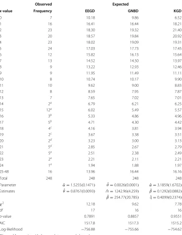
The KGD is also applied to a data set from Gupta and Ong (2004), which represents the observed frequencies of the number of absences among shift-workers in a steel industry. The data in Table 5 was originally studied by Arbous and Sichel (1954) in an attempt to create a model that can describe the distribution of absences to a group of people in single- and double-exposure periods. The original data contains the number of absences, x-value, of 248 shift workers in the years 1947 and 1948. Arbous and Sichel (1954) used the negative binomial distribution (NBD) to fit the data. Gupta and Ong (2004) proposed a four-parameter generalized negative binomial distribution to fit the data and compared it to the NBD and the GPD. The chi-square value for their distribution was 8.27 with 15
Table 5 The number of absences among shift-workers in a steel industry
Observed Expected
x-value Frequency EEGD GNBD KGD
0 7 10.18 9.86 6.52
1 16 16.41 16.44 18.21
2 23 18.30 19.32 21.40
3 20 18.57 19.84 20.92
4 23 18.02 19.09 19.31
5 24 17.03 17.73 17.45
6 12 15.82 16.13 15.64
7 13 14.52 14.50 13.97
8 9 13.22 12.93 12.46
9 9 11.95 11.49 11.11
10 8 10.74 10.17 9.90
11 10 9.62 9.00 8.83
12 8 8.59 7.95 7.87
13 7 7.65 7.02 7.01
14 2a 6.79 6.21 6.25
15 12a 6.02 5.49 5.57
16 3b 5.33 4.86 4.96
17 5b 4.71 4.30 4.42
18 4c 4.16 3.81 3.94
19 2c 3.67 3.38 3.51
20 2d 3.23 3.00 3.13
21 5d 2.85 2.67 2.79
22 5e 2.51 2.38 2.49
23 2e 2.21 2.11 2.21
24 1e 1.94 1.88 1.97
25-48 16 13.96 16.44 16.16
Total 248 248 248 248
Parameter αˆ=1.5255(0.1471) θˆ=0.0026(0.0001) αˆ=3.1859(1.6702) Estimates θˆ=0.8767(0.0093) mˆ =1242.96(4.259) βˆ=0.1292(0.0882)
ˆ
β=254.77(20.785) qˆ=0.4099(0.2374)
χ2 12.18 9.62 7.78
df 17 16 16
p-value 0.7891 0.8857 0.9551
AIC 1517.8 1517.3 1515.2
Log-likelihood −756.88 −755.66 −754.62
degrees of freedom. The chi-square value obtained by Gupta and Ong for the GPD was 27.79 with 17 degrees of freedom (DF). The DF= k−s−1, wherekis the number of classes andsis the number of estimated parameters.
We re-analyzed the data for the EEGD, the GNBD, and the GPD. We obtained a chi-square of 9.62 for the GPD, which is much smaller than the 27.79 provided by Gupta and Ong. Thus, our estimates from the GPD (not reported in Table 5) differ significantly from the results in Gupta and Ong (2004). When finding the maximum likelihood estimates, the probability for the last class was obtained by subtracting the sum of all previous prob-abilities from 1. In view of this, the results obtained from the EEGD are slightly different from those of Alzaatrehet al. (2012b) who applied the EEGD to fit the data. We apply the KGD to model the data in Table 5, and the results from the table indicate that the KGD, EEGD and GNBD provide good fit to the data.
Ifm→ ∞, the GNBD with parametersθ,mandβgoes to the GPD with parametersα andλ, whereα = mθ andλ = θβon page 218 of Consul and Famoye (2006). We fitted the GPD to the data and we got the same log-likelihood withαˆ =3.2250 andλˆ =0.6597. From the GNBD, we obtainedmˆθˆ = 1242.96×0.002591 = 3.22 ≈ 3.2250 = ˆα and
ˆ
βθˆ=254.77×0.002591=0.66≈0.6597= ˆλ.
We observe that the parameterβ in the KGD is significantly different from 1. This makes the KGD a more appropriate distribution over the EEGD. The likelihood ratio statistic for testing the EEGD against the KGD isχ12 = −2(754.62−756.88) = 4.52 with ap-value of 0.0335. Thus, we reject the null hypothesis that the data follows the EEGD at the 5% level. The likelihood ratio test supports the claim that the parameterβis significantly different from 1, and hence the KGD appears to be superior to the EEGD.
8 Conclusion
Discrete distributions are often derived by using the Lagrange expansions framework (see for example Consul and Famoye 2006) or using difference equations (see for example Johnsonet al. 2005). Recently, Alzaatrehet al. (2012b, 2013b) developed a general method for generating distributions and these distributions are members of theT-Xfamily. The method can be applied to derive both the discrete and continuous distributions. This article used theT-Xfamily framework to define a new discrete distribution named the Kumaraswamy-geometric distribution (KGD).
Appendix
Elements of the information matrix
lα α = A0 1−β(1−q)
αln(1−q)
P0 1−(1−q)α
−A0B0 P20 +
k
x=1 nx Px
∂ (Ax+Bx) ∂α −
(Ax+Bx)2 Px
,
lα β = A0 P0β +
A0ln 1−(1−q)α
P20 +
k
x=1 nx Px
∂ (Ax+Bx) ∂β −
(Ax+Bx) (Cx−Dx) Px
,
lαq = A0 P0
α{β(1−q)α−1+ 1−(1−q)αβ} (1−q) 1−(1−q)αP0 −
1 (1−q)ln(1−q)
+ k
x=1 nx Px
∂ (Ax+Bx)
∂q −
(Ax+Bx) (Ex−Fx) Px
,
lβ β = C0ln 1−(1−q) α
P20 +
k
x=1 nx Px
∂(Cx−Dx) ∂β −
(Cx−Dx)2 Px
,
lβq = C0 P0
αβ(1−q)α−1 1−(1−q)αP0
+ α(1−q)α−1
1−(1−q)αln 1−(1−q)α
+ k
x=1 nx Px
∂ (Cx−
Dx) ∂q −
(Cx−Dx) (Ex−Fx) Px
,
lq q = E0 P0
αβ(1−q)α−1 1−(1−q)αβ−1
P0 +
(αβ−1) (1−q)α−α+1 (1−q) 1−(1−q)α
+ k
x=1 nx Px
∂ (Ex−Fx) ∂q −
(Ex−Fx)2 Px
,
where,
Px = 1−
1−qxαβ−1−1−qx+1αβ,
P0 = 1− 1−(1−q)αβ,
A0 = n0β(1−q)α 1−(1−q)α
β−1
ln(1−q),
B0 = β(1−q)α 1−(1−q)α
β−1
ln(1−q),
C0 = −n0 1−(1−q)α
β
ln 1−(1−q)α,
E0 = −n0αβ 1−(1−q)α
β−1(
1−q)α−1, ∂Ax
∂α =
Ax 1−β (1−qx)α
ln(1−qx) 1−(1−qx)α , ∂Ax
∂β = Ax
1/β+ln 1−1−qxα,
∂Ax ∂q =
Axαxqx−1 β (1−qx)α−1 (1−qx) 1−(1−qx)α −
Axxqx−1 (1−qx)ln(1−qx), ∂Bx
∂α =
Bx 1−β
1−qx+1αln1−qx+1 1−1−qx+1α , ∂Bx
∂β = Bx
1/β+ln
1−1−qx+1α
∂Bx ∂q =
Bxα(x+1)qx[β(1−qx+1)α−1] 1−qx+1 1−1−qx+1α −
Bx(x+1)qx
1−qx+1ln1−qx+1, ∂Cx
∂α =
−Cx(1−qx)αln(1−qx) 1−(1−qx)α
β+ 1
ln[1−(1−qx)α]
,
∂Cx
∂β = Cxln[1−(1−qx)α] , ∂Cx
∂q =
Cxαxqx−1(1−qx)α−1
1−(1−qx)α
β+ 1
ln[1−(1−qx)α]
,
∂Dx ∂α =
−Dx
1−qx+1αln1−qx+1 1−1−qx+1α
β+ 1
ln 1−1−qx+1α
,
∂Dx
∂β = Dxln
1−1−qx+1α
,
∂Dx ∂q =
Dxα(x+1)qx1−qx+1α−1 1−1−qx+1α
β+ 1
ln 1−1−qx+1α
,
∂Ex ∂α = Ex
1/α+ [1−β(1−q
x)α] ln(1−qx)
1−(1−qx)α
,
∂Ex ∂β = Ex
1/β+ln[1−(1−qx)α],
∂Ex ∂q =
Ex(x−1)
q +
Ex[(αβ−1)(1−qx)α−α+1]xqx−1 (1−qx)[1−(1−qx)α] , ∂Fx
∂α = Fx
1/α+ 1−β
1−qx+1αln1−qx+1 1−1−qx+1α
,
∂Fx ∂β = Fx
1/β+ln1−1−qx+1α, and
∂Fx ∂q =
Fxx
q +
Fx (αβ−1)1−qx+1α−α+1(x+1)qx
1−qx+1 1−1−qx+1α .
The values ofAx,Bx,Cx,Dx,Ex, andFxare given in Section 6.
Competing interests
The authors declare that they have no competing interests.
Authors’ contributions
The authors, viz AA, FF and CL with the consultation of each other carried out this work and drafted the manuscript together. All authors read and approved the final manuscript.
Acknowledgment
The authors are grateful to the Associate Editor and the anonymous referees for many constructive comments and suggestions that have greatly improved the paper.
Author details
1Department of Mathematics, Marshall University, Huntington, West Virginia 25755, USA.2Department of Mathematics, Central Michigan University, Mount Pleasant, Michigan 48859, USA.
Received: 4 February 2014 Accepted: 15 July 2014
References
Akinsete, A, Famoye, F, Lee, C: The beta-Pareto distributions. Statistics.42(6), 547–563 (2008)
Alexander, C, Cordeiro, GM, Ortega, EMM, Sarabia, JM: Generalized beta-generated distributions. Comput. Stat. Data Anal. 56, 1880–1897 (2012)
Alshawarbeh, E, Famoye, F, Lee, C: Beta-Cauchy distribution: some properties and its applications. J. Stat. Theory Appl. 12, 378–391 (2013)
Alzaatreh, A, Famoye, F, Lee, C: Weibull-Pareto distribution and its applications. Comm. Stat. Theor. Meth. 42(7), 1673–1691 (2013a)
Alzaatreh, A, Lee, C, Famoye, F: On the discrete analogues of continuous distributions. Stat. Meth.9, 589–603 (2012b) Alzaatreh, A, Lee, C, Famoye, F: A new method for generating families of continuous distributions. Metron.71, 63–79
(2013b)
Arbous, AG, Sichel, HS: New techniques for the analysis of asenteeism data. Biometrika.41, 77–90 (1954) Chatfield, C: A marketing application of characterization theorem. In: Patil, GP, Kotz, S, Ord, JK (eds.) Statistical
Distributions in Scientific Work, volume 2, pp. 175–185. D. Reidel Publishing Company, Boston, (1975) Consul, PC: Generalized Poisson Distributions: Properties and Applications. Marcel Dekker, Inc., New York (1989) Consul, PC, Famoye, F: Lagrangian Probability Distributions. Birkhäuser, Boston (2006)
Cordeiro, GM, de Castro, M: A new family of generalized distributions. J. Stat. Comput. Simulat.81(7), 883–898 (2011) Cordeiro, GM, Lemonte, AJ: The beta Laplace distribution. Stat. Probability Lett.81, 973–982 (2011)
Cordeiro, GM, Nadarajah, S, Ortega, EMM: The Kumaraswamy Gumbel distribution. Stat. Methods Appl.21, 139–168 (2012) de Pascoa, MAR, Ortega, EMM, Cordeiro, GM: The Kumaraswamy generalized gamma distribution with application in
survival analysis. Stat. Meth.8, 411–433 (2011)
de Santana, TV, Ortega, EMM, Cordeiro, GM, Silva, GO: The Kumaraswamy-log-logistic distribution. Stat. Theory Appl. 3, 265–291 (2012)
Eugene, N, Lee, C, Famoye, F: The beta-normal distribution and its applications. Comm. Stat. Theor. Meth.31(4), 497–512 (2002)
Famoye, F, Lee, C, Olumolade, O: The beta-Weibull distribution. J. Stat. Theory Appl.4(2), 121–136 (2005)
Gupta, RC, Ong, SD: A new generalization of the negative binomial distribution. Comput. Stat. Data Anal.45, 287–300 (2004)
Jain, GC, Consul, PC: A generalized negative binomial distribution. SIAM J. Appl. Math.21, 501–513 (1971) Johnson, NL, Kemp, AW, Kotz, S: Univariate Discrete Distributiuons. third edition. John Wiley & Sons, New York (2005) Jones, MC: Kumaraswamy’s distribution: a beta-type distribution with some tractability advantages. Stat. Methodologies.
6, 70–81 (2009)
Kong, L, Lee, C, Sepanski, JH: On the properties of of beta-gamma distribution. J. Mod. Appl. Stat. Meth.6(1), 187–211 (2007)
Kumaraswamy, P: A generalized probability density function for double-bounded random processes. Hydrology 46, 79–88 (1980)
Lemonte, AJ, Barreto-Souza, W, Cordeiro, GM: The exponentiated Kumaraswamy distribution and its log-transform. Braz. J. Probability Stat.27, 31–53 (2013)
Mahmoudi, E: The beta generalized Pareto distribution with application to lifetime data. Math. Comput. Simulations. 81, 2414–2430 (2011)
Nadarajah, S, Kotz, S: The beta Gumbel distribution. Math. Probl. Eng.2004(4), 323–332 (2004) Nadarajah, S, Kotz, S: The beta exponential distribution. Reliability Eng. Syst. Saf.91, 689–697 (2006)
Singla, N, Jain, K, Sharma, SK: The beta generalized Weibull distribution: properties and applications. Reliability Eng. Syst. Saf.102, 5–15 (2012)
Zwillinger, D, Kokoska, S: Standard Probability and Statistics Tables and Formulae. Chapman and Hall/CRC, Boca Raton (2000)
doi:10.1186/s40488-014-0017-1
Cite this article as:Akinseteet al.:The Kumaraswamy-geometric distribution.Journal of Statistical Distributions and Applications20141:17.
Submit your manuscript to a
journal and benefi t from:
7Convenient online submission 7Rigorous peer review
7Immediate publication on acceptance 7Open access: articles freely available online 7High visibility within the fi eld
7Retaining the copyright to your article