Analysis and optimization of a cone
flowmeter performance by means of a
numerical and experimental approach
Giuseppe Dinardo, Laura Fabbiano, and Gaetano Vacca
DMMM, Politecnico di Bari University, 70125 Bari, Italy
Correspondence:Giuseppe Dinardo ([email protected])
Received: 5 June 2019 – Revised: 10 August 2019 – Accepted: 12 August 2019 – Published: 2 September 2019
Abstract. Differential pressure flowmeters are commonly used in industrial applications where, however, the upstream flow conditions are usually highly disturbed, caused by the presence, in the network pipe, of elbows, valves, etc. To achieve accurate flow measurements, the use of the cone meter is recommended as the flowmeter has the property to normalize the flow both upstream and downstream. In this paper, the authors present a cone flowmeter of new geometry that allows them to obtain better performance with respect to the original one; in particular, it provides a higher discharge coefficient (Cd) for a wider range of operating conditions.
1 Introduction
Accurate flow measurements are required in many industry applications. The ability to accurately and cheaply measure the flow rate has, in fact, a significant economic impact upon operating costs in control and production processes of several industries. The obstruction flowmeters are commonly used in typical industrial applications. Examples are the orifice me-ter, the nozzle meme-ter, the Venturi meme-ter, and Pitot meter. Ori-fice devices are widely used due to their smaller size and low cost, but their lower discharge coefficient, along with occur-ring inaccuracies in the measurement, due to erosion and cor-rosion of the plates (Shah et al., 2012), means their choice is discouraged where the measurement accuracy is important. On the other hand, the nozzle and Venturi meters present higher discharge coefficients, and, therefore, the most accu-rate flow accu-rate evaluations.
The Venturi meters are, however, considerably larger, heavier, and more expensive than orifice plates. Their instal-lation is also tougher (Miller, 1996). To obtain accurate mea-surements of the flow rate the flow upstream of the device must be as undisturbed as possible. Unfortunately, the piping systems do not guarantee such conditions because of the un-avoidable presence of elbows, valves, junctions, and so forth (Ifft and Mikkelsen, 1993). Further, correct measurements of upstream and downstream pressures require that the
obstruc-tion device causes as low disturbances as possible on the rel-ative pressure fields (Prabu et al., 1996; Sapra et al., 2011).
In this paper, the authors investigate the performance en-sured by the cone flowmeter. In Prabu et al. (1996), an interesting study about the effect of upstream flow distur-bances on the value of the cone flowmeter discharge coeffi-cient is performed. Mainly for this reason, recently, the cone flowmeter has emerged as the most attractive choice for in-dustrial applications, able to measure the flow rate in accu-rate manner, even in the presence of disturb sources (Ifft and Mikkelsen, 1993), and presenting a discharge coefficient less sensitive to the Reynolds number (Hollingshead et al., 2011). Because of its characteristic shape, the cone meter has other merits, such as higher durability and higher resistance to the abrasion, compared to other differential pressure flowmeters (Ifft and Mikkelsen, 1993).
2 Cone flowmeter principle of operation
The cone is an obstruction-type flowmeter. The development of such a device arises from the challenge of improving the fluid dynamic performance usually granted by other obstruc-tion flowmeters. Indeed, its tapered shape allows the reduc-tion of the fluid dynamic losses due to the more favourable drag coefficient. Thus, the cone flowmeter shows average performances, which are comparable to the most expensive flowmeters, such as the nozzle flowmeter.
The principle of operation of the cone flowmeter is based on the measurement of the pressure drop upstream and down-stream from the cone itself, as for all obstruction devices. The insertion of the obstacle within the flow alters the incom-ing velocity profile. In addition, the deviation of the stream-lines around the obstacle modifies the pressure distribution upstream and downstream from the cone. In this case, the wake effect, due to the streamlines’ disturbance, creates a de-pression zone immediately downstream from the cone base, while, in the frontal region of the cone, the streamlines are abruptly slowed down, with the following pressure increase. The pressure drop caused by the cone insertion can be related to the mass flow rate of the fluid by means of the Bernoulli relation, valid for incompressible flows.
˙
m=ZCdEFαK
p
2ρ1p (1)
The nomenclature is listed in Appendix A. In Eq. (1), the geometric coefficient and the cone diameter ratio are K= π D2β2/(4p1−β4) andβ=p
1−d2/D2, respectively. In
Eq. (1), the termZis the compressibility factor and takes into account any deviation from the incompressibility hypothe-sis (any compressibility effect can be neglected if the Mach number is less than 0.3), the term Fα includes any thermal expansion and contraction of the cone, and it has to be con-sidered if the operating temperatures deviate from the cali-bration conditions.
The discharge coefficientCdis the cone calibration factor
and it can be considered a parameter indicating the perfor-mance of the device. Many investigations about the cone per-formance have been carried out and they are aimed at eval-uating the influences of the flow conditions on the cone dis-charge coefficient. In Borkar et al. (2013) and Singh et al. (2006), the authors have shown that the Cd factor is quite
independent of the Reynolds number for fully developed tur-bulent flow, and it is nearly independent of the V-Cone diam-eter ratioβ. In addition, the overall performance of the cone is not heavily influenced by any disturbance upstream (due to elbows, throttles, valves, etc.), because it requires shorter upstream pipe lengths for the flow to get stabilized (Singh et al., 2006).
In this paper, the authors perform a series of studies, both numerical and experimental, aimed at improving the perfor-mance of a given cone flowmeter by means of the optimiza-tion of its geometry. For both shapes (the original one and the proposed modification) a series of numerical
computa-tions have been performed in order to determine the degree of influence.
3 Experimental setup
The cone flowmeter to be optimized is used to measure the fluid flow rate in a piping system feeding combustion air. The considered piping system is part of a combustion test facility owned by AC Boilers S.p.A.
Figure 1 shows the cross-sectional drawing of the stan-dard compliant flowmeter (hereinafter referred to as the Stan-dard Geometry flowmeter, S-G). The cone geometry is com-pliant with the ISO standard (5167-5:2016, 2016). The up-stream and downup-stream pressure taps’ locations are sketched in the same figure. The static upstream pressure tap is lo-cated at 1Dupstream of the cone itself; the other static pres-sure tap is placed at the cone base by means of a drilling hole along the cone axis. Figures 2 and 3 show, respectively, the cross-sectional drawing and the picture of the proposed cone flowmeter. Figure 4 shows a schematic view of the fa-cility equipping the tested cone. The pipe inner diameter,
D, is 320 mm. Both flowmeters have β=0.73 and an an-gle equal to 45◦. An undisturbed pipe length of 6.5D up-stream and downup-stream from the cone is guaranteed in or-der to ensure a fully developed flow condition in the proxim-ity of both cones (Fig. 5). The mass fluid flow rate range in the usual operating conditions of the plant is 0.5–1.8 kg s−1, with a global Reynolds number range of 111 180–400 245 and a local Reynolds number range (in the cone proxim-ity) of 65 884–237 182. The differential static pressure (cor-responding to the pressure drop induced by the flowmeter) is measured by means of two differential pressure transduc-ers (Rosemount™type) with an uncertainty of±0.075 % of the reading. In addition, the cone is calibrated against a tur-bine flowmeter (Elster® Q75) with a declared uncertainty of ±1.5 % of the reading value. The S-G flowmeter has a claimed discharge coefficient Cd=0.80 with an extended
uncertainty which is not less than±5 % (95 % confidence in-terval) under the following conditions, according to the ISO standard (5167-5:2016, 2016):
– global Reynolds number,ReD, ranging from 8×10⁴up
to 12×106;
– pipe diameter such that 0.45≤β≤0.75.
Figure 1.Schematic view of the original cone flowmeter, with the upstream and downstream pressure taps.
Figure 2.Schematic view of the proposed modified cone flowmeter.
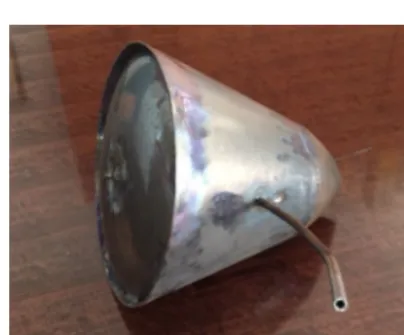
Figure 3.Proposed cone flowmeter.
4 Numerical simulations
In this paper, the evaluation of the features of both geome-tries has been primarily accomplished by means of a series of numerical simulations based on CFD (computational fluid dynamics) modelling. The target of the simulations is to es-tablish the extent of the influence of the inlet fluid flow rate and the influence of the cone diameter ratio β on the dis-charge coefficient and the improvements brought by the new geometry.
Figure 4.Piping system equipping the tested flowmeters.
4.1 Pre-analysis
The same strategy and criteria have been adopted for the nu-merical modelling of both systems. The simulation proce-dure is based on the solution of the governing equations, con-tinuum and momentum, with the adoption of an appropriate turbulence model aimed at providing the closure constraints to the RANS (Reynolds-averaged Navier–Stokes) equations. The RANS equations describe entirely the flow behaviour in steady and incompressible conditions. In this paper, the authors use the RNG (Re-Normalization Group) k– turbu-lence model (Markatos, 1986; Yakhot and Orszag, 1986). This model, coupled to an adequate near-wall treatment func-tion, describes efficiently the fluid motion for a wide range of industrial applications involving flow in pipes (Singh et al., 2009; Shah et al., 2012).
4.2 Governing equations and adopted mesh description The CFD provides the numerical solution of the governing equations of motion and describe the flow behaviour. The adopted mathematical model shall consider the flow general condition (incompressible or compressible) and the known boundary conditions.
The mathematical model is based on the mass, momen-tum, and energy conservation equations (for compressible flows). For incompressible flows, only the mass and momen-tum conservation equations are considered. In addition, for turbulent flows, the governing equations shall consider the velocity fluctuations around the mean value. In this case, the Reynolds decompositions of both flow pressure and veloc-ity allow us to give approximate time-averaged solutions to the governing equations (mainly mass and momentum for in-compressible flows).
In steady and incompressible conditions without any body forces, the time-averaged governing equations are provided in vector form.
∇ ·U=0 (2)
∇ ·(ρU·U)= −∇ ·P+ ∇ ·T (3)
Equation (2) is the time-averaged mass conservation, Eq. (3) the RANS. In Eq. (3), the termT is the overall stress tensor, provided by Eq. (4).
T =µeff[∇ ·U+(∇ ·U)T −2µeff∇ ·U I] (4)
In Eq. (4), the termµeffis the total effective dynamic
viscos-ity, provided by the following relation.
µeff=µ+µt=µ+ρ
Cµk2
(5)
In Eq. (5), the second term is a fictitious contribution due to the turbulence. The termCµis a constant. The introduc-tion of the Reynolds stresses in Eq. (4) requires two addi-tional transport equations for variables k and. The equa-tions are derived from the RANS equaequa-tions by means of the re-normalization group theory (Yakhot and Orszag, 1986).
Figure 6.Unstructured mesh for the S-G cone.
∇ ·(U·ρk)= ∇ ·[αkµeff∇ ·k]+Gk−ρ (6)
∇ ·(U·ρ)= ∇ ·[αµeff∇ ·]+C1
kGk+C2 2
k Gk
−ρ−R (7)
In Eq. (7), the term Gk is the generation of turbulent ki-netic energy due to the mean velocity gradient (Launder and Spalding, 1974), and it is calculated as Gk=µtS2. S is the mean rate of the shear stress tensor. The constants in Eqs. (6) and (7) are the standard values available in the liter-ature, according to Yakhot and Orszag (1986):Cµ=0.0845,
C1=1.42,C2 =1.68, andαk=α=0.7179.
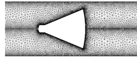
The governing equations are solved numerically using the finite-volume approach. According to this method, the entire geometric domain is divided into a finite number of cells. The flow simulations carried out for both geometries have been performed by means of the Ansys Fluent CFD com-mercial code (ANSYS, 2013). The principle of operation of the solver is based on cell-centred finite-volume approach. Therefore, an appropriate geometry discretization is crucial in order to get appropriate and accurate simulation results. Finer grids lead to more accurate flow evaluations, but they are computationally expensive. In the presented case studies, 2-D axisymmetric domains for both geometries are consid-ered along with an unstructured mesh of the flow domain. In order to get more refined and accurate results in the bound-ary layer of both pipe and flowmeter walls, an appropriate inflation strategy has been adopted.
Figure 6 shows the adopted mesh grid for the standard cone, and Fig. 7 illustrates the mesh of the proposed cone.
Figure 7.Unstructured mesh for the P-G cone flowmeter.
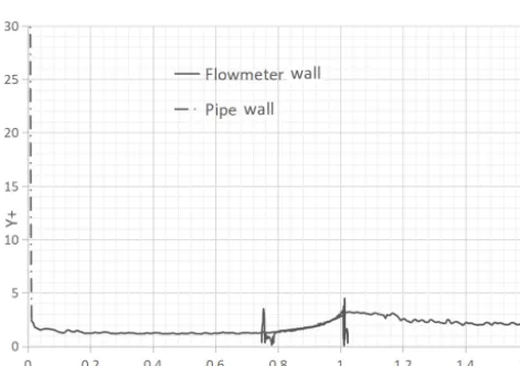
Figure 8. y+ trend in the flowmeter and pipe walls’ proximity, SG cone.
enhanced near-wall treatment functions in order to accurately resolve the flow condition in the boundary layer regions.
For both geometries, unstructured triangular meshes have been used in all the simulations. In the analysed cases, the unstructured meshing approach, adequately refined at the boundary layers, implies optimized setup time and computa-tional effort. In order to evaluate the suitability of the adopted meshing schemes, further attention has been dedicated to the analysis of the mesh goodness metrics. Checking the mesh quality plays an important role in the assessment of the sta-bility and the accuracy of the numerical computations. The most relevant goodness indicators are the orthogonal qual-ity, the aspect ratio (as a measure of the cell stretching), and the skewness of each cell (a measure of how closely ideal a cell is). The implemented mesh schemes are character-ized by cells with orthogonal quality and aspect ratios very close to 1 and a skewness never larger than 0.25. The solu-tion scheme implemented in the CFD solver is based on the pressure–velocity coupling using the SIMPLE scheme (AN-SYS, 2013). The gradients of pressure and velocity fields have been discretized according to the Green–Gauss node-based evaluation (which is claimed to be more stable for
Figure 9. y+ trend in the flowmeter and pipe walls’ proximity, PG cone.
triangle-based meshes). The adopted pressure interpolation strategy is based on the second-order scheme, and the spatial discretization of momentum, turbulent kinetic energy, and turbulent dissipation rate are based on the second-order up-wind scheme (ANSYS, 2013).
4.3 Boundary conditions
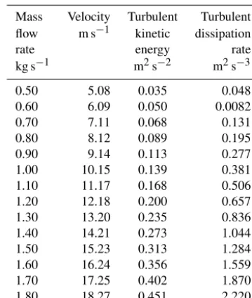
For all the simulations involving the two geometries, some specific boundary conditions have been set. The inlet mass flow rate (air at standard conditions) is among those condi-tions. Since the main purpose is to evaluate the discharge performance of both flowmeters, it has been considered an inlet mass flow rate ranging from 0.5 kg s−1up to 1.8 kg s−1 (corresponding to the operating flow range of the piping sys-tem). An operating relative pressure of 0 Pa has been set at the outlet and the no-slip condition for the walls has been considered. The first parameter to consider for a complete definition of the flow properties, at the inlet, is the turbulent intensity. For a fully developed flow, it can be estimated by means of Eq. (8) (Pope et al., 2000).
I=u 0
U =0.16(ReD)
1/8 (8)
In Eq. (8), the termu0 indicates the fluctuant velocity com-ponent andU the average component. According to the set inlet mass flow rate, the termI varies between 3 % and 4 %. The relationship between turbulent kinetic energy,k, and the turbulent intensity is
k=3
2(U I)
2. (9)
The turbulent dissipation rate is estimable from the turbulent length scale,l, according to Eq. (10).
=C
3 4
µ
k32
Table 1.Inlet boundary conditions for simulations relative to both cones.
Mass Velocity Turbulent Turbulent flow m s−1 kinetic dissipation
rate energy rate
kg s−1 m2s−2 m2s−3 0.50 5.08 0.035 0.048 0.60 6.09 0.050 0.0082 0.70 7.11 0.068 0.131 0.80 8.12 0.089 0.195 0.90 9.14 0.113 0.277 1.00 10.15 0.139 0.381 1.10 11.17 0.168 0.506 1.20 12.18 0.200 0.657 1.30 13.20 0.235 0.836 1.40 14.21 0.273 1.044 1.50 15.23 0.313 1.284 1.60 16.24 0.356 1.559 1.70 17.25 0.402 1.870 1.80 18.27 0.451 2.220
In Eq. (10), the terml is the turbulent length scale, which is 0.07Dfor fully developed flows in a pipe. The termCµis a constant (Launder and Spalding, 1974). The boundary con-ditions at the pipe inlet are summarized in Table 1.
4.4 Verification and validation of the CFD results The verification procedure determines whether the imple-mented mathematical model has been solved correctly. The task can be accomplished by checking the consistency of the obtained results with the mathematical model, the level of numerical errors (due to the discretization and linearization of the governing equations), and by means of a comparison with hand calculations (if those are easily available). The val-idation procedure, on the other hand, looks at whether the used mathematical model is correct and, therefore, consistent with the physical problem under study. The task is carried out by checking the simulation results against experimental data. In this paper, the verification procedure is performed through several steps. The preliminary and most basic step to imple-ment consists of a series of sanity checks on the pressure and velocity contours. The following step is a check whether the CFD solution honours the boundary conditions and the physical principles in the mathematical model (i.e. conser-vation of mass, momentum, and energy in the analysed do-main). The check of mass and momentum conservation in the whole domain is straightforward and, therefore, omitted in the paper. An appropriate subsection is dedicated to the energy balance. A further operation to perform (in the verifi-cation procedure framework) is the assessment of the accept-ability of the linearization error and the discretization error. The first is implemented by checking the residuals and the convergence rate of the solutions of governing equations. In
addition, a further check of the convergence rate of the drag coefficient is performed. The check of the discretization er-ror is performed by means of the comparison of the solutions obtained from the mesh refinement.
4.4.1 Energy balance check
For a steady incompressible flow, the energy conservation equation is provided by Eq. (11).
pin
ρ +
Uin2
2 =
pout
ρ +
Uout2
2 +lw (11)
Equation (11), valid for horizontal pipes, is the mechanical energy balance, in integral form, between inlet and outlet sections. The termlw represents the dissipation of energy, which is mainly due to viscous effects. For turbulent flows, the energy dissipation can be estimated by considering the turbulence characteristics, such as non-linearity, vorticity dif-fusivity, and dissipative attitude of the vortices at smaller scales. Indeed, the kinetic energy cascades down from larger to smaller eddy scales. At very smaller scales, the energy of eddies dissipates into heat, and such a phenomenon is due to viscous forces. The turbulent energy dissipation rate,, is the physical quantity for the estimation of the amount of energy lost by the viscous forces in the turbulent flow. Therefore, the termlwcan be estimated by means of Eq. (12).
˙ lw,=ρ
Z
dV (12)
Equation (12) is valid for incompressible flows, and it indi-cates the integral (over the whole flow domain) of the turbu-lent kinetic energy dissipation rate. In addition, the energy dissipation ratel˙w,B can be estimated by means of a time derivation of Eq. (11).
˙ lw,B= ˙m
1pL
ρ (13)
In Eqs. (12) and 13, l˙w,B is the time derivative of lw and
1pL is the permanent pressure loss between pipe inlet and
outlet. For turbulent incompressible flows, the energy bal-ance check can be performed by comparing the energy dissi-pation rate computed by means of Eqs. (12) and (13). In this subsection, the data of the energy balance check pertaining to some cases are reported, for brevity reasons.
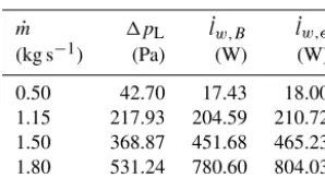
Table 2 shows the energy balance check for some simu-lations relative to the standard geometry cone. In all cases, there exists a significant agreement (within 3 %) between the energy dissipation rate computed by means of the Bernoulli equation,l˙w,B, and the dissipation rate computed by means of the volume integration of,l˙w,.
(kg s ) (Pa) (W) (W)
0.50 42.70 17.43 18.00 1.15 217.93 204.59 210.72 1.50 368.87 451.68 465.23 1.80 531.24 780.60 804.03
Table 3.Energy balance check for simulations relative to the pro-posed geometry cone.
˙
m 1pL l˙w,B lw,˙ (kg s−1) (Pa) (W) (W) 0.50 30.92 12.62 13.00 1.15 154.46 145.00 149.35 1.50 258.61 316.67 326.17 1.80 369.05 542.28 558.55
4.4.2 Mesh refinement analysis
The mesh refinement analysis allows us to check the level of discretization error.
Table 4 lists the number of elements and nodes relative to the computational grids of both flowmeters (considered as 2-D axisymmetric domains). In this section, for brevity rea-sons, only the comparison results relative to the simulations with an inlet mass flow rate of 1.8 kg s−1are considered.
Figure 10 shows the contour plot of the difference of the solutions of the axial velocity from the refined and original meshes for the standard cone. The contour plot is relative to the simulations with an inlet mass flow rate of 1.8 kg s−1. The maximum difference is about 3 %. Figure 11 shows the contour plot of the difference of pressures from both grids relative to the standard cone. For the pressure, the maximum difference is less than 1 %. The very limited difference of the velocity and pressure solutions obtained by a mesh refine-ment is a further step to the verification of the CFD tions. Analogous considerations are reported for the simula-tions carried out on the proposed cone flowmeter.
Figures 12 and 13 show the mesh refinement influence on the CFD results relative to the proposed geometry flowme-ter. In this case, the maximum discrepancy between the solu-tions of the axial velocity magnitude from both tested com-putational grids is about 3 %. For the pressure solutions, the maximum difference is about 0.5 %. Even for the simulations carried out on the proposed flowmeter geometry, the verifi-cation of the CFD simulations can be considered achieved.
The validation of the CFD simulations against experimen-tal data will be later discussed only for the proposed flowme-ter geometry, because experimental results could not have been obtained for the standard device due to the instability
S-G cone 100 306 225 691 Refined S-G cone 205 132 458 161 P-G cone 79 367 153 819 Refined P-G cone 140 004 273 456
Figure 10.Contour plot of the axial velocity difference between the original mesh and the refined one, S-G V-Cone.
of the flow caused by its unexpected fluctuation. Such a phe-nomenon has not occurred for the P-G cone, whose instal-lation is ensured by locking supports in the central area of the lateral surface of the cone at 180◦ from one another, as shown in Fig. 2.
4.5 Flow pattern analysis
Several simulations have been performed in order to evaluate the performance of the S-G cone with different inlet mass flow rates. In this section, only the solutions obtained with a flow rate of 1.8 kg s−1are considered.
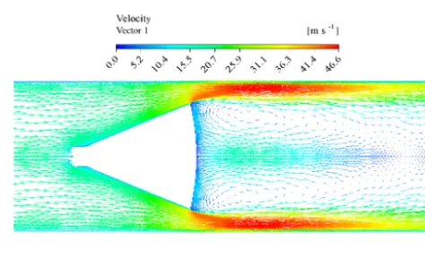
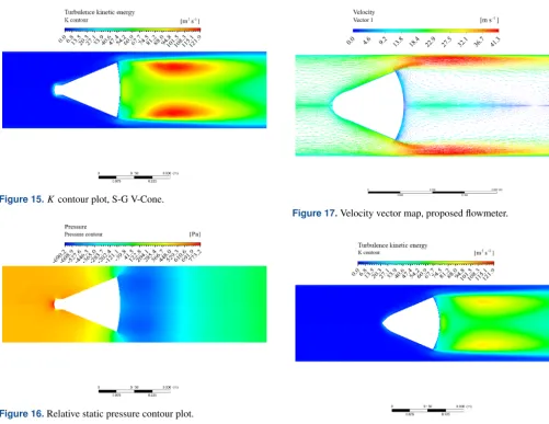
Figure 14 shows the velocity vector map. The flow is ap-proximately undisturbed upstream of the cone itself. Then, narrowing the cross section (due to the presence of the ob-stacle), the flow accelerates. The separation of the boundary layer on the rear side of the cone takes place, forming a free-flowing jet downstream. Turbulent wakes and recirculation regions can be observed just downstream from the flowme-ter. Figure 15 shows the turbulent kinetic energy contour plot. The largest values are located downstream, where the largest velocity gradients occur, due to the flow separation, and re-organized in recirculating zones.
max-Figure 11. Contour plot of the pressure difference between the original mesh and the refined one, S-G V-Cone.
Figure 12.Contour plot of the axial velocity difference between the original mesh and the refined one, proposed cone.
imum pressure drop, the decrease in flow kinetic energy causes an increase in the static pressure.
For the proposed cone geometry, the results of the simu-lations carried out with an inlet mass flow rate of 1.8 kg s−1 are going to be reported.
In this case, it is possible to make the same considerations relative to the standard cone. In addition, a comparison of Figs. 15 and 18 indicates that the amount of the turbulent ki-netic energy is dramatically reduced in the P-G cone. Indeed, the S-G geometry of the maximum value of the turbulent ki-netic energy iskMAX=121.8 J kg−1. For the P-G geometry,
kMAX=94.8 J kg−1, resulting in a reduction of the turbulent
kinetic energy of 13 %. Additionally, the extent of the dis-sipation rate of the turbulent kinetic energy is significantly reduced by 73 %.
Therefore, the introduced flowmeter geometry introduces fewer head losses (Eqs. 10, 12, and 13).
Figure 13.Contour plot of the pressure difference between the original mesh and the refined one, proposed cone.
Figure 14.Velocity vector map, S-G flowmeter.
The whole fluid flow pattern, through both flowmeters, has been analysed at different mass fluid flow rates, and, there-fore, at different Reynolds numbers. Figures 14 and 17 sug-gest that, for both cones, a pair of contra-rotating vortices in the recirculation zone, just downstream from the obstruc-tion, take place. The downstream extension of those vor-tices mainly depends on the obstruction geometry and the Reynolds number. At higher Re the axial extension of the downstream vortices increases. At anyRe, the proposed ge-ometry ensures slightly less extended recirculation zones.
Figure 20 shows the evolution of the velocity profile at different axial locations relative to the standard cone geom-etry. Figure 21 shows several velocity profiles (at the same locations as the S-G cone) observed in the proposed cone ge-ometry. In both cases, the recirculation region extends up to approximately 3-D, with an extended wake effect up to ap-proximately 5-D. Both figures refer to an inlet mass flow rate of 1.8 kg s−1.
Figure 15.Kcontour plot, S-G V-Cone.
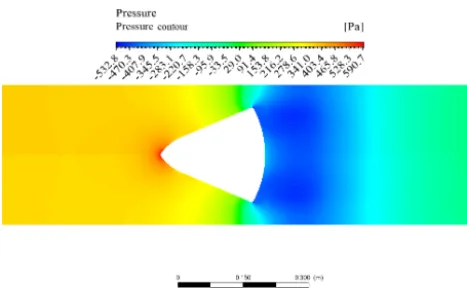
Figure 16.Relative static pressure contour plot.
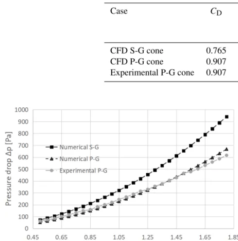
It can be noted that the proposed cone geometry ensures reduced pressure drops through the obstacle. Additionally, just upstream of both cones, the static pressure increases. In-deed, the presence of the obstruction within the pipe reduces the effective section. The converging section imposes a back pressure on the upstream, forcing the flow streamlines in the proximity of the pipe centreline to slow down and divert from the centre. The remarkable pressure drop, just downstream from the cone, is due to the flow acceleration through the an-nular section. Figure 22 suggests that for any mass fluid flow rate, the pressure drop experienced by the proposed cone ge-ometry is lower.
5 Results
In this section, the authors present a series of results about the evaluation of the performance ensured by the cones, with the purpose of pointing out the enhancements provided by the improved geometry.
Figure 17.Velocity vector map, proposed flowmeter.
Figure 18.Kcontour plot, S-G V-Cone.
5.1 Discharge coefficient
The discharge coefficient has been calculated by means of Eq. (1) using the data obtained from the CFD simulations and the experimental tests (only available for the proposed cone).
Figure 19.Relative static pressure contour plot.
Figure 20.Velocity profiles at different axial positions, S-G cone.
are coherent with the those available in the literature (Singh et al., 2006, 2009; Shah et al., 2012; Zhang and Dong, 2009). Figures 25–27 illustrate the results of the linear least squares fit of the linearized version of Eq. (1), for the stan-dard cone and the proposed one (based on CFD and ex-perimental data) (Eq. 14). The 9 parameter is provided by Eq. (15).
˙
m=CD·9 (14)
9=ZEFαK
p
2ρ1p (15)
Table 5 lists the computed CD, along with the standard
and extended uncertainties, and the fit determination coeffi-cientR2(Figliola and Beasley, 2010).
It is possible to point out the excellent agreement of the values, computed from the CFD simulations, with an adopted linear model. Additionally, it is possible to deduce the ex-cellent degree of concordance between the CFD simulations performed on the proposed cone and the relative experimen-tal data. Further, in this study, the authors analyse the perfor-mance ensured by both flowmeters with the cone diameter ratio β. With this aim, additional CFD computations have
Figure 21.Velocity profiles at different axial positions, P-G cone.
Figure 22.Relative pressure along the axial direction.
(95 %) R
CFD S-G cone 0.765 0 0 1.00
CFD P-G cone 0.907 0 0 1.00
Experimental P-G cone 0.907 0.006 0.012 0.998
Figure 23.Pressure drop due to the cone for both geometries.
Figure 24.Cdcoefficient against inlet mass flow rate.
a larger operating range ofβ, where it is possible to infer the mass fluid flow rate, by means of Eq. (1).
Figure 30 shows the influence of the cone diameter ratio on the discharge coefficient at two different mass flow rates (0.5 and 1.8 kg s−1). First, it can be confirmed that the
dis-charge coefficient remains quite unaffected by the inlet mass flow rate (as the flow is globally turbulent).
In addition, theCDof the standard geometry is influenced
by theβ ratio (or, equivalently, by pipe diameter), and it in-creases up to the asymptotic value of 0.792. On the other hand, the proposed cone geometry exhibits aCDcoefficient
unaffected by β. The CD variability should discourage the
Figure 25.Least squares regression fit, S-G cone.
Figure 26.Least squares fit of CFD data, proposed cone.
use of the standard cone in applications characterized byβ
different from the calibration condition.
5.2 Permanent pressure loss analysis
Figure 27.Least squares fit of experimental data, P-G cone.
Figure 28.Mach number contour map, S-G V-Cone,β≈0.620.
effect at the wall) because of the turbulent kinetic energy dissipation occurring just beyond the flowmeter, as has been pointed out in the energy balance check section.
Figure 31 illustrates the permanent pressure losses, for both cones, in the operating mass flow rate range, withβ=
0.726. The proposed geometry ensures less permanent pres-sure drops, as has been pointed out in the energy balance check section (Tables 2 and 3). In addition, it can be ob-served that the increase in1pLis of the same magnitude as
of1pthrough the cone, making their ratio constant with the flow rate. Figure 32 reports the permanent pressure losses, at two different mass flow rates, against the cone diameter ratio. It can be pointed out that the fluid dynamic losses decrease withβ. Indeed, the relative increase in pipe cross section in the cone insertion region decreases the effects of flow ac-celeration and pressure drop, resulting in less fluid dynamic losses. In addition, asβ increases, the downstream flow dif-fusion is more efficient, resulting in more limited permanent pressure losses.
6 Conclusions
The aim of the presented paper is to introduce a cone flowme-ter characflowme-terized by an optimized geometry. In order to assess
Figure 29.Mach number contour map, P-G V-Cone,β≈0.533.
Figure 30.Discharge coefficient vs.β.
Figure 31.Permanent pressure loss percentage against mass flow rate for both cones,β=0.726.
Figure 32.Permanent pressure loss percentage againstβfor both cones.
1. The proposed geometry introduces less downstream tur-bulence. Consequently, the turbulent dissipation rate, granted by the modified geometry, is more favourable. Such a behaviour implies less permanent pressure loss and a prompter static pressure recovery downstream.
2. The presented V-Cone exhibits fewer pressure drops, between the measuring pressure taps, for any tested mass flow rate (Fig. 23).
4. The discharge coefficient, ensured by the introduced ge-ometry, is 15.7 % larger for the tested conditions char-acterized by a cone diameter ratio of 0.726 (Figs. 24 and 30).
5. The influence of cone diameter ratio on the discharge coefficient has been analysed. The standard geometry exhibits a decreasing trend, asβ approaches lower val-ues. However, the proposed cone performance is un-affected by any variation of β in the studied range (Fig. 30), with no need for recalibration in case of cone insertion in a pipe with a different inner diameter.
6. The introduced flowmeter ensures less permanent pres-sure drops, due to the lower turbulence induced by the characteristic geometry.
Appendix A: Nomenclature
Symbol Description (physical unit)
˙
m Mass flow rate (kg s−1)
Cd Discharge coefficient
D Pipe inner diameter (m)
d Cone flowmeter base diameter (m)
ρ Fluid density (kg m−3)
1p Pressure drop through the cone flowmeter (Pa)
1pL Permanent pressure loss (Pa)
µ Molecular dynamic viscosity (Pa s−1)
β Cone diameter ratio
K Flow geometric coefficient
E Flow compressibility factor
Fα Material thermal expansion factor
u=U+u0 Reynolds decomposition of flow velocity vector
p=P +p0 Reynolds decomposition of flow pressure
k Turbulent kinetic energy (m2s−2) or (J kg−1)
Dissipation rate of turbulent kinetic energy (m2s−3) or (W kg−1)
r Radial coordinate
Competing interests. The authors declare that they have no con-flict of interest.
Acknowledgements. The authors would like to thank AC Boil-ers S.p.A. for the access to the data relative to the measurements performed on the test plant.
Review statement. This paper was edited by Rosario Morello and reviewed by two anonymous referees.
References
5167-5:2016: Measurement of fluid flow by means of pressure dif-ferential devices inserted in circular cross-section conduits run-ning full – Part 5: Cone meters, Standard, International Organi-zation for StandardiOrgani-zation, Geneva, CH, 2016.
ANSYS: ANSYS Fluent Theory Guide, ANSYS Inc., Canonsburg, PA, November 2013.
Borkar, K., Venugopal, A., and Prabhu, S.: Pressure measure-ment technique and installation effects on the performance of wafer cone design, Flow Meas. Instrum., 30, 52–59, https://doi.org/10.1016/j.flowmeasinst.2013.01.005, 2013. Figliola, R. and Beasley, D.: Theory and Design for Mechanical
Measurements, 5th Edn., Wiley, New York, 2010.
Hollingshead, C., Johnson, M., Barfuss, S., and Spall, R.: Discharge coefficient performance of Venturi, standard con-centric orifice plate, V-cone and wedge flow meters at low Reynolds numbers, J. Petrol. Sci. Eng., 78, 559–566, https://doi.org/10.1016/j.petrol.2011.08.008, 2011.
Ifft, S. A. and Mikkelsen, E. D.: Pipe elbow effects on the V-Cone flowmeter, Tech. rep., McCrometer, Hemet, CA, USA, 1993.
Appl. Math. Model., 10, 190–220, https://doi.org/10.1016/0307-904X(86)90045-4, 1986.
Miller, R.: Flow Measurement Engineering Handbook, Chemical engineering books, McGraw-Hill Education, New York, 1996. Pope, S., Pope, S., Eccles, P., and Press, C. U.: Turbulent Flows,
Cambridge University Press, Cambridge, 2000.
Prabu, S., Mascomani, R., Balakrishnan, K., and Konnur, M.: Effects of upstream pipe fittings on the performance of ori-fice and conical flowmeters, Flow Meas. Instrum., 7, 49–54, https://doi.org/10.1016/0955-5986(96)00001-5, 1996.
Sapra, M., Bajaj, M., Kundu, S., and Sharma, B.: Exper-imental and CFD investigation of 100 mm size cone flow elements, Flow Meas. Instrum., 22, 469–474, https://doi.org/10.1016/j.flowmeasinst.2011.07.002, 2011. Shah, M. S., Joshi, J. B., Kalsi, A. S., Prasad, C., and
Shukla, D. S.: Analysis of flow through an orifice me-ter: CFD simulation, Chem. Eng. Sci., 71, 300–309, https://doi.org/10.1016/j.ces.2011.11.022, 2012.
Singh, R., Singh, S., and Seshadri, V.: Study on the effect of ver-tex angle and upstream swirl on the performance characteristics of cone flowmeter using CFD, Flow Meas. Instrum., 20, 69–74, https://doi.org/10.1016/j.flowmeasinst.2008.12.003, 2009. Singh, S., Seshadri, V., Singh, R., and Gawhade, R.: Effect of
upstream flow disturbances on the performance characteristics of a V-cone flowmeter, Flow Meas. Instrum., 17, 291–297, https://doi.org/10.1016/j.flowmeasinst.2006.08.003, 2006. Yakhot, V. and Orszag, S. A.: Renormalization group analysis
of turbulence. I. Basic theory, J. Scient. Comput., 1, 3–51, https://doi.org/10.1007/BF01061452, 1986.