http://www.sciencepublishinggroup.com/j/ajmie doi: 10.11648/j.ajmie.20170204.13
Dynamic Analysis of Flexible-Link Planar Parallel
Manipulator with Platform Rigidity Considerations
K. V. Varalakshmi, J. Srinivas
*Department of Mechanical Engineering, NIT Rourkela, Rourkela, India
Email address:
[email protected] (K. V. Varalakshmi), [email protected] (J. Srinivas) *
Corresponding author
To cite this article:
K. V. Varalakshmi, J. Srinivas. Dynamic Analysis of Flexible-Link Planar Parallel Manipulator with Platform Rigidity Considerations.
American Journal of Mechanical and Industrial Engineering. Vol. 2, No. 4, 2017, pp. 174-188. doi: 10.11648/j.ajmie.20170204.13 Received: October 31, 2016; Accepted: May 13, 2017; Published: July 6, 2017
Abstract:
This paper presents dynamic analysis studies of planar parallel flexible 3-RRR manipulator with and without considering the flexibility of mobile platform. Initially, by treating all the members of the manipulator as flexible, the joint displacements, reaction forces and stresses are obtained during a specified trajectory tracking in Cartesian space. A comparative study is conducted with manipulator configuration having rigid mobile platform using coupled dynamics of limbs and kinematic constraints of mobile platform. Dynamic response of flexible manipulator is validated using ANSYS simulations for two different cases of trajectories. The results show a remarkable effect of flexibility of mobile platform on the overall dynamic response. After validation of the model, the inverse dynamic analysis data is used to create the system dynamics by employing generalized regression neural network (GRNN) model and the forward dynamic solutions of the flexible manipulator are predicted instantaneously. This study is useful for the real time implementation of motion control of flexible manipulators with complex dynamic model of manipulators.Keywords:
Flexible Manipulator, Static Analysis, Dynamic Modeling, Finite Element Method, Kinematic Constraints, Neural Network Model1. Introduction
In industrial environments, flexibility of links affects significantly the overall precision and performance and therefore it is of paramount importance in overall design. In certain applications like cable-driven manipulators or space robots where the links are of flexible type, a special design is adopted. In such cases, a single link can be defined as an assemblage of members connected to each other, such that no relative motion can occur among them. On the other hand, flexible manipulators offer several advantages such as higher speed, better energy efficiency, improved mobility and higher payload-to-arm weight ratio. At high operational speeds, inertial forces of moving components become quite large, leading to considerable deformation in the flexible links, generating unwanted vibrations [1-3]. It is therefore challenging task to achieve a high accuracy end-effector motion in flexible manipulators due to unwanted structural vibrations. Hence, elastic vibrations of lightweight links must be considered in the design and control of the manipulators
with link flexibility.
characteristics. Du et al. [18] discussed a method for the dynamic stress analysis of planar parallel robots with flexible links and a rigid moving platform and proposed a finite element-based dynamic model of flexible parallel robots. Zhaocai et al. [19] described a finite element method for dynamic modeling of parallel robots with flexible links and rigid moving platform. The elastic displacements of flexible links are investigated by considering the coupling effects between links due to the structural flexibility. Hu and Zhang [20] presented a method for the dynamic modeling of parallel robots with flexible links and rigid platform. Using constraint relations, the dynamic equations of the flexible links and rigid platform were obtained. The displacement and orientation errors of the moving platform were analyzed with numerical simulations. Shan-Zeng [21] derived the dynamic modeling equations of a 3-RRS manipulator with flexible links, analyzed the dynamic response of the end-effector, and indentified the actuator torques required to drive the flexible mechanism. Vakil et al. [22] introduced a method by combining the assumed mode shape approach and Lagrange’s equations to obtain a closed-form finite dimensional dynamic model for planar flexible-link, flexible-joint manipulators. Reis and Sada Costa [23] proposed a linear quadratic regulator theory for trajectory control of single link flexible arm. The vibration control of the manipulator was combined with piezoelectric actuation to improve the performance of the manipulator under parameter uncertainty. The dynamic characteristics of planar 3-RRR parallel manipulator with flexible linkages under temperature change are studies in [24-28] to determine the change of stresses in the links. Chen et al. [29, 30] developed a curvature-based finite element method for discretization of the flexible links for the dynamic modelling approach. They also proposed an approach for rigid-body motion and flexible-body motion. Zhao et al. [31] presented the kineto-elasto dynamic model and analyzed the dynamic characteristics related to natural frequency, sensitivity, energy ratios and displacement responses for the 8-PSS flexible redundant parallel manipulator. Dynamic analysis of parallel manipulators with link flexibility is one of the recent topics of research. In parallel manipulators, the mobile platform should be rigid enough to hold a cutting tool or welding torch. However, if other links have finite flexibility, the overall effect on motion and force control needs special attention.
In the present work, static and dynamic analysis of first kind of parallel manipulator namely planar 3-RRR manipulator with flexible links is considered. The kinematics including inverse analysis and Jacobian formulation are employed as subroutines for conventional rigid body dynamics. The presented two dimensional finite element formulation models the link flexibility of all limbs. After, formulating stiffness, inertia and nonlinear terms, the eigenvalue solutions are obtained for the cases with and without platform elasticity considerations. The remainder of paper is organized in the following: section 2 presents detailed description of dynamic model of flexible manipulators. Section-3 gives the kinematic constraints required in coupling rigid platform dynamics with
flexible limbs. The effect of platform rigidity on dynamic behavior is illustrated using two trajectory cases.
2. Dynamic Modeling
2.1. Description of Manipulator
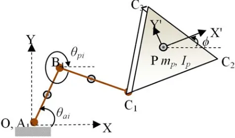
Dynamics of parallel manipulators has been studied over several years, but most of these are closed-form dynamic formulations compatible with rigid links. The 3-RRR (in which the underscore at first R indicates active revolute joint) manipulator considered here is a symmetrical three limb configuration planar parallel manipulator possessing three degrees of freedom (two translations and one rotation) at the mobile platform. Each limb is attached to fixed base platform with an active revolute joint. Figure 1 shows the line diagram of one of the limb in 3-RRR planar parallel manipulator.
Figure 1. Kinematic structure of 3-RRR Planar Parallel Manipulator.
2.2. Dynamic Analysis
The dynamic model of open-loop system of the 3-RRR mechanism can be expressed as:
t
τ q q
q q q
q) + ( , ) + ( ) =
( C N
M ɺɺ ɺ ɺ (1)
Where
1 9 T
]
,
,
[
∈
ℜ
×=
q
aq
pq
mq
is the joint vector,T 3 2 1, , ]
[ a a a
a = θ θ θ
q is the active joint vector,
T 3 2
1, , ]
[ p p p
p = θ θ θ
q is the passive joint vector,
1 9 T
]
,
,
[
∈
ℜ
×=
p pφ
m
x
y
q
is the mobile coordinate vector.1 9 T
]
,
,
[
∈
ℜ
×=
τ
τ
F
pτ
t a p is the torque vector.Here,
τ
a=
[
τ
a1,
τ
a2,
τ
a3]
Tis the input joint torque vectorof active joints and
τ
p=
[
τ
p1,
τ
p2,
τ
p3]
T=
[
0
,
0
,
0
]
T isthe input torque vector of passive joints. Also,
T
]
,
,
[
x y z p=
f
f
m
F
is the applied wrench vector at theend-effector.
q q)ɺɺ
(
torque. The above dynamic model can be simplified by considering external disturbances at the active joints.
The loop closure constraints are considered using a Jacobian matrix. From D’Alembert’s principle and the principle of virtual work, the configuration space can be smoothly parameterized by the actuator joint vector qa.
t
a τ
τ =WT (2)
where
∂
∂
=
a
p
u
q
q
I
W
(3)is the Jacobian matrix.
By using the matrix W from the equation (3), the dynamic model of equation (1) can be transformed into the closed-loop kinematic structure as:
a
τ
q
q
q
q
q
q
)
+
(
,
)
+
(
)]
=
(
[
TN
C
M
W
ɺ
ɺ
ɺ
ɺ
(4)Thus, they are expressed in terms of active joint coordinates. The complete dynamics of the closed-loop mechanism can be written as:
a a a a a a
a
q
q
q
q
q
τ
q
)
+
(
,
)
+
(
)
=
(
C
N
M
⌢
ɺ
ɺ
⌢
ɺ
ɺ
⌢
(5) where MW W M= T⌢ CW W W M W
C= T ɺ + T
⌢
N W N= T
⌢
Accordingly, the active joint torques can be computed. The dynamic model of equation (5) satisfies the following properties:
Property 1:
M
⌢
is positive definite and symmetric.
Property 2: M C
⌢ ⌢
2
− is a skew-symmetric.
Based on above set of equations of motion, an inverse dynamic module is developed as a separate function, which takes the Cartesian space trajectory as input and computes the necessary joint torques for a rigid body manipulator. The same formulation is used with finite element approach for solving the flexible linkages.
Before the static and dynamic equations of the manipulator can be obtained, it is necessary to derive strain and kinetic energy expressions of the flexible elements.
Therefore, the element strain energy of the beam element can be derived as
(6)
where qb is nodal displacement vector of plate, E is elastic
modulus of material, I is the cross-sectional moment of inertia and the elemental stiffness matrix (ke,b) is
− − − − = e e e e e e e e e e e e e e,b l EI l EI l EI symmetric l EA l EI l EI l EI l EI l EI l EI l EI l EA l EA 4 6 12 0 0 2 6 0 4 6 12 0 6 12 0 0 0 0 2 3 2 2 3 2 3
k (7)
where le is the length of the elemental beam. Likewise, the
element inertia matrix needed in dynamic analysis of linkage is obtained from kinetic energy expression and is given as
me,b= ∫e
A
b bℓ
0
T
N
dx
N
ρ
.where Nb is the shape function matrix of the beam element
[32]. When the flexibility of the mobile platform is considered, the platform is to be treated as a member moving in a plane. The simplest option is treating it as an assemblage of linear triangular elements (constant strain triangle). As shown in Fig. 1, for each node, there are two degrees of freedom.
Likewise strain energy of the plate element is
p
p q
q ep
p
e, T ,
2 1
U = k (8)
where ke,p is the element stiffness matrix and qp is the nodal
displacement vector of plate which can be given as
dA
A
p
=
∫∫
B
DB
k
Te, (9)
Here, B is strain-displacement matrix D is stress-strain relation matrix. Likewise, the element inertia matrix for the plate is obtained from kinetic energy expression and is given as:
b
q q eb b
e, Tb , 2 1
p e p p e p
e, = t
∫
NTN dAm
ρ
where Np is the shape function matrix of the plate element.
The element matrices are first converted into global fixed reference frame using the transformation matrix defined in terms of the angular position of the link (ϕ) with respect to the global frame. The coordinate transformation matrix Ts is defined as:
−
−
=
1
0
0
0
0
0
0
cos
sin
0
0
0
0
sin
cos
0
0
0
0
0
0
1
0
0
0
0
0
0
cos
sin
0
0
0
0
sin
cos
ϕ
ϕ
ϕ
ϕ
ϕ
ϕ
ϕ
ϕ
sT
(10)The stiffness and mass matrices of each element are thus given as Ke=Ts
T
keTsand Me=Ts T
me Tsrespectively.For the
study of kinematics and statics of the flexible linkage, the joint displacements, reaction forces and stresses are obtained from the following equation:
F
Q
=
K
(11)where K is the global structural stiffness matrix, Q is the global displacement vector and F is the global force vector.
The dynamic modelling of the manipulator can be obtained through assembly of element matrices with a standard finite element procedure. With the nodal displacement vector
T
]
,
[
q
bq
pq
=
using strain energy Ue, kinetic energy Te and non-conservative forces Fe, the Lagrangian equation can be written as e e e e F dt d = ∂ ∂ + ∂ ∂ − ∂ ∂ q q q U T Tɺ (12)
Substituting the element strain and kinetic energies of the beam and plate into the Eq. (12) we get,
e e e e e e
eQ +C Q +K Q = F
M ɺɺ ɺ (13)
Where Ce are the elemental mass, stiffness and damping
matrices of the system, respectively, Qe is the generalized
coordinate vector in the global reference frame and
f e gc e e F, F,
F = + is the total external force vector [25]. Here, ) ( T 9 T T 8 2 T 7 T s
,gc =T H ϕɺ −H Rp e−H ϕɺɺ
e r
F (14)
p f
e F
F T
s
, =T (15)
where, dv o dv dv o b v b v b v N I H N H N H ⌢ T 9 8 T
7 =
∫
ρP , =∫
ρ , =∫
ρP (16) − = − = 0 1 1 0 , cos sin sin cos I R ⌢
ϕ
ϕ
ϕ
ϕ
p (17)
Here, Ts = Transformation matrix and me are
elemental mass matrices of beam me,b and plate m e,p , =
e
k Elemental stiffness matrices of beam ke,b and plate p
e, k
= p
R Planar transformation matrix =
ϕ Angle between global to local frame =
ρ Density of the material
= o
P Location of coordinate vector in local frame = [xy]T
=
er
Position of element in local frame = [xy]T=
I
⌢
Skew-symmetric matrix = gc e,F Gyroscopic and Coriolis force components
= f e,
F Generalized external force vector
= p
F External force vector
By assembling all the elements in the Eq. (13) according to the compatibility at the nodes, the equations of motion of planar 3-RRR manipulator is given as
F
= + +CQ KQ Q
Mɺɺ ɺ (18)
where M, C and K are the global mass, damping and stiffness matrices of the system, respectively, Q is the global coordinate vector in the global reference frame. Rayleigh damping has been considered for the C in Eq. (13), which is a combination of mass and stiffness matrices given as follows:
K
M
C
=
ϖ
1+
ϖ
2 (19)where
ϖ
1 is the mass damping coefficient andϖ
2 is thestiffness damping coefficient. The material of the mechanism considered in numerical studies is the aluminium 1060 alloy with
ϖ
1= 0.02,ϖ
2 =0.0032.3. Finite Element Modeling
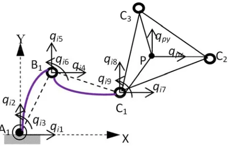
The deflected positions of the manipulator limb due to flexibility is shown in Figure 2. The design with a symmetric topology can achieve kinematic isotropy. The point P(xp, yp)T
is the end-effector position in the global reference frame and ϕ
Figure 2. Flexible 3-RRR Manipulator.
The point O is the origin of the fixed reference frame (not shown) and the points Ai, Bi, Ci, with i=1, 2, 3, define the
rotational articulations of each limb. qi is the elastic
displacement of links (i=1, 2, 3) and qpx and qpyare the elastic
displacements of the centre of the mobile platform. Points Ai
is actuated, so that all actuators are fixed to the base. Thus, the three fixed pivots A1, A2 and A3 define the geometry of a fixed base and the three moving pivots C1, C2 and C3 define the geometry of a moving platform. Together, the mechanism consists of eight links and nine revolute joints. The finite element formulation has been adopted here, which provides easier and systematic modeling techniques for complex mechanical systems and lays the groundwork for a general approach to the modeling of elastic mechanisms and manipulators. In order to verify and examine the dynamic performance of the 3-RRR flexible mechanism, the links in the mechanism are considered as a series of beam elements and the mobile platform as triangular plate element with flexible members undergoing flexural and axial deformations. In the present case, there are three degrees of freedom at each node, namely axial, transverse displacements and rotational angles. The mobile platform is considered as a constant strain triangle. It is divided into three elements; there are two degrees of freedom at each node, namely axial and transverse deflections.
3. Kinematic Constraints of a Rigid
Mobile Platform
When mobile platform is considered as rigid, its rigid body dynamics has to be added to the dynamics of flexible links with kinematic constraints. As shown in Figure 3, the center and vertices of the rigid mobile platform P and Cirespectively
are displaced to P' and Ci' due to elastic deformation of motion
of the flexible links. For rigid platform assumption the identity PCi = P'C'i is valid. To transfer the deformed vertices from
mobile frame to global frame, three transformation matrices
Tp1, Tp2, Tp3 for P-x-y to O-X-Y, P'-x'-y' to P-x-y and P'-x'-y' to O-X-Y respectively are considered, such that, Tp3 = Tp1Tp2.
Figure 3. Mobile platform configuration.
Also, if ∆Xp, ∆Yp, ζ are translational and rotational
displacements of the mobile platform due to elastic motion of the flexible links, the following expressions can be formulated. − = 1 0 0 Y cos sin X sin cos 1 p p
p φ φ
φ φ
T (20)
∆
∆
−
=
1
0
0
Y
1
X
1
2 p p pζ
ζ
T
(21)Assuming that (XCi, YCi) and (XC'i, YC'i) are the coordinates
of the points Ci and C'i in the global reference frame, we can
write ' ' C ' C 3 ' ' 1 1 Y X p i i p i C i C y x =
T (22)
p i i p i C y x = 1 1 Y X C C 1 i C
T (23)
where
(
,
)
(
',
')
C Ci i i
i
y
x
y
x
C C=
=(li3cos(
π
/2+2kπ
/3),li3sin(π
/2+2kπ
/3)for k=1, 2, 4.
If Qj, Qj+1, Qj+2 are the elastic displacements and elastic rotational angle at the end point Ci of the flexible link BiCi,
∆ ∆ = − = + ζ p p i i i C i i C i C j j y x Y X -R Y X Y X Q Q C C C ' ' 1
I (24)
∑ = +
=
19 , 12 ,5
Q
2j j
ζ
(25)where I is 2×2 unit matrix of the mobile platform. The equation of motion of a mobile platform in terms of local reference frame P-x-y is
p p pqɺɺ =F
M (26)
where = p p p p J m m
M is a diagonal matrix with mp
as the mass, Jp as the moment of inertia of mobile platform and
T ] , ,
[ px py pφ
p = q q q
q is the vector of deflections of the
mobile platform induced by the flexible deformation of the links and Fp is the vector of generalized external forces. Then,
the equation of motion of the mobile platform in terms of global reference frame O-X-Y is
p p p p p p
F
T 1 1 T1
M
T
Q
T
T
ɺ
ɺ
=
(27)Tp1 is the rotational transformation matrix, T
] , , [ p p φ
p = x y
Q is the deflection vector of the mobile
platform in global reference frame due to flexible link deformation. The kinematic constraints allow in assembling the equations of flexible links with that of mobile platform to obtain global equation of motion. If Eqs. (13) and (27) are expanded to system size and by incorporating damping, the equation of motion of the complete system can be expressed similar to Eq. (18).
3.1. Dynamic Characteristics and Sensitivity Studies
The free vibration problem is defined from the dynamic equations described earlier as follows:
0
)
(
−
ω
n2M
+
K
Θ
n=
(28)where Θn is the nth mode shape and the corresponding
natural frequencyωn. In order to obtain ωn the characteristic
determinant is equated to zero. i.e.,
0
)
det(
−
ω
n2M
+
K
=
(29)The effect of design parameters on the performance of the manipulator can be measured with sensitivity analysis. By taking the derivative of the frequency equation Eq. (26) with respect to the design parameter (namely the link lengths =
li1=li2=L)
0 )
(
2 2 2 =
∂ Θ ∂ + − + Θ ∂ ∂ + ∂ ∂ ∂ ∂ − L L L L n n n n n
n M K
K M
-M ω ω
ω
ω (30)
Taking dot product of Θnon both sides yields
0 ) (
2 2 T 2
T = ∂ Θ ∂ + − Θ + Θ ∂ ∂ + ∂ ∂ ∂ ∂ − Θ L L L L n n n n n n n
n M K
K M
-M ω ω
ω
ω (31)
Since,
{
(
)
}
0
)
(
2 2 TT
−
+
=
−
+
Θ
=
Θ
nω
nM
K
ω
nM
K
n (32)I
M
Θ
=
Θ
nT n (33)where I is the unit matrix. It can be simplified as
0
2
2 T TΘ
=
∂
∂
Θ
+
Θ
∂
∂
Θ
∂
∂
−
n n n n nn n
L
L
L
K
M
-
ω
ω
ω
(34)Therefore,
Θ
∂
∂
Θ
−
Θ
∂
∂
Θ
−
=
∂
∂
n n n n n n nL
L
L
K
M
T T 22
1
ω
ω
ω
(35)3.2. Generalized Regression Neural Network Model
Inspired from biological neural networks, artificial neural network (ANN) models can effectively predict the nonlinear
consists of an extra neuron compared to the output layer. This additional neuron calculates the probability density function, whereas remaining neurons are used for calculation of outputs. The GRNN chooses an approximate function which relates the input and the output parameters directly based on the training data. Thus, the GRNN is less time-consuming than other iterative training networks. As the forward dynamics is a difficult problem for flexible link mechanism, a neural network model is developed to approximate relationship between the joint torques and displacement, velocities. Figure 4 shows the GRNN architecture used for the dynamic studies.
Figure 4. Structure of GRNN Model.
GRNN finds joint probability density function of x and
y with a training set. The output from GRNN is estimated as
∑
−
∑
− =
= =
n
1
i 2
2 i n
1
i 2
2 i i
2 D exp
2 D exp Y ) X ( Yˆ
σ
σ (36)
where
(
X
i,
Y
i)
is a sample of(
X
,
Y
)
, D is the scalar 2ifunction and
σ
2is the squared bandwidth of the Gaussian RBF kernel given as:) X X ( ) X X (
D2i = − i T − i (37)
4. Results and Discussion
The static and dynamic performance of the 3-RRR flexible mechanism is verified with different positions of the following circular trajectory.
Circular trajectory:
sin(t) cos(t) × + =
× + =
r y y
r x x
p p
(38)
where r = 0.01m, t ∈ [0, 2π] and (xp, yp) = (0.25, 0.144).
Results are presented for static and eigenvalue analysis of
this manipulator with and without considering the flexibility of the mobile platform.
4.1. Static Analysis
In static analysis using inverse kinematic analysis the location of joints are identified to transform the mechanism from local to global frame. At the center of the platform a 10N force in X-direction is applied and with boundary conditions of the mechanism. The influence of flexibility at the mobile platform and elastic displacements at mobile platform along the trajectory are identified.
The material of the mechanism considered is the aluminum alloy Al-1060, the geometric and material properties are given in Table-1.
Table 1. Geometric and Material properties of linkage.
Parameter Dimension
Length of each link 0.2 (m)
Thickness of each link 0.0015 (m)
Width of each link 0.03 (m)
Length of the mobile platform 0.2 (m) Length of the base platform 0.5 (m)
Platform thickness 0.0015 (m)
Elastic modulus 6.9×10¹⁰ (N/m2)
Density 2700 (kg/m3)
Passions’ ratio 0.33
Mass of each link 0.0234 (kg)
Mass of the mobile platform 0.1205 (kg) Moment of inertia of the mobile platform 0.000799 (kgm2)
Moment of inertia of the links 0.00078 (kgm2)
As the user supplies the data, the program computes the global matrices and the equations are solved by inversion and resultant displacements (nodal data) and stresses (element data) are displayed at each point along the trajectory of the manipulator. Figure 5 shows the flowchart of the quasi-static approach, where a constant static load acts in every time-second.
Initially a set of trajectory points are specified and inverse kinematics is solved at each of these points. The global stiffness matrix in every posture is estimated. The active joint torques are obtained later using Jacobian matrix of rigid manipulator consideration and end-effector forces. The joint displacements are obtained as the solution of simultaneous algebraic equations formed from stiffness matrix and load vector Γ.
Case 1: All the links and mobile platform are flexible Figure 6 shows joint displacements at the active joints along the trajectory. The angular displacements at active joints are different and vary harmonically as the trajectory considered is circular and analysis is linear.
(a) Active joint A1
(b) Active joint A2
(c) Active joint A3
Figure 6. Active joint displacements.
Figure 7 shows the displacements at midpoint of the end-effector and it is observed that the displacement along X-axis is higher due to external force applied in that direction.
(a) X-displacements
(b) Y-displacements
Figure 7. Displacements at the end-effector point P.
Figure 8 shows the joint reaction forces in X and Y directions at active joints A1, A2 and A3 respectively obtained from element stiffness matrices.
(a) Reaction forces along X-axis
(c) Reaction forces along X-axis
(d) Reaction forces along Y-axis
(e) Reaction forces along X-axis
(f) Reaction forces along Y-axis Figure 8. Reaction forces at active joints.
These may be used to find the stresses in the links. In order to illustrate the effect of link flexibility on the kineto-static characteristics, the model is next analyzed in ADAMS (Automatic dynamic analysis of mechanical systems) software. The rigid body model of the mechanism is converted into a flexible one using model neutral file in ADAMS for the static force analysis. Figure 9 shows the meshed model in ADAMS with fully flexible links.
Figure 9. Meshed model in ADAMS.
To simulate the static displacements, a 10N force in X-direction is applied at the middle point of the mobile platform, the positions of the mechanism are specified by motion and the simulation is performed to know the joint displacements and reaction forces of the mechanism. Figure 10 shows joint displacements at the active joints.
(a) Active joint A1
(b) Active joint A2
(c) Active joint A3
Figure 11 shows the displacements at the midpoint of the end-effector and it is seen that the displacement magnitudes are well matched with the previously obtained beam element program results.
(a) Displacements along X-axis
(b) Displacements along Y-axis
Figure 11. Displacements at the end-effector point P.
The joint reaction forces in X and Y directions at active joints are illustrated at every point on the trajectory, which all well agreement with computer program results. From these results, it is observed that the static performance of the mechanism with the considered geometric parameters is moderate.
Case 2: Links are flexible and rigid mobile platform During transmission of motion, often the mobile platform is treated as a rigid member compared to the legs of the parallel mechanism. In such cases, the finite element meshing is applied to the legs and the motion transmission between different legs is achieved by kinematic constraint equations. In order to illustrate the rigid platform situation, the same circular trajectory is considered as in the previous studies. The joint displacements at the active are shown in Figure 12.
(a) Active joint A1
(b) Active joint A2
(c) Active joint A3
Figure 12. Angular motion at active joints.
Corresponding displacements (x, y and θ coordinates) at all the passive joints are also obtained. The corresponding displacements at the centre of the mobile platform are shown in Figure 13. It is seen that the displacements in X and Y directions of the mobile platform are relatively small in comparison with those of flexible mobile platform case.
(a) X-displacement
(b) Y-displacement
The joint reaction forces in X and Y directions at all the joints are computed. Here, the reaction forces at the active joints in X and Y directions are very much close to the earlier case of the flexible mobile platform.
Next, the simulation studies of rigid mobile platform with flexible links are carried out in ADAMS to find the joint displacements and reactions forces of the mechanism. The simulation is performed similar to previous study and the results obtained in post-processor are recorded. Displacements at the centre of mobile platform in X and Y directions are illustrated in Figure 14.
(a) Displacements along X-axis
(b) Displacements along Y-axis
Figure 14. Displacements at the end-effector point P.
4.2. Natural Frequency and Sensitivity Analysis
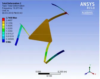
The theoretical model developed is used to compute the natural frequencies of the system with optimized dimensions, without considering motor dynamics and joint flexibilities. Modal analysis is conducted in ANSYS Workbench. The significance of natural frequencies is to assess the dynamic interaction between the links and its supporting structure. Design changes can also be evaluated by using natural frequencies and mode shapes of a structure. First few natural frequencies and corresponding mode shapes as obtained from ANSYS solution are shown in Figure 15.
(b) Second mode (16.973 Hz)
(c) Third mode (18.631 Hz)
Figure 15. First three mode shapes of the mechanism.
The results obtained from finite element analysis program developed in Matlab are compared with that of ANSYS outputs as shown in Table-2. It is observed that the first three modes are close to each other correspond to difference between the first to sixth natural frequencies is increasing from 6.86% to 37.46%.
Table 2. First six natural frequencies of the mechanism (Hz).
1 2 3 4 5 6
The sensitivity studies are carried out with respect to link lengths. Figure 16 shows the sensitivity distribution of first natural frequency within the workspace of the manipulator at orientations ϕ=0°, 10° and 30°. As all link lengths are considered the same, one case is only depicted.
(a) ϕ=0°
(b) ϕ=10°
(c) ϕ=30°
Figure 16. Sensitivities of the first order natural frequency to the link lengths.
When compared to the natural frequency, the effect of mobile platform orientation on sensitivity is more. As the orientation of mobile platform increases, the sensitivity also increases from 12.37% for ϕ=0° to ϕ=10° and 19.437% for
ϕ=0° to ϕ=30°. Due to flexibility in the linkage, sensitivity is more. Therefore, it is necessary to select optimum design parameters to improve the performance of the flexible planar parallel manipulator.
4.3. GRNN Model Implementation
The data obtained from inverse dynamics is used for the training, validation and testing of a neural network model approximating forward dynamics of the manipulator. A total of 631 points are considered in a circular trajectory and 379 of these data sets (60%) are used for training while remaining are used for validation.
The GRNN is implemented for the considered forward dynamic analysis is explained in the following steps.
Step 1: Initialize the 631 number of points data sets. Step 2: Among the 631 data points, consider first 60% of datasets for training the model.
Step 3: Obtain the smoothening parameter through cross validation procedure. In this analysis, grid search method is used to find the optimal adaptive parameter
σ
with minimum cross-validation error.Step 4: Determine the scalar function
D
i2(for i = 1–379) for ith node and determine the coefficient (exponential term) of Eq. (38) by substitutingD
i2andσ
2.Step 5: Multiply the calculated exponential term with the corresponding actual output data point Yi. This step is
processed in radial layer of the GRNN.
Step 6: For the obtained outputs of radial units, regression layer is used. The regression layer contains an extra neuron that calculates the probability density function of the output parameters.
Step 7: The weighted average of the GRNN output parameters are predicted in the observed range.
Step 8: To check the efficiency of the proposed method, the remaining 40% data sets are used for validating and testing.
Figures 17 and 18 show the actual joint displacements and velocities versus GRNN training data. The linear approximation is observed between the trained GRNN and experimental data with a minimal error.
Figure 17. Actual and predicted values of joint angles.
0 1 2 3 4 5 6
-0.7 -0.6 -0.5
Time (sec)
θa1
(
ra
d
)
0 1 2 3 4 5 6
1.4 1.5 1.6
Time (sec)
θa2
(
ra
d
)
0 1 2 3 4 5 6
-2.8 -2.6
Time (sec)
θa3
(
ra
d
) θa3 Actual θa3 Predicted
θa1 Actual θa1 Predicted
Figure 18. Actual and predicted values of joint velocities.
The graphical representation of the errors during GRNN training is depicted in Figure 19.
(a) Joint displacements
(b) Joint velocities
Figure 19. Graphical representation of errors.
A maximum of 0.05 error is found during GRNN training. The developed GRNN prediction tool was validated and compared with the actual data. Also, the proposed methodology is in good agreement with the
GRNN predicted and actual values. The proposed GRNN approach can be used to predict/calibrate the forward dynamics.
5. Conclusions
This work presented static analysis and dynamic coupling model for a flexible link planar 3-RRR parallel manipulator. Using finite element method the elastic displacements at the mobile platform due to the presence of flexible links in the mechanism was obtained. The numerical simulations are important in understanding the behavior of the flexible manipulator. The results show that the link flexibility has a significant effect on displacement errors in planar parallel manipulator. The modal frequencies of the fully flexible linear manipulator model have been validated with ANSYS solutions. Finally, the developed GRNN tool could predict the joint displacements and velocities within 0.05% error. The developed new tool efficiently predicts the relation between the input and output parameters. The work can be extended towards development of a trajectory controller that minimizes the flexibility effects.
References
[1] Z. Yang and JP Sadler, “On issues of elastic-rigid coupling in finite element modeling of high-speed machines,” Mech. Mach. Theory. vol. 35, pp. 71-82, 2000.
[2] A. Shabana, “Flexible multibody dynamics: review of past and recent developments.” Multibody Syst. Dyn. vol. 1, pp. 189– 222, 1997.
[3] Z. Zhou, J. Xi and C. K. Mechefske, “Modeling of a fully flexible 3PRS manipulator for vibration analysis”, J Mech. Des., Trans. ASME, vol. 128, pp. 403-412, 2005.
[4] B. Kang and J. K. Mills, “Dynamic modeling of structurally flexible planar parallel manipulator”, Robotica, vol. 20, pp. 329-339, 2002.
[5] X. Y. Wang and J. K. Mills, “FEM dynamic model for active vibration control of flexible linkages and its application to a planar parallel manipulator”, Appl. Acoust., vol. 66, pp. 1151-1161, 2005.
[6] P. K. Subrahmanyan and P. Seshu, “Dynamics of a flexible five bar manipulator”, Comput. Struct. Vol. 63, pp. 283-294, 1997. [7] E. Abedi, A. A. Nadooshan and S. Salehi, “Dynamic modeling
of tow flexible link manipulators”, World Academy of Sci., Eng and Technology, vol. 46, pp. 461-467, 2008.
[8] R. J. Theodore and A. Ghosal, “Comparison of the assumed modes and finite element models for flexible multilink manipulators”, Int. J. Robot. Res., vol. 14, pp. 91-111, 1995. [9] Z. Du and Y. Yu, “Differential motion equations of 5R flexible
parallel robot”, China Mech. Eng. Vol. 19, pp. 75-79, 2008. [10] M. Farid and W. I. Cleghorn, “Dynamic modeling of
multi-flexible-link planar manipulators using curvature-based finite element method”, J. Vib. Control. vol. 20 (11), pp. 1682-1696, 2014.
0 1 2 3 4 5 6
-0.1 0 0.1
Time (sec)
θad
1
(
ra
d
/s
e
c
)
0 1 2 3 4 5 6
-0.1 0 0.1
Time (sec)
θad
2
(
ra
d
/s
e
c
)
0 1 2 3 4 5 6
-0.1 0 0.1
Time (sec)
θad
3
(
ra
d
/s
e
c
)
θad1 Actual θad1 Predicted
θad2 Actual θad2 Predicted
θad3 Actual θad3 Predicted
0 1 2 3 4 5 6
-0.06 -0.04 -0.02 0 0.02 0.04
Time (sec)
J
o
in
t
d
is
p
la
c
e
m
e
n
t
E
rr
o
rs
(
ra
d
)
θa1 θa2 θa3
0 1 2 3 4 5 6
-0.05 0 0.05
Time (sec)
J
o
in
t
v
e
lo
c
it
y
e
rr
o
rs
(
ra
d
/s
e
c
) θ
[11] G. Piras, W. L. Cleghorn and J. K. Mills, “Dynamic finite-element analysis of a planar high-speed, high-precision parallel manipulator with flexible links”, Mech. Mach. Theory. vol. 40 (7), pp. 849–862, 2005.
[12] X. Wang and J. K. Mills, “Dynamic modeling of a flexible-link planar parallel platform using a substructuring approach”, Mech. Mach. Theory. vol. 41 (6), pp. 671–687, 2006.
[13] D. U. Zhao-cai and Y. U. Yue-qing, “Dynamic modeling and inverse dynamic analysis of flexible parallel robots”, Int. J. Adv. Robo. Syst. vol. 5 (1), pp. 115−122, 2008.
[14] S. K. Dwivedy and P. Eberhard, “Dynamic analysis of flexible manipulators: a literature review”, Mech. Mach. Theory. vol. 41 (7), pp. 749-777, 2006.
[15] X. Zhang, J. K. Mills and W. L. Cleghorn, “Dynamic modeling and experimental validation of a 3-PRR parallel manipulator with flexible intermediate links”, J. Intell. Robo. Syst.; vol. 50 (4), pp. 323-340, 2007.
[16] Y. L. Kuo, “Mathematical modeling and analysis of the Delta robot with flexible links”, Comput. Math. App. Vol. 71, pp. 1973–1989, 2016.
[17] B. Subudhi and A. S. Morris, “Dynamic modeling, simulation and control of a manipulator with flexible links and joints”, Robo. Auto. Syst. vol. 41 (4), pp. 257-270, 2002.
[18] T. Zhao, Y. Zhao, L. Shi and J. S. Dai, “Stiffness characteristics and kinematics analysis of parallel 3-DOF mechanism with flexible joints”, In: International Conference on Mechatronics and Automation; Harbin, China; 2007.
[19] Z. Du, Y. Yu and J. Yang, “Analysis of the dynamic stress of planar flexible-links parallel robots”, Front. Mech. Eng. China. vol. 2 (2), pp. 152–158, 2007.
[20] D. Zhaocai, Y. Yueqing and Z. Xuping, “Dynamic modeling of flexible-links planar parallel robots”, Front. Mech. Eng., vol. 3 (2), pp. 232–237, 2008.
[21] J. Hu and X. Zhang, “Dynamic modeling and analysis of a rigid-flexible planar parallel manipulator”, In: IEEE International Conference on Intelligent Computing and Intelligent Systems; Shanghai; 2009, DOI: 10.1109/ICICISYS.2009.5357817.
[22] S. Z. Liu, Y. Q. Yu, Z. C. Zhu, L. Y. Su and Q. B. Liu, “Dynamic modeling and analysis of 3-RRS parallel
manipulator with flexible links”. J. Cent. South Univ. Technol. vol. 17, pp. 323−331, 2010.
[23] M. Vakil, R. Fotouhi and P. N. Nikiforuk, “A new method for dynamic modeling of flexible-link flexible-joint manipulators”, J. Vib. Acoust. vol. 134 (1), pp. 014503–014503, 2011. [24] J. C. P. Reis and J. S. Costa, “Motion planning and actuator
specialization in the control of active-flexible link robots”, J. Sound Vib. vol. 331 (14), pp. 3255–3270, 2012.
[25] Q. H. Zhang, X. M. Zhang and J. L. Liang, “Dynamic analysis of planar 3-RRR flexible parallel robot”, In: Proceedings of the IEEE International Conference on Robotics and Biomimetics; Guangzhou, China; 2012.
[26] Q. Zhang and X. Zhang, “Dynamic analysis of planar 3-RRR flexible parallel robots under uniform temperature change”, J. Vib. Control vol. 21 (1), pp. 81–104, 2014.
[27] Q. H. Zhang and X. M. Zhang, “Dynamic modeling and analysis of planar 3-RRR flexible parallel robots”, J. Vib. Eng., vol. 26 (2), pp. 239–245, 2013.
[28] Hou W, Zhang X, Dynamic analysis of flexible linkage mechanisms under uniform temperature change. J. Sound Vib. 2009; 319: 570–592.
[29] Zhang Q, Fan X, Zhang X, Dynamic analysis of planar 3-RRR flexible parallel robots with dynamic stiffening. Shock and Vib. 2014; 1-13.
[30] C. Zhengsheng, K. Minxiu, L. Ming and Y. Wei, “Dynamic modelling and trajectory tracking of parallel manipulator with flexible link”, Int. J. Adv. Robo. Syst. Vol. 10 (328), pp. 1-9, 2013.
[31] Z. Chen, M. Kong, C. Ji and M. Liu, “An efficient dynamic modelling approach for high-speed planar parallel manipulator with flexible links”, Proc. Inst. Mech. Eng. Part C J. Mech. Eng. Sci. vol. 229 (4), pp. 663-678, 2014.
[32] Y. Zhao, F. Gao, X. Dong and X. Zhao, “Dynamics analysis and characteristics of the 8-PSS flexible redundant parallel manipulator”, Robo. Comp. Integ. Manuf, vol. 27, pp. 918–928, 2013.