http://www.sciencepublishinggroup.com/j/ijsda doi: 10.11648/j.ijsd.20170302.12
ISSN: 2472-3487 (Print); ISSN: 2472-3509 (Online)
Asymptotic Performance of the Location and Logistic
Classification Rules for Multivariate Binary Variables
Egbo Ikechukwu, Uwakwe Joy Ijeoma
Department of Mathematics, Alvan Ikoku Federal College of Education, Owerri, Nigeria
Email address:
[email protected] (E. Ikechukwu)
To cite this article:
Egbo Ikechukwu, Uwakwe Joy Ijeoma. Asymptotic Performance of the Location and Logistic Classification Rules for Multivariate Binary Variables. International Journal of Statistical Distributions and Applications. Vol. 3, No. 2, 2017, pp. 18-24.
doi: 10.11648/j.ijsd.20170302.12
Received: May 15, 2017; Accepted: May 24, 2017; Published: October 18, 2017
Abstract:
This paper focuses on the Asymptotic Classification Procedures in Two Group Discriminate Analysis with Multivariate Binary Variables. Two data patterns were simulated using the R-Software Statistical Analysis System 2.15.3 and was subjected to two linear classification namely; Location and Logistic Models. To judge the performance of these models, the apparent error rates for each procedure are obtained for different sample sizes. The results obtained show that the location model performed better than Logistic Discrimination with the variation in the error rates being higher for Logistic Discrimination rule.Keywords:
Apparent Error Rates, Location Model, Logistics Classification Rule, Multivariate and Binary Variable1. Introduction
Discrimination is a decision support tool with a wide range of applications, such as health applications, bankruptcy
prediction, education planning, taxonomy problems,
including engineering applications. It is a multivariate statistical classification technique for separating distinct sets of objects and allocating a new object to a previously defined group. In scientific literature, discriminant analysis has many synonyms such as classification, pattern recognition and character recognition, depending on the type of scientific area in which it is used. The technique usually proceeds in the following manner: a sample of objects is drawn from a population and partition of this sample is known. Each object within the population is described by several characters or certain measurements, which together form a feature vector belonging to a suitable feature space. Using the feature vectors and the individual labels of the sample, an allocation rule is established in order to classify other non-labeled objects from the previous population. The technique of discriminant analysis, though fairly old, still reflects inference in its applications. In attempting to choose an appropriate analytical technique, we sometimes encounter a problem that involves a categorical dependent variable and
several metric independent variables. If the dependent variable is metric, the undoubtedly multiple regression could be employed. A statistical technique that addresses the situation of a non-metric dependent variable is discriminant analysis. In this type of situation the researcher is interested in the predication and explanation of the relationship that affect the category in which an object is located, such as why a person is or is not a customer or if a firm will succeed or fail. The subject discriminant analysis has been well dealt with over the years. The review in the areas of logistic discrimination and the location model has been fairly presented in Krzanowski [1]. Some comparative studies on the location and logistic models have also been carried out with stringent data characteristics. The relative efficiency of these two statistical methods under different data conditions, however, has been an issue of debate (e.g Baron, [2], Dey & Austin, [3], Baah, [4]. A logical question is, how do the two techniques compare with each other? Research findings about the relative performance of the two methods appear to be inconsistent.
distributed with homogeneity of covariance, a linear discriminant function is used. A quadratic discriminant function is used if the covariances are not homogenous. The studies of Fan and Wang [5] and Lei and Koehly [6] made use of the assumption of normality. They considered the case of equal covariance and unequal covariance structures for the two groups.
Kakai, Pelz, and Palm [10] did a Monte Carlo study to assess the relative efficiency of the linear classification rule in 2, 3 and 5-group discriminant analysis. The simulation design took into account the number p of variables (4, 6, 10 and 18), the size sample n so that: n/p = 1.5, 2.5 and 5. Three values of the overlap, e of the populations were considered (0.05; 0.1; 0.15) and their common distribution was normal, chi-square with 12, 8 and 4 df; the heteroscedasticity degree, Γ was measured by the value of the power function of the homoscedasticity test related to Γ (0.05; 0.4; 0.6; 0.8). For each combination of these factors, the actual empirically computed error rate was used to calculate the relative error of the rule. The results showed that for normal or homoscedastic populations, the efficiency of the rule became better for large number of groups. Non-normality or heteroscedasticity negative impacted the performance of the rule whereas high values of the ratio n/p and high overlap have positive effect on the rule. The mean relative error of the rule became three
times more important from homoscedastic to
heteroscedasticity.
Bull and Donner [16] looked at the asymptotic relative estimated efficiency (ARE) of multiple LD compared with multiple DA. Two cases were considered – strong correlations between populations and no correlation between populations. In the first case, LD exhibited substantial increase in the ARE, while the second case exhibited no substantial increase in the ARE. It was also found that as the distance between populations increase the discriminant procedure does relatively better, with the logistic procedure eventually producing infinite parameter estimates when there is no overlap between populations.
Lei and Koehly, Egbo and Onyeagu, and Egbo [6, 8, 9], performed a Monte Carlo simulation to furnish information about the relative accuracy of Linear discriminant analysis
and logistic discriminant under various commonly
encountered and interacting conditions. The factors manipulated under multivariate normality are equality of covariance matrices, degree of group separation, sample size, and prior probabilities. They stated that the relative performance of the LDA and LD procedures depends on the interaction between model assumptions and population group distance. The degree of group separation was measured in terms of the squared Mahalanobis distance, ∆2 set at 2.68 (small and 6.7 (large). They found that if total misclassification is of interest, the optimal cut-score is 0.5. With a cut score of 0.5, LD and LDA with proportional or accurate prior specification perform similarly and best among other LDA specifications examined in the study, providing good to excellent classification accuracy for extreme population priors or large ∆2. In general they observed that
the misclassification rates were good for large ∆2.
In a study of Krzanowski [11], five different sets of data were used to evaluate the performance of Location Model with Fisher’s LDF, LD and a method in which all the continuous variables were converted to binary ones. The sample sizes considered for the data sets are as follows: a total of 40 – 20 from πI and 20 from π2; 63 from πI and 30
from π2; 38 from πI and 24 from π2; a total of 186 – 99 from
πI and 87 from π2; and a total of 137 – 59 from πI and 78
from π2; respectively for the data sets one to five. LM gave
satisfactory results and in the situation with relatively large sample size, gave much better results.
Efron [12] looked at the asymptotic relative efficiency of the normal discrimination procedure (LDA) and LD under multivariate normality, and found that this efficiency depends on ∆, the Mahalanobis distance between two normal populations, as well as on the number of individuals in each population. LD was shown to be between one-half and two-thirds as effective as LDA for statistically interesting values of the parameters. He stated that the LD procedures must be less efficient than the LDA at least asymptotically, as n ---> ∞. He further stated that though LD is less efficient and also more difficult to calculate, it is more robust, at least theoretically, than LDA.
Kakai and Pelz [10] performed a Monte Carlo study to assess the asymptotic error rate of linear, quadratic and logistic rules in 2, 3 and 5-group discriminant analyses. The simulation design that was considered took into account the overlap of the populations (e = 0.05, 0.1, 0.15), their common distribution (Normal, Chi-square with 12, 8 and 4 df) and their heteroscedasticity degree, Γ, measured by the value of the power function, 1 – βof the homoscedasticity test related to Γ (1 – β = 0.05, 0.4, 0.6, 0.8). For each combination of these factors, the asymptotic error of the 3 rules was computed using large samples of size 20,000. The efficiency parameter of the rules was their relative error with regard to the optimal error rate. The results showed the overall best performance of the quadratic rule for the normal heteroscedastic cases. The linear rule seemed to be more robust to an increased number of groups than the two other rules. The logistic rule was less affected by the distribution of the populations. For small size samples, the three rules become less efficient.
On the study of prior probabilities, Krzanowski [12] specified a range of values of p1 and p2 and 0.1 and 0.9 in a
Monte Carlo simulation to compare LM to Fisher’s LDF. He also varied the number of binary variables q between 2 and 4. It was observed that for equal priors, the error rates were a constant for both models. However, the error rates were found to decrease as p2 increased.
exceeds 1:3. For increased disproportional representation of the sample groups, the performance of the classification rule deteriorates, and its performance could not be improved by asymptotic increase in sample size.
The utility of an allocation rule can be assessed by the probabilities of misclassification or error rates, that it gives rise to. When parameters are known in the discriminant model the error rates are given by the optimum error rates, since they indicate the best results possible with the model. When parameters are unknown, various types of error rates may be distinguished. In particular, once an allocation rule has been derived in practice, it is essential to have a reliable method for estimating the error rates that it incurs to have some measure of its utility and to be able to assess its performance relative to other allocation rules. Accordingly, we need to consider methods of estimating the error rates arising from the allocation rule derived. Lachenbruch and Mickey [24], [7], [8], [9] discussed some means of estimating error rates for a given discriminant function. An object from π1may be misclassified into π2. Also an object from π2 may
be misclassified into π1. If misclassification occurs, a loss is
incurred. Let c (i/j) be the cost of misclassifying an object from πj into πi. The objective of the study is to find the best
classification rule. “Best here means the rule that minimizes the Expected Cost of Misclassification (ECM). Such a rule is referred to as the Optimal Classification Rule (OCR). In this study we want to find the OCR where X is discrete and to be more precise, Bernoulli.
2. Classification Procedures
2.1. Location Model
The classical discriminant analysis assumes that the discriminatory variable v is continuous and assumes normality. Often in practice, the discriminatory variable is a mixture of continuous and discrete variables. Let v denote a random vector of observations made on any individual which is a mixture of q discrete variables x and p continuous variables y. if the ith discrete variables has si categories (i =
1, …., q) then the contingency table formed from x has s = s1
x s2 x … x sq locations; and denote these locations by z1,
z2, …, zs. then the location model (LM) as proposed by
Krzanowski [14] has the following distribution assumptions: (1)The conditional distribution of y given that x falls in
location zm is
( ( , Σ
(2)The marginal distribution of the locations is given by
( = = , with ∑ = 1 (1)
Afifi and Elashoff [15] adopted the location model by allowing different values for the continuous variable location means µi(m)and multinomial probabilities pim (m = 1, …, s) in
the two populations (i = 1, 2) but constraining the conditional continuous variable dispersion matrix ∑ to be constant over all locations and over both populations. From the normality assumption of the model, the conditional probability density of y, given that the discrete variables locate the individual in cell m, is
( / | | − ( −
( ′Σ! ( − ( " (2)
In πi, (i = 1, 2). Thus the joint probability density of
obtaining the individual cell m and observing the continuous variable values y is
#$%
( / | | − ( −
( ′Σ! ( − ( " (3)
In πi, (i = 1, 2). Inserting these two joint probability
densities into the likelihood ratio rule, and tidying up the expression by algebraic manipulation yields the allocation rule:
Allocate the individual &′ = ( ′, ′) to πi if the discrete
variables x correspond to the mth multinomial cell and
( ( − ( )′*! − ( ( + ( )" ≥ ln (#% #%) (4)
Otherwise allocate v to π .
Given that the LM is appropriate, probabilities of misclassifications from populations π and π are shown to be.
= ∑0: 0Φ 23− ln 4 05 6 − △0 08 △5 90 (5)
= ∑0: 0Φ 23ln 4 05 6 − △0 08 △5 90 (6)
Where ∆j2 = (µ1(j)- µ2(j))∑-1 (µ1(j)- µ2(j)) is the Mahalanobis
squared distance between πI and π2 in cell j of the
multinomial table, and Φ(.) is the cumulative normal distribution function.
The allocation rule for the LM can be derived following basic principles. Define the conditional probability density of
y, the continuous variable, given that the discrete variable locate the individual in cell m, to be
; (< ∖ =
( >/ | | − ( −
( ′Σ! ( − ( " (7)
; (& = #$%
( >/ | | − ( −
( ′Σ! ( − ( " (8)
In πi, (i = 1, …, g). taking natural logs on both sides
?@; (& = ?@ − ?@A(2C D|∑|E − ( − ( ))′Σ! ( − ( )) (9)
= F + ?@ + ( ( ))′Σ! ( − ( )) (10)
Where q = - ½ ln((2Ӆ)c/∑/) – ½ y1∑-1y. Since q has the same value for all populations πi in cell m, the allocation rule
is
Allocate v1 = (yI, xI) to the population πi in cell m for
which
?@ + ( ( ))′Σ! ( − ( )) is greatest (11)
2.2. Logistic Discrimination
We have primarily concerned with discrimination and classification assuming a multivariate normal model for the variables in each group. However, one often finds that the variables in a study are not always continuous, but a mixture of categorical and continuous variables. If the group membership variable is categorical or a mixture with continuous, then logistic discrimination may be performed using logistic regression (Bull & Donner, [16]. “Logistic discrimination can be viewed as a partially parametric approach as it is only the ratios of the densities (fi(v)/fj(v), i ≠
j) that are being modelled.” (Mclachlan, [17]).
The logistic approach to discrimination is postulated as an alternative for discrimination and classification by parametric specification of the posterior probabilities P(π1/v) and P(π2/v)
where
(Π H⁄ ) = ORS (MJKL (MNOMPQ)
NOMPQ); (U H⁄ ) = ORS (MNOMPQ) (12)
With α0 = α0 – k, and k is any of the forms discussed
earlier. The fundamental assumption of the logistic approach to discrimination is that the log of the ratio of the group – conditional densities is linear, that is,
?@ V#(W Q#(W Q⁄ )⁄ )X = YZ+ Y[H. (13)
The classification rule, therefore is
if YZ+ Y[H ≥ 0, assign V to Π , (14)
Otherwise assign v to π2.
Directly generalizing the LD to the g-group case, the model for the posterior probabilities is given as:
(Π H⁄ ) = (YZ+ Y[H) (U^⁄ ) _ℎ a b1, … , dH ! (15)
(U^⁄ ) = H O∑e_ RS (MNOMPQ)
$g (16)
We therefore assign v to the group which has the greatest posterior probability. Thus
Allocate v to the population πi for which p(πi/v) is greatest.
2.3. Testing Adequacy of Discriminant Coefficient
Consider the discriminant problems between two multinomial populations with mean µ1 µ2and common matrix
∑. The coefficient of the MLD discriminant function a1x are given by α = ∑-1δ where δ= µ1µ2. In practice of course the
parameters are estimated by χi1 χi2 and S = m -1
{(n1 – 1)s1 + (n2
– 1)s2}, where m = n1 + n2 – 2
Letting the coefficient of the sample MLDF given by
j = k_! l
A test of hypothesis H0: αi = 0 using the sample
Mahalanobis distances D2p = Md1W-1d and D21 = Md1W11d
has been proposed by Rao (1965) this test statistics uses the statistic:
mn ! O oD (pq! pr)
( O D pq) s (17)
Where t = u uu under the null hypothesis has Fp – k, m –
p + 1 distribution and we reject H0 for large value of this
statistics.
2.4. Evaluation of Classification Function
One important way of judging the performance of any classification procedure is to calculate the error rates or misclassification probabilities (Richard and Dean, [18]). When the forms of parent populations are known completely, misclassification probabilities can be calculated with relative case. Because parent populations are rarely known, we shall concentrate on the error rates associated with the sample classification functions. One this classification function is constructed a measure of its performance in future sample is of interest. Total probability of misclassification (TPM) is given as:
v k = w ; l + w ; l x x (18)
The smallest value of this quantity by a judicious choice of R1 and R2 is called the optimum error rate (OER).
OER = minimum TPM
2.5. Probability of Misclassification
In constructing a procedure of classification, it is desired to minimize on the average the bad effects of misclassification (Onyeagu [19], Richard and Dean, [18], Oludare [20]). Suppose we have an item with response pattern x from either µ1 µ2. We think of an item as a point in a r-dimensional space.
We partition the space R into two regions R1and R2 which
as coming from µ1 and if it falls in R2 we classify it as coming
from µ2. In following a given classification procedure, the
researcher can make two kinds of errors in classification. If the item is actually from µ1the researcher can classify it as
coming from µ2. Also the researcher can classify an item
from µ2 as coming from µ1. We need to know the relative
undesirability of these two kinds of errors in classification. Let the priori probability that an observation comes from µ be q1, and from µ2 be q2. Let the probability mass function of µ1
be f1(x) and that of µ2 be f2(x). Let the regions of classifying
into µ1 be R1 and into µ2 be R2. Then the probability of
correctly classifying an observation that is actually from µ1
into µ1is
P(1/1) = ∑f1(x) and the probability of misclassifying such
an observation into µ2 is P(2/1) = ∑f1(x) similarly, the
probability of correctly classifying an observation from µ2 to µ2 is P(2/2) = ∑f2(x) and the probability of misclassifying an
item form µ1 into µ2 is P(1/2) = ∑f2(x)
The total probability of misclassification using the rule is
TPMC(R) = q1 ∑f1(x) + q2 ∑f2(x)
In order to determine the performance of a classification rule R in the classification of future items. We compute the total probability of misclassification known as the error rate. Lachenbruch [21] defined the following types of error rates.
(i)Error rate for the optimum classification rule, Ropt.
When the parameters of the distributions are known, the error rate is
TPMC (R) = q1 ∑f1(x) + q2 ∑f2(x) which is optimum for
this distribution.
(ii)Actual error rate: the error rate or the classification rule as it will perform in future samples.
(iii)Expected actual error rate: the expected error rates for classification rules based on samples of size n1 from π1
and n2 from π2.
(iv)The apparent error rate: this is defined as the fraction of items in the initial sample which is misclassified by the classification rule.
Table 1. Confusion matix of apparent error rate.
π1 π2
π1 n11 n12 n1
π2 n21 n22 n2
N
The table above is called the confusion matrix and the apparent error rate is given by
(yt) = @ + @@
Hills [22] called the second error rate the actual error rate and the third the expected actual error rate. Hills showed that the actual error rate is greater than the optimum error rate ad it in turn is greater than the expectation of the plug-in estimate of the error rate. Martin and Bradley [23] proved a
similar inequality. An algebraic expression for the exact bias of the apparent error rate of the sample multinomial discriminant rule was obtained by Goldstein and Wolf [24]. Who tabulated it under various combinations of the sample sizes n1 and n2. The number of multinomial cells and the cell
probabilities. Their results demonstrated that the bound described above is generally loose.
3. Simulation Experiments and Results
The two classification procedures are evaluated at each of the 118 configurations of n. r and d. the 118 configurations of n. r and d are all possible combinations of n = 40, 60, 80, 100, 200, 300, 400, 600, 700, 800, 900, 1000, r = 3, 4, 5 and d = 0.1, 0.2, 0.3 and 0.4. a simulation experiment which generates the data and evaluates the procedures is now described.
(i) A training data set of size n is generated via R – program where n1= n/2 observations are sampled from
π1. Which has multivariate Bernoulli distribution with
input parameter p1 and n2 = n/2 observations sampled
from π2 which is multivariate Bernoulli with input
parameter p2 j = 1 …. r. these samples are used to
construct the rule for each procedure and estimate the probability of misclassification for each procedure is obtained by the plug-in rule or the confusion matrix in the sense of the full multinomial.
(ii) The likelihood ratios are used to define classification rules. The plug-in estimates of error rates are determined for each of the classification rules. (iii)Step (i) and (ii) are repeated 1000 times and the mean
plug-in error and variance for the 1000 trials are recorded. The method of estimation used here is called the re-substitution method.
The following table contains a display of one of the results obtained
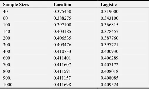
Table 2. Effect of input parameters P1 and P2 on classification rules at various values of sample size and Replications (mean apparent error rates).
Sample Sizes Location Logistic
40 0.375450 0.319000
60 0.388275 0.343100
100 0.397100 0.366815
140 0.403185 0.378457
200 0.406535 0.387760
300 0.409476 0.397721
400 0.410733 0.400930
600 0.411401 0.406289
700 0.411607 0.407172
800 0.411591 0.408018
900. 0.411157 0.408085
1000 0.411698 0.409524
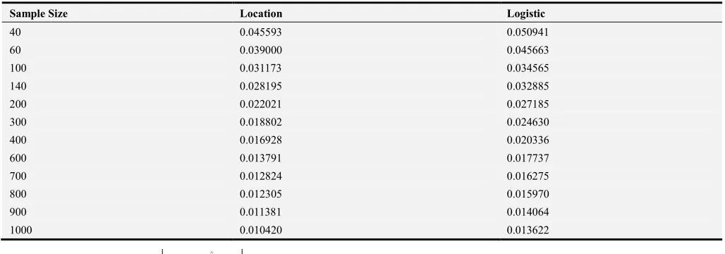
Table 3. Effect of input parameters P1 and P2 on classification rules at various values of sample size and Replications (actual error rates).
Sample Size Location Logistic
40 0.045593 0.050941
60 0.039000 0.045663
100 0.031173 0.034565
140 0.028195 0.032885
200 0.022021 0.027185
300 0.018802 0.024630
400 0.016928 0.020336
600 0.013791 0.017737
700 0.012824 0.016275
800 0.012305 0.015970
900 0.011381 0.014064
1000 0.010420 0.013622
P1 = (.3,.3,.3,.3), P2 = (.4,.4,.4,.4), ( ) ( ) ∧
−
p m c p m c
Table 4. Total Ranks for performance on 21 population pairs by the classification rules.
r = 3 r = 4 r = 5 Total Position
LM 1 1 1 1 1 1 1 1 1 1 1 1 1 1 1 2 2 2 2 2 2 27 1
LD 2 2 2 2 2 2 2 2 2 2 2 2 2 2 2 1 1 1 1 1 1 36 2
A glance in tables 1, 2, and 3 Mean apparent error rates increases with the increase in sample sizes in the two classification rules under study. The actual error rate decreases with the increase in the sample sizes. Location Model ranked first followed by Logistic Regression Model. The results presented in this paper have practical implications for the decision of when to use each technique. Because of its demonstrated high levels of accuracy, Location Model may be the method of choice when the researcher is most interested in recovering the highest percentage of correct classification. However, as the results of both studies indicate, there are times when Logistic Modeling may provide a better alternative. In situation where the numbers of variables are large, Logistic Modeling has demonstrated higher levels of classification accuracy.
4. Conclusions
In this study, there was a decline in the misclassification error rates for both location and logistic models as the sample size increases. The error rates of misclassification reduces rapidly as group separator increases. Logistic model showed higher coefficient of variation than location model in general.
The results from the present studies provide strong implications for the practical use of location and logistic models. Research into misclassification analysis is very important for understanding when to use which classification method and the implications of using one method over another. A better understanding of these concepts will eventually lead to better accuracy in classification and better accuracy in classification should be a goal for all areas of research that are classification methods.
Recommendations
Based on our findings we recommend as follows:
1 Location model should be used when it is necessary to increase the distance function and samples sizes.
2 Location model should be preferred over logistic model
for smaller number of variables.
References
[1] Krzanowski, W. J. (1988). Principles of Multivariate Analysis: Users perspective. New York: Oxford University Press. [2] Baron, A. E. (1991), Misclassification among methods used
for multiple group discrimination. The effects of distributional properties. Statistics and Medicine, 10, 757-766.
[3] Dey, E. l. & Austin, A. W. (1993). “Statistical alternatives for studying college student retention: A comparative analysis of logit, probit and linear regression”, Research in Higher Education, 34, 569-581.
[4] Baah, P (2012): comparative study of the logistic regression and the discriminant analysis journal of statistical computation and simulation 29 (2): 140 – 150.
[5] Fan, X., & Wang, L. (1999). Comparing linear discriminant function with logistic regression for the two-group classification problem. The Journal of Experimental Education, 76 (3), 265-286.
[6] Lei, P., & Koehly, L. M. (2003). Linear discriminant analysis versus logistic regression: A comparison of classification errors in the two-group case. Journal of Experimental Education, 72, 25-49.
[8] Egbo, I., Egbo, M. & Onyeagu, S. I. (2015). Performance of Robust Linear Classifier with Multivariate Binary Variables. Journal of Mathematics Research, Vol. 7, No. 4 Pp. 104-111. [9] Egbo, I., Onyeagu, S. I. & Ekezie, D. D. (2016). Derivation of
Extended Optimal classification rule for multivariable Binary variables. Journal of Theoretical mathematics and Applications, vol. 6 Issue 2.
[10] Kakai, R. L. C., Pelz, D., 7 Palm, R. (2010). On the efficiency of the linear classification rule in multi-group discriminant analysis. African Journal Of Mathematics And Computer Science Research, 3 (1), 19-25.
[11] Krzanowski, W. J. (1975). “Discrimination and classification using both binary and continuous variables”, Journal of the American Statistical Association, 70, 782-790.
[12] Efron, B. (1975). “The efficiency of Logistic Regression compared to Normal Discriminant Analysis. Journal of American Statistical Association 20, 892-898.
[13] Adebanji, A. O. (2008). Effect of sample size Ratio on the performance of the Linear Discriminant Function; International Journal of Modern Mathematics 3 (1), 97-108.
[14] Krzanowski, W. J. (1993). Location model for mixtures of categorical and continuous variables. www.Springer.com. article.
[15] Afifi, A. A., & Elashoff, R. M. (1969). Multivariate two samples test with dichotomous and continuous variables. i. the location model. The Annals of Mathematical Statistics, 40(1), 2990-298.
[16] Bull, S. B., & Donner, A. (1987). The efficiency of multinomial logistic regression compared with multiple group discriminant analysis. Journal of the American Statistical association, 82 (400), 1118-1122.
[17] McLachlan, R. (1992). Discriminant Analysis and Statistical Pattern Recognition. John Wiley and sons Inc., New York. [18] Richard, A. J., & Dean, W. W. (1998). Applied Multivariate
Statistical Analysis. 4th edition, Prentice Hall, Inc. New Jessey.
[19] Onyeagu, S. 1. (2003). Derivation of an optimal classification rule for discrete variables. Journal of Nigerian Statistical Association vol 4, 79-80.
[20] Oludare, S. (2011). Robust Linear classifier for equal Cost Ratios of misclassification, CBN Journal of Applied Statistics (2) (1).
[21] Lachenbruch, P. A. (1975). “Discriminant Analysis”. Hafrier press New York.
[22] Hills, M. (1967). “Discrimination and allocation with discrete data”, Applied Statistics, 16, 237-250.
[23] Bradley E. (1972). Improving the usual estimator of a normal covariance matrix. Department of Statistics Technical Report 37, Standard University.
[24] Goldstein & Wolf (1977). On the problem of Bias in multinomial classification. Biometrics 33, 325-331.