Published online February 20, 2014 (http://www.sciencepublishinggroup.com/j/ijepe) doi: 10.11648/j.ijepe.20140301.13
New solution method of wave problems from the turning
points
Kamal SheikhYounis
1, Nikolay Evgenevich Tsapenko
21Department of Electrical Engineering, Salahaddin University, Erbil, Iraq 2Department of Mathematics, Moscow State Mining University
Email address:
[email protected] (K. Younis), [email protected] (N. E. Tsapenko)
To cite this article:
Kamal SheikhYounis, Nikolay Evgenevich Tsapenko. New Solution Method of Wave Problems from the Turning Points. International Journal of Energy and Power Engineering. Vol. 3, No. 1, 2014, pp. 15-20. doi: 10.11648/j.ijepe.20140301.13
Abstract:
One of the main challenges in wave processes is the problem of eventuality correctness of different asymptotic representations of the same exact solution taken from different sides of the turning point. In this paper a universal solution method of this problem has been developed and the particular solutions of the wave equation have been expressed in terms of the solutions of Riccati’s equation for which the proper values in the turning points have been obtained. The paper demonstrates that, just those values will breed a correct phase and amplitude correlations in wave functions. Exact quantization conditions have been deduced and exact formulas for reflection and passage coefficients of quanta mechanical particles of potential barrier have been derived.Keywords:
Wave Problem, Riccatti’s Equation, Quantization Condition1. Preliminary General Correlations
Let in the interval (a, b) defines some differentiable function of complex value w = w(x).
Let u = u(x), v = v(x), are its real and imaginary parts respectively. Then
w=u+ iv, (1)
u= , v= . (2)
We introduce the logarithmic derivatives of those functions
q= i ,γ1= ,γ2= . (3)
Assuming that in a fixed point x0 (a,b)
w(x0) = A0 ei , u(xo) = A1, v(x0) = A2,
So the reverse equality to the equality (3) would be w = A0e ° , u = A1 e ,
v = A2e ° , (4)
Where four constants A0,φ , A1,A2 , are affiliated by
conditions
A1=A0cosφ , A2=A0sinφ0. (5)
Now we find the correlations associating q, γ!,and γ .
Differentiating expressions (1), (2) and substituting them in (3) we obtain
q=I " # $
! #$ , (6)
γ!% i
& &
! && , (7)
γ = i &&
! && , (8)
And as a consequence of the later two equalities, the following equality can be obtained
q=i{ + } (9)
Assuming that, φ = argw, ρ % │q │, θ = arg q, We device the relations (7),(8) to the following shape
γ!=ρ) * +./) ,-,γ =ρ./) +) * ,- (10)
Then
Based on the later equality, it is not difficult to conclude, that the function ρ (x) is always located between functions
γ!2(x) and γ 2(x).It means that it always implements one of
the inequalities, either
γ!20 ρ 0γ 2, or γ 20ρ 0γ! 2 .
Assume, that functions γ!+x-and γ +x- are determined,
such that in the point x0 (a,b) they satisfy the condition γ!(x0)=γ (x0)=γ >0. (12)
Hence, undoubtedly in this point results
ρ(x0)=γ (13)
Putting (12), (13) in (10) we come to agreement, that the values of arguments φ0 = φ (x0),
Θ0 = θ (x0) have to be connected as
φ0+ =34 (14)
Emphasizing, once again this important result for the theory of wave equation: from condition (12) yields condition (14) and vice versa, if (14) is implemented, so (12) would implement too.
2. Representation of Precise Solution
Consider functions w(x), u(x), v(x) mentioned in the previous paragraph are certain particular solutions of wave equation of
5″+
6+7-8 5=0 (15)
With smooth real coefficient r(x), small positive parameter 9 and with one turning point of the first order (r(x0) = 0, but r′(x0) : 0).
In this case the logarithmic derivative of (3) should be the solution of the corresponding Riccati equations. Thus
;′=i<
6+7-8 ; =, (16) >′=
6+7-8 +>! (17)
>′=
6+7-8 > . (18)
Recasting those equations in the form of
iq= ??′+@<; A6+7-8 ?!=, (19)
>!= B
′
B !{>
!–6+7-8 B!} (20)
> = BB′ +!<> 6+7-8 B!= (21)
Expressing
P=!<; A6+7-8 !?=, (22)
D!=!<>! 6+7-8 B!=, (23)
D =!<> 6+7-8 B!=. (24)
In a region, where r(x) >0 at 9 E 0, we arrive to asymptotic equalities
q=F6+7-8 +(1+o(9--,p=F6+7-8 ((1+o(9 )). (25)
In an area, where r(x) < 0 at 9 E 0 we obtain
>!=F 6+7-8 +1 A H+9--,D!=F 6+7-8 +1 A H+9 --, (26)
> =F 6+7-8 (1+O(9--,D =F 6+7-8 (1+O(9 --. (27)
Assume, that in the turning point x = I the solutions of equations (16) – (18) will have these values
q(I )=> JKL ,>
! +7 -=>+7 -=> , (28)
That is to say, satisfy conditions (12), (13). Furthermore integrating the left and right hand sides of the equations
(19) – (21), we obtain
i 77 ;MI=!lnB?+iL+i77 NMI, (29)
>77 !dx=!lnBB 77D! dx, (30)
> 7
7 dx=!lnBB + D
7
7 dx. (31)
Inserting those presented integrals of precise solution of Riccati equation into the three exact particular solutions of the wave equation, which is mentioned in (4).
In formula (4) taking the conditions (5) and (14) into account and assigning the multiplication
F> A0 as a new arbitrary constant C0. We obtain
w=O
√?J
@<Q R UUST7=, (32)
u=O VWXY
√? J
Z[U
U
U (33)
v=O X@\Y
√B J
Z T7
U
U . (34)
Now, we determine the argument ] , on the basic of the well-known semi classical amplitude correlations for main members of standard asymptotic expansions solution of wave equation.
By moving from turning point in the region of positive values of the coefficient r(x), the main member of asymptotic notation of precise solution (32) can be written as
^_=RO√6J@< Q
R ` UU√6T7 =. (35)
solutions (33), (34) are obtained from the main member of (35), and according to the initial definition of the functions u and v as the real and imaginary parts of the function w. Therefore,
ab=RO√6cde <f 4A! 8 77√g MI=, (36)
hb=RO√6eij <f4A8 ! 77√g MI=. (37)
When moving from turning point in the region of negative values of the coefficient r(x), the main members of asymptotic notations precise solutions (33), (34) will be as follows
ab=O VWXYR√ 6 J ` √ 6T7
U
U , (38)
hb=OR√ 6X@\Y J` √ 6 T7
U
U . (39)
Further, follows that we have to distinguish two cases, when in the turning point
g′+I ) <0, and when g′+I - >0.
1. Let the turning point g′(I ) <0. Then according to
the semi classic functions, the expressions (36) and (38) would be the main members of the asymptotic representation of the one and the same precise solution of the wave equation, only if their amplitudes satisfy the condition
O
=k cos] . (40)
Hence, we obtain the value of the argument ] ,
] =fl (41) And from condition (14) we find that, in the turning point, in which g′+I
- < 0 the argument value of precise
solution of Riccati equation (16) should be certainly as follows
m = fn! (42) Substituting the value (41) in (39), we obtain the main member of asymptotic expansion of the precise growing exponential solution which cannot be obtained using traditional phase integral method.
2. Let in the turning point g′(x
0) > 0. Then functions
(37) and (39) will be semi classical approximate of the one and the same precise solution of the wave equation, only if their amplitudes satisfy a condition
O =k sin] (43)
Hence, we obtain the value of argument ]
] =fn (44) And from condition (14) we find that, in the turning point, in which g′(I ) > 0 the argument value of precise
solution of Riccati equation (16) should be necessarily as follows
m =fn! (45)
Substituting (44) in (38), we obtain the main member of asymptotic expansion of the precise growing exponential solution of wave equation.
So, in this point a new important result has been obtained, opening an easy approach for the problem solution of wave propagation with turning point in a heterogeneous medium .This method is absolutely analogous with a standard method based on the sewing solution on the medium parts’ boundaries with different wave parameters. Now we are in a position to summarize the result.
The solution of the wave equation (15) with the turning point should be constructed in a form of linear combination of particular solutions where, in region r(x) > 0 is in a form of linear combination of function types
J@ ?T7 ,J ? T7 ,
And in a region of r(X) < 0 is in a form of linear combination of function types
J B T7 ,J B T7.
Where sub-integral functions q, >! > should be
considered as the precise or approximated solutions of Riccati’s Equations (16), (17), and (17) respectively, and necessarily with the following conditions in the turning points:
If in any turning point x = a, g′+o- < 0
Then q(a)=pq J @
Q
r,>!(a)=> (a)=pq, (46a)
If in any turning point x = b, g′+s- > 0,
Then q(b)=ptJ@
Q
r,>!+s-=> +s-=pt (46b)
Where the modulus pq , pt can have arbitrary values.
It is interesting to note that, all approximated solutions obtained in [4] would satisfy the conditions enumerated here.
3. Quantization Condition
If the wave equation (15) is considered as Schrödinger’s one-dimensional equation, namely, as an equation related to the wave function, which describes the movement of the elementary quantum-mechanical particles in a field of force, then it is necessary to insert a quantum-mechanical significance in the coefficient r(x) and parameter 9 so,
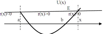
R(x) = E – U(x), 9 = √ vu .
Fig 1. Potential Well, the dependence between potential energy of elementary particles to the distance x
In the turning points: g +o- = a +o- > 0, g +s- %
a +s- w 0 . In regions x < a and x>b the wave function must decay to infinity. In regions between the turning points a < x < b the wave function has oscillatory character. That corresponds to the following notations:
In region of x < a. 5 % yh, 5= A> v, In region of a<x<b, 5=A1w+A25 , 5= A1iqw y i; ^ ,
In region of x > b. 5 = Bu, 5 = z>!a .
Here A, A1, A2, B – are arbitrary constants; w, u, v-
inserted in the previous point as the precise particular solutions of wave equation.
The requirement of smooth transition of wave function across the turning point leads to an algebraic system of equations with respect to the arbitrary constants.
A1w(a) + A2^ +o- = Av(a),
A1iq(a)w(a) A2i; (a)^ (a) = A> (a)v(a),
A1w(b) + A2^ (b) = Bw(b),
A1iq(b)w(b) A2i; (b)^ (b) = B>!(b)u(b).
The condition of quantization is to reduce the determinant of the system to zero. We have
>!(b)> (a)Im(w(a)^ (b)) > (a)Re(w(a); (b)^ (b)) >!(b)
Re(q(a)w(a)^ (b)) Im(q(a)w(a); (b)^ (b))=0 (47) In correspondence with the results of the previous point we introduce the following values:
W(x) = J@ {U?T7
q (a) = pqJ@
Q
r , q(b) = ptJ @Qr, >!(b) = pt , > (a) =pq.
Then by further simplification we can reduce the condition (47) to the following:
Re|JINi < ;MIqt fn=}=0. (48)
Emphasizing once again that here by q we mean the precise solution of Riccati’s complex equation (16) with boundary conditions in the turning points: arg q(a) = ~ 6⁄ , arg q(b) = ~ 6⁄ that’s why the integral of q should be transformed to:
;MI t
q = |!<; A6+7-8 !
?= A
@ ?•
?} MI
t
q = ! <; A 6+7-8
!
?=
t
q dx +@‚jƒƒ{„ +
f
n .
Now, the equality (48) could be written in the following form:
Re|JIN@ qt<; A 6+7-8 !?= MI} =0.
Hence, we obtain the final form of the precise quantization condition
!…J <; A 6+7-8
!
?=
t
q MI=~ <j A!=,n=1,2, (49)
The advantage of the composed record is namely, just from this shape results different approximation forms of quantization condition. In fact if Q is some asymptotic solution of Riccati’s equation, i.e. if q = Q + 0(9 ),
It is easy to be convinced, that
!
<; A 6+7-8 !?= = !<† A 6+7-8 ‡!= + O(9\ !) !
So if we put q ~F6+7-8 in (49) we immediately obtain the well-known Bohr-Sommarfeld’s semiclassic condition for quantization.
It should be noted that the traditional WKB- method also gives precise quantization condition [see [4]] which is called Wentzel’s quantization condition. But this condition includes within itself the whole asymptotic series, consequently the coefficient r(x) is assumed to be able to be analyzed. The merit of condition (49) is that, it doesn’t require from r(x) more than the solvability of Riccati’s Equation. It should be noted also, that the condition (49) is
brought here for the first time (as far as the authors of this paper know).
Let us now see how the eigenfunctions appear. Considering quantum condition (49) and boundary values, it is easy to obtain the following correlations between the arbitrary constants:
A1 =AJ Q
‰, A2 = y! =AJ@Q‰ ,
B = + 1-\AŠƒ{
ƒ„JIN | ‹Œ <; A
6+7-8
!
?= MI
t
q }.
Respectively, after simple transformations we obtain the expression of the wave function.
5= A1w+A2^ = 2AFpq…J√?! JINi |! q7<; A6+7-8 !?= MI f
4}, or
5 = 2AFpq‹Œ√?! JIN i |! q7<; A 6+7-8 ?!= MI Af4} .
4. Overcoming the Quantum
Mechanical Particles of Potential
Barrier
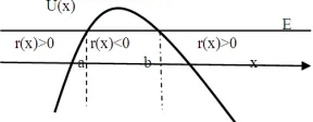
The geometric interpretation of the problem is illustrated in figure 2. In the turning points:
It is assumed that, at the left side of the potential barrier, the wave function is represented as the superposition of the ingoing and reflecting waves, whereas at the right side of the barrier only one wave passes. Now it is required to derive the formulas for calculating the coefficients of reflection and passage.
Fig 2. The potential barrier , dependence between potential energy to distance x.
Thus, for the three space regions, divided by two turning points, the wave function and its derivative can be written as follows
In the region of x<a,5= A1w+A2^ 5′=A
1iqw A2i; ^ ,
In the region of a < x < b, 5 = B1u + B2v, 5′ = B
1>!u +B2> v,
In the region of x > b, 5 = C ^Ž, 5′= C i ;Ž^Ž .
Here, as mentioned before, A1, A2, B1, B2, C – arbitrary
constants; w, u, v, ^Ž particular solution of wave
equation.
In the turning point, the wave function, and its derivative must be continuous. Therefore
In the point x = a
A1w(a)+A2^ (a)=B1u(a) + B2v(a)
A1iq(a)w(a)–A2i; (a)^ (a)= B1>!(a)u(a)+B2> (a)v(a) (50)
In the point x = b
B1u(b)+B2v(b)=C^Ž(b) (51)
B1>! + B2> (b)v(b) = C i;Ž(b)^Ž (b).
We introduce the following matrices
K = • ^+o-i;+o-^+o- ^ +o-+o-^ +o-•,
L = • >a+o-
h+o-!+o-a+o- > +o-h+o-• ,
R = • >a+s- h+s-!+s-a+s- > +s-h+s-•.
Now, the systems (50),(51) could be written as follows
K ‘y!
y ’ = L ‘zz ’! ,
R ‘zz ’! = ‘ i;1
Ž +s-’ C ^Ž+s-.
By excluding from these equalities, the constants B1, B2, we
obtain the following matrix relation
‘y!
y ’ = M ‘ i;1Ž+s-’ C ^Ž+s-,
Where, M = “ !L … !.
We calculate the elements of matrix M, and inserting the previously adopted values of
w (x) =J@{U?T7, u(x) = J {UB T7, v(x) = J{UB MI,
q(a) = pq J @
Q
r , ;Ž+s- =ptJ@Qr,
>!+o-=> +o-=pq,>!(b)=> +s-=pt, (53) ^Ž+I- = J@ ?”T7
U
„ .
As a result, after further algebraic operations, the piecewise notation of matrix equality (52) will be in the form of
A1 = !@<√3J B T7 „
{ !
√l J B[U
„
{ =C ,
A2 = !@ <√3 J B [U „
{ A !
√lJ B[U
„
{ =J@Q‰ C .
Here, as we know,>!,> denote the single pair of precise
solution of Riccati equation (17),(18) with boundary conditions (53) . In order to have the right for substituting them with some approximate solutions, it is necessary to represent their integrals in the form of
>!MI t
q = @‹jƒƒ{„ +
! <>
! 6+7-8 B!= MI
t
q ,
> MI t
q = ! ‹jƒƒ{„ +
! <> 6+7-8
!
B= MI
t
q .
Temporarily, interpreting
–! = ! qt<>! 6+7-8 B!= MI,
– = ! qt<> – 6+7-8 B!=MI,
And demonstrating that, indeed in our case the equality is established as
–! = – = – !
It is now a simple matter to conclude identities from Riccati’s equations (17), (18).
>! > = —‹j+>!A > -˜′ ,
6+7-8 <
! B
!
B= =<‹j ™ !
B A
!
Bš=
′
,
Therefore
–! – = ! qt|+>! > - 6+7-8 <B! B!=}MI =
Here, of course the boundary conditions (53) have been considered.
Now the amplitude correlations (54),(55) can be presented as follows
A1= !@Šƒƒ„
{™√3J
œ !
√lJ œš k, (56)
A2=!@Šƒƒ„
{™√3J
œA !
√lJ œš J@f l⁄ k. (57)
It is interesting to write down in explicit form the main members of asymptotic expansion of wave function from the left side and the right side of potential barrier. We have for 9 E 0 from the left side of the barrier (x < a )
5=A1w+A2^ ~√Ÿ•ž J@ ŸT7 U
{ +•
√ŸJ@ ŸT7
U
{ , (58)
From the right side of the barrier ( x > b )
5=C^@~√ŸO¡ J @ ŸT7
U
„ , (59)
Where, k(x) = F6+7-8 = √ vu F¢ •+I- .
y¡!=F;+o-A1,y¡ =F; +o-A2,k¡=F;Ž +s-C. (60)
The first term in asymptote (58) represents the wave reflected from the barrier, while the second term represents the ingoing wave on the barrier. The asymptote (59) is the essence of the wave penetrated through the barrier.
The ratio be the amplitude of the reflection and passing through waves to the amplitude of the ingoing wave i.e.
Г=• • ,T=• O¡, (61)
are called the coefficients of reflection and the coefficient of penetration respectively.
The correlations (56), (57), (60) give those coefficients the following precise formulas
Г=i √l £¤ √‰£"¤
√l£¤
√‰ £"¤
, (62)
T=√l £¤
√‰£"¤
. (63)
We see that, the coefficients Г and T are related to each other by an equality
|Г| +|¥| =1 (64) This includes within itself an important physical property of wave flux density conservation: The density of the ingoi ng flux on the potential barrier equals to the sum of the den sities of the reflecting flux from the barrier and that of passi ng through it. If for –, we use its main asymptotic approximation
–~ qt¦+I-MI % √ vu F•+I- ¢qt MI,
So for Г and T we obtain the following asymptotic formulas:
Г~i! ‰£" U[U „ {
! ‰£" {„U[U, (65)
T ~√l £"{„U[U
! ‰£" {„U[U. (66)
In case when the turning points are sufficiently far away from each other, i.e. when the height of the potential barrier considerably exceeds its own kinetic energy of attacking on the barrier particle we can use the following approximations:
Г ~ i <1 lJ {„7T7=,
T ~√lJ {„7T7 , |Г| ~ 1 |¥| .
5 Conclusions
In the present work the following new results have been obtained:
1. Special conditions (46a), (46b) covering the solution of Riccati’s equation in turning points have been deduced.
2. Precise condition of quantization (49) for obtaining the own energy values of Schrödinger‘s operator has been derived.
3. The precise (62), (63) and the approximated (65), (66) formulas for the reflected and the passage coefficients of potential barrier’s quanta-mechanical particles have been deduced.
References
[1] J. Heading.” An introduction to phase-integral method” Mir publishers,1965
[2] N Fröman and P.O Fröman JWKB “Approximation contribution to the theory” Amsterdam, North-Holland publishing company, 1965
[3] N.Fröman and P.O. Fröman “On Ventsel’s proof of the quantization condition for a single-wall potential”. J. of Mathematical Physics. University of Uppsala, Sweden vol.18.No1, 1977, pp.96-99.
[4] N.E.Tsapenko “New formulas for approximate solution of the one-dimensional wave” .Differential Equations, 1989, Minsk, vol.25.No.11, pp.1941-1946.
[5] N.E.Tsapenko “Plane electromagnetic waves in heterogeneous medium approximation regarding relative rate of change of wave resistance”. Laser and Particle Beams, 1993, vol.11No 4, pp.679-684.