Mathematical Approach for Pressure Loss Determination in Oil and Gas Pipelines

(1)

Mathematical Approach for Pressure Loss Determination in

Oil and Gas Pipelines

Ajoko, Tolumoye John*

1

_{, Kilakime Tari Amawarisenua}

2

_{Apresai, Ernest Peretiye}

3 Department of Mechanical/Marine Engineering, Faculty of Engineering, Niger Delta University, Wilberforce Island, Bayelsa State, Nigeria

ABSTRACT

The drawback caused by pressure loss in fluid flowing along oil and gas pipelines in the crude oil industry cannot be over emphasized. Thus, the functionality of industrial devices like chemical reactors, power generation units, refrigeration system, oil wells, and pipelines depends on pressure losses; however valve points and orifice are set to serve as monitoring tools to curb these challenges temporally. Therefore, the design of a well-studied fluid carrying vessel without the integration of valve system and orifice to yield maximum efficiency is a target. Hence, the mathematical approach to determine pressure loss in pipes carrying fluid from one point to the other is studied and solutions are proffered on how pressure loss could be determined with the aid of mathematical analysis. A simple convergent – divergent venturi-meter laboratory test rig was used, where manometric tube reading was collected for analytical purpose by means of some governing equation. Established results show the effectiveness of the employed methodology. Also results attest that pressure loss is consequently of poor quality installation, inadequate pipe alignment causing internal surface roughness leading to high friction of the flowing fluid.Keywords: Research Paper, Technical Writing, Science, Engineering and Technology.

Keywords: Flow rate, Pressure loss, Throat, Velocity head, Venturi-meter

I. INTRODUCTION

Pressure loss in multiphase flow across pipes connection in engineering design has created attention for research and it is a challenge yet to be solved; though the idea of these losses in valve points and orifice along the pipe determines and control the functionality of industrial devices, such as chemical reactors, power generation units, refrigeration component like the capillary tube in the expansion unit, oil wells, and pipelines. In a general view, pressure loss in pipes is the pressure difference between two points of a flowing fluid inside the pipe arrangement. It can easily occur as a result of frictional forces caused by resistance to flow which acts on a flowing fluid. However, the major determinants to measure the resistance to fluid flow are velocity and viscosity of the fluid. Thus, the concept behind the evaluation of pressure loss in fluid flow includes friction factor, coefficient of discharge, loss coefficient and valve coefficient, etc.

Different approaches for the determination of pressure loss has been extensively studied; investigation shows

that pressure loss prediction by means of correlations and published correlations based on packing geometry allows for the prediction with stratified and annular type flows with an accuracy of 20% [1]. In a contrary view, inadequate and insufficient theoretical data based on slurry flow in circular tube will lead to wrong prediction of frictional pressure losses due to limited number of correlations. However, accurate prediction of pressure losses is essential for successful treatment which avoids premature screen out of materials. Infact, to test the predictive capacity some vital properties of the pipe are considered for accuracy, they are such as the ambient pipe pressure, specific expansion ratio, pipe diameter, volume equalized power law indices [2]−[4].

(2)

devices such as orifice, valves and other machineries in the wellbore and pipelines. The basic concepts and ideas used to correlate the pressure drop in the various fluid flow situations is the frictional pressure drop expression in pipelines; where frictional pressure drop is a dependent of friction factor, length and diameter of pipeline; and the density and velocity of the fluid [6]. Another mathematical expression is the coefficient of discharge which is the ratio of actual discharge to that of ideal discharge based on frictionless flow as expressed in Bernoulli equation. Others are pressure loss coefficient and valve coefficient; nevertheless, in all cases the pressure drop is mathematically related to the correlating parameters [1], [7], [8].

Currently, the world economy lies on oil and gas resources exploration, hence creating the deep-water drilling technology where circulating pressure loss which is of wellbore pressure loss and additional pressure loss is a critical factor retarding the operation; though it is acknowledged that wellbore pressure loss represents a significant quantity in circulating pressure loss and it is analytically dependent on the determination of frictional coefficients and flow regime [9]. Thus, pressure loss or drop can also be as a result of leakage along pipelines conveying gas or oil from one point to another. This has resulted to the introduction of two types of approaches to identify leakage in a gas pipeline; they are physical inspection and mathematical model with numerical simulation.

The means of physical inspection method can result in an accurate detection of the location and the size of the leak because it has to do with gas sampling, oil and flow rate monitoring, acoustic/optical, and satellite-based hyper-spectral imaging but it is at the expense of shutting down the production process which may result to high cost and long-time duration to access the degraded portions mostly in long distance pipeline. However, the mathematical model simulation approach is a quicker evaluation method with the aid of some related governing equations though with higher uncertainties [10].

Similarly, the study of pressure loss in double – phase flow through thin and thick orifices have been analysed with multi-flows (air-water flow) in horizontal pipes with the aid of Computational Fluid Dynamics (CFD) calculations, using the Eulerian–Eulerian model; and

was proven reliable with simulation results [11]−[14]. In the laboratory, the venturi – meter is one of the most commonly used devices for the measurement of flow rate to determine the pressure drop in pipes. Hence, extensive work has been performed by scientists on optimum meter design and the performance of the meter has been studied in critical flow. Also, the effects of piping configurations and discharge coefficients have been analytically and experimentally determined for various venturi geometries [15]−[17]. The discharge coefficient of water and of gas is obtained separately in the venturi – meter with uncertainty of 0.74% and 1.23% respectively with the use of the relevant equations which is proven to be better in consideration of earlier studies according to a review literature [18], [19].

Therefore, the present study on mathematical approach to determine pressure loss in oil and gas pipelines is based on flow measurement such as pressure losses and coefficient of discharge in a laboratory venturi – meter. All results obtained in the study are considered feasible because the test rig used fulfils all necessary condition of the real pipeline setting.

II. DESCRIPTION OF THE VENTURI – METER

Figure 1 is an assembly of venturi – meter manufactured out of aluminium product, manometer tube and manifold supported on a base mounted on adjustable screwed feet. The intake of water is through the bench supply valve and it passes through a flexible hose into the meter. At the downstream of the control valve is a flexible hose leading to the measuring tank. Meanwhile, at various points along the length of the convergent – divergent passage of the venturi meter is connected to piezometer tubes drilled into the wall and further connected to vertical manometer tubes mounted in front of a scale marked in millimetres. The manometer tubes joined at their top ends has a common manifold at its left end is responsible to control the air flow by a small air valve at the opposite end.

The measurement of flow rate is by weighing technique as detailed in the hydraulic bench manual and pressure tapping in the venturi – meter; readings are obtain at the entrance, throat and exit of the convergent – divergent pipe tube [20], [21]. While this is in progress, values of

hA and hD are read from scale. Similar readings may be

(3)

Roughly equally spread maximum range of 320mm to zero being adequate for the purpose. The corresponding flow rate should be measured for each value of (hA – hD)

[20]. The large amount of tapping on this experimental tube determines discharge quantities and shows the distribution of pressure along the length of the tube passage.

Figure 1. Layout of Venturi – Meter

III. EXPERIMENTAL PROCEDURE

The rate of flow is measured by a weighing technique in the setup rig as the valve at the end of the piezometer manifold is open to the atmosphere. This test is carried out for both small and large flow rates where 1 – 4 litres and 5 – 10 litres were used respectively for the corresponding practical test. The motor pump is started and the valve at the end of the venturi – meter is gradually close to bring the level of the water in the manometers to about half way along the tube making it to an equal level. Then a small flow runs through the venturi – meter is identified; thus corresponding readings for points A, D and L are observed and records are taken against a stop watch time as shown in figure 2.

Certainly, as the two valves are opened gradually points A and D are set to new level hence flow measurement process is repeated to record values of A, D and L. This process is continuously carried out until the maximum possible difference of points A and D is obtained with their corresponding readings at entrance (A), throat (D) and exit (L) is recorded for mathematical analysis.

Figure 2 : Dimensions of venturi – meter and positions

of Piezometer tubes

IV. MATHEMATICAL ANALYSIS

In order to analyse correctly the pressure losses along a convergent – divergent pipe flowing with fluid, some governing equations are considered to determine the following performance parameters. Therefore, using the notation on figure 3 where h is the piezometric reading

in the manometer; V and A are velocity and cross

sectional area at a point in the venturi – meter according to the Bernoulli’s theorem in equation 1 and continuity equation in equation 2. The cross – sectional diameter of the venturi-meter for sections A, D and L are 26, 16 and 26mm respectively.

Figure 3: Notation on venturi – meter and Piezometer

tubes (A, D & L)

+hA = +hD = +h (1)

aA VA= aD VD = aL VL = Q (2)

(4)

–

⁄ = { }

2

− { }2 (3)

From these,

× ( )

2

+hA =

+hD (4)

VD=√

– ⁄ (5)

Q = a_√ –

⁄ (6)

Q = √ _–

⁄ (7)

∆P=

ρV

2

(8)

q = √ ∆ (9)

K = ∆

⁄

(10)

q = √∆ (11)

Where ∆P is pressure drop in orifice plate, q is volumetric flow rate, L and D is length and diameter of the pipeline respectively.

V. RESULT PRESENTATIONS

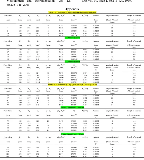
A recall of the fundamental equations of flow measurement gives the ideal pressure distribution along the venturi – meter as a fraction of the velocity head at the throat. Hence, tabulated results for small and large flow rates are presented on tables 1 and 2 respectively in the appendix. Using the mathematical expressions above for the three strategic points which are the entrance, throat and exit manometric tubes represented with point A, D and L along the venturi – meter tube are used for the star plot in the figures 4 and 5.

The pressure losses in the venturi are found from actual experimental values, where losses in a straight pipe are subtracted from the losses caused by the venturi.

Meanwhile, to determine the actual pressure losses of the flow meters in the system; the flow difference between the inlet flow to the contraction section otherwise known as the throat of the pipe and the flow from the throat to the outlet section is considered and analysed mathematically. However, the analysis are presented on a graphical plots as shown in figures 4 and 5 for both small and large flow conditions. These star plots shows pressure loss coefficient versus distance from inlet to contraction section and throat to exit along the tube.

Figure 4: Pressure loss Coefficient versus Length of

Venturi-meter for large flow

Figure 5: Pressure loss coefficient versus length of

venturi-meter for small flow

Graphical illustration of pressure loss coefficient against velocity head fraction at the throat and time of flow rate separately is presented in figures 6 and 7 respectively. Thus, figure 8 is a demonstration of different flow rate Q, against the difference in distance, (hA – hD)1/2 between

inlet and the throat along the venturi – meter. -0.6

-0.5 -0.4 -0.3 -0.2 -0.1 0.0

0 20 40 60 80 100 120 140 160

Length of venturi-meter (mm)

P

re

ss

u

re

lo

ss

c

o

ef

fi

ci

en

t (

k

)

5 - litres f low via Inlet to throat 5 - litres f low via throat to exit 7 - litres f low via Inlet to throat 7 - litres f low via throat to exit 9 - litres f low via Inlet to throat 9 - litres f low via throat to exit

-0.8 -0.7 -0.6 -0.5 -0.4 -0.3 -0.2 -0.1 0.0

0 20 40 60 80 100 120 140 160

Length of Venturi-meter (mm)

P

re

ss

u

re

L

o

ss

C

o

ef

fi

ci

en

t

(K

)

(5)

Figure 6: Pressure loss coefficient versus velocity head fraction at the throat

Figure 7: Pressure loss coefficient versus time of flow

rate

Figure 8 : Flow rate Q versus difference in distance, (hA

– hD)1/2

VI. DISCUSSION OF RESULT

In consideration of the piezometer tubes along the venturi-meter of different dimensions as shown in figure 2; two complete sets of readings are analysed for the two typical flow rates of fluid along the pipe system. It is noticed by the direction of flow that the fluid starts its flow from piezometer A at distance 0mm to B covering 20mm. As it flows along C, D and at the throat it covers distance 32mm, 46mm and 54mm respectively. A

similar analysis of distance covered by the fluid for the second flow rate is shown in the tables above.

Therefore, by expressing piezometric head changes hA –

hL as a fraction of the velocity head at the throat, results at different discharges become directly comparable in figures 4 and 5. It is seen that the analysed experimental values as used in the star plot follows the curve path quite well to the throat with a steadily increasing loss of energy becomes apparent as the fluid flows along the venturi-meter. The pressure loss coefficient, K is a total dependent of the fraction of the velocity head on the contraction section of the venturi in the graph of pressure loss coefficient against the velocity head fraction as shown in figure 6. The pressure loss increases as the fluid tends to the throat of the pipe, though it is important to note that the pressure loss for both conditions falls above the stipulated range of 5 – 20% which is likely caused by poor installation of pipes with inadequate alignment resulting to high frictional losses in the internal connection of the pipes. However, at the point of constriction of the flow or the throat in the venturi, corresponding increase of velocity is produced with drop in pressure which is a function of the flow.

Thus, the constriction is formed at the downstream; hence the difference between the upstream and downstream flow pressure is a function of the flow rate, Q which is plotted against difference in distance between the upstream and downstream, along the pipe system as shown in figure 8. The interpretation of the graphical plot means that as hA – hD gets larger, the flow rate increases because it is closer to the constriction point at the downstream. Contrary, hA – hD will be small with little amount of flow rate at the upstream of the system. Meanwhile, the graph plot in figure 7 analyses the steady increase of pressure loss in the system with respect to increasing time of flow rate with similar pattern of curve.

VII. CONCLUSION

The determination of pressure loss in oil and gas pipelines using mathematical analysis was justifiable due to the following reasons as validated in the open literature. The established results were contrary to the bench mark, meaning pressure loss values were out of the range satisfying the existence of pressure loss in the evaluated laboratory pipe system. Thus, confirming -0.8

-0.7 -0.6 -0.5 -0.4 -0.3 -0.2 -0.1 0.0

0 10 20 30 40

Velocity Head Fraction at Throat

Pre

ssu

re

L

o

ss

(K)

2 - litres flow rate determination test 3 - litres flow rate detrmination test 4 - litres flow rate determination test 5 - litres flow rate determination test 7 - litres flow rate determination test 9 - litres flow rate determination test

0 20 40 60 80 100 120

-0.25 -0.20 -0.15 -0.10 -0.05 0.00

Pressure Loss Coefficient Loss (K)

T

im

e

o

f

F

lo

w

R

a

te

(

s

e

c

)

flow rate with 2 - litres flow rate with 3 - litres flow rate with 4 - litres flow rate with 5 - litres flow rate with 7 - litres flow rate with 9 - litres

0.0E+00 1.0E+04 2.0E+04 3.0E+04 4.0E+04 5.0E+04 6.0E+04 7.0E+04 8.0E+04 9.0E+04 1.0E+05

0.0 1.0 2.0 3.0 4.0 5.0

(hA - hD)1/2

Q

(m

m

3

/5

)

(6)

improper pipe alignment with weak and rough internal finish having high friction condition which yields more than 5 – 20% of pressure loss in the pipe under study. The result of pressure loss coefficient “K” as a total dependent of the fraction of the velocity head on the contraction section of the venturi as illustrated in figure 6 confirms and supports the open literature which attests that pressure loss is as a result of frictional forces caused by resistance to flow which acts on a flowing fluid measured by the fluid velocity and viscosity. Established results confirms the mathematical approach applied as a capable tool to determine the pressure loss at joint or valve units of two or more pipes bend corners and intersection points of bigger and smaller pipe connection along oil and gas pipelines.

Consequently, the relevance of the application is

fulfilled by the use of venturi-meter experimental test rig as shown above with one end of the piezometric tubes drilled into the venturi wall and the other end connected to manometer tubes A – L scale marked in millimetres. Therefore, the possibility of achieving the objectives of the research is attainable and the application can be extended to any other oil and gas pipeline provided the governing equations are utilized and analysed at the relevant sections along the pipeline.

VIII. REFERENCES

[1]. P. L. Spedding, E. Benard, and G. F. Donnelly,

"Prediction of pressure drop in multiphase

horizontal pipe flow", International

Communications in Heat and Mass Transfer, vol. 33, pp. 1053-1062, 2006.

[2]. D. Markus, "Packing Pressure Drop Prediction at Low Operating Pressure: Is There Anything New", Distillation Topical Conference, AIChE Spring Meeting, Sulzer Chemtech Ltd, San Antonio, Texas, 2013.

[3]. S. S. Ali, and H. K. Ahmed, "A Statistical

Evaluation of the Frictional Pressure Losses Correlations for Slurry Flow", Journal of Geological Resource and Engineering, vol. 2, pp. 69-76, 2014.

[4]. B. S. Gardiner, B. Z. Dlugogorski, and G. J.

Jameson, "Prediction of Pressure Losses in Pipe Flow of Aqueous Foams," Ind. Eng. Chem. Res, vol. 38, pp.1099-1106, 1999.

[5]. V. G. Ainshtein,"A new Approach to

Determination of pressure Losses", Chemistry and Technology for Fuels and Oils, vol. 37, issue 1, pp. 21 – 22, 2001.

[6]. K. R. Manmatha, J. Jibanananda, and K. D.

Sukanta,"Mathematical Modelling of Two-phase Flow through Thin Orifices in Horizontal Pipes," Proceedings of ICTACEM, Kharagpur, India, 2010.

[7]. J. S. Gudmundsson, "Pressure Drop in Petroleum Production Operations," Norwegian institute of

Technology", Department of Petroleum

Engineering and Applied Geophysics, Tech. Rep.1-3, 1995.

[8]. K. B. Lalit, "Flow and Pressure drop of Highly Viscous Fluids in small Aperture orifices," MSc. thesis, Georgia Institute of Technology, June 2004.

[9]. Z. Yujia, and W. Zhiming, "A Comprehensive

Model for Circulating Pressure Loss of Deep-water Drilling and Its Application in Liwan Gas Field of China", Res. J. App. Sci. Eng. Technology, vol. 7, issue 8, pp.1678-1688, 2014.

[10]. L. Kegang, H. Guoqing, N. Xiao, X. Chunming,

H. Jun, P. Peng, and G. Jun, "A New Method for Leak Detection in Gas Pipelines", Oil and Gas Facilities, pp.97-106, 2015.

[11]. K. R. Manmatha, and K. D. Sukanta, "Single-Phase and Two-"Single-Phase Flow through Thin and Thick Orifices in Horizontal Pipes", ASME J. Fluids Eng, vol. 13, issue 9, 2012.

[12]. K. R. Manmatha, K. D. Sukanta, "Numerical

Modeling of Pressure drop due to Single-phase Flow of Water and Two-phase Flow of Air-water Mixtures through Thick Orifices", International

Journal of Engineering Trends and

Technology,vol. 3, issue 4, pp.554-551, 2012. [13]. S. Z. Jose, "Multiphase Analysis of three-Phase

(gas-condensate-water) Flow in Pipes" PhD thesis, Pennsylvania State University, 2006.

[14]. E. B. Christopher, Fundamentals of Multiphase

Flows, California Institute of Technology

Pasadena, California Cambridge University Press, 2005.

[15]. J. Thomas, C. J. Robert, and N. K. Lloyd, 1968, "Performance of a Venturi Meter with Separable Diffuser", National Aeronautics and Space Administration, 1968.

[16]. General Instruments Consortium (2008) "Flowing

(7)

[17]. H. Abdel-Alim, "Part 2: Steady – State Flow of Gas through Pipes," homepage on PE 607: Oil and Gas Pipeline Design, Maintenance and Repair. Online]. Available: http:// www.eng.cu.edu.eg (Accessed on the 23th December, 2015).

[18]. M. J. Reader-Harris, W. C. Brunton, J. J. Gibson,

D. Hodges, and I. G. Nicholson, "Discharge coefficients of Venturi tubes with Standard and

Non-standard Convergent Angles", Flow

Measurement and Instrumentation, vol. 12, pp.135–145, 2001.

[19]. P. M. Gary, "Flow Measurement in Pipes"

Unpublished BIE 5300/6300 Lectures, pp.141 – 152..

[20]. Engineering Faculty, "hydraulic bench manual",

(Unpublished Fluid Mechanics

Laboratory/Workshop Manuals) Niger Delta University, Bayelsa State, Nigeria, 2013.

[21]. T. J. Dudzinski, R. C. Johnson, and L. N. Krause,

"Venturi Meter with Separable Diffuser", J. Basic Eng, vol. 91, issue 1, pp.116-120, 1969.

Appendix

Table 1:- Collection of Small flow rates(2 - litres of water)

Flow Time hA hD hL hA -hD (hA -hD)1/2 Q VD2/2g Pressure length of venturi length of venturi

(sec) (mm) (mm) (mm) (mm) (mm) (mm3/5₎ _Loss _{(Inlet - Throat)} _{(Throat - outlet)}

(k) (mm) (mm)

2 320 310 322 10 3.162 17982.4 16.10 -0.1243 0 156

4 300 292 303 8 2.828 16084.0 12.88 -0.2330 20 136

8 280 274 283 6 2.449 13929.1 9.66 -0.3107 32 106

14 260 256 263 4 2.000 11373.1 6.44 -0.4660 46 88

22 240 238 241.8 2 1.414 8042.0 3.22 -0.5592 54 76

3 - Litres of water

(k) (mm) (mm)

26 320 307 323 13 3.606 30754.7 20.92 -0.1434 0 156 27 300 291 304 9 3.000 25589.4 14.49 -0.2761 20 136

30 280 275 283 5 2.236 19073.2 8.05 -0.3728 32 106

35 260 257 262.4 3 1.732 14774.1 4.83 -0.4970 46 88

42 240 239 241 1 1.000 8529.8 1.61 -0.6213 54 76

4 - Litres of water

(k) (mm) (mm)

46 320 305 324 15 3.873 44047.8 24.14 -0.1657 0 156 48 300 288 306 12 3.464 39397.5 19.31 -0.3107 20 136 52 280 271 286 9 3.000 34119.2 14.49 -0.4142 32 106 58 260 256 263.5 4 2.000 22746.2 6.44 -0.5436 46 88 66 240 239 241.1 1 1.000 11373.1 1.61 -0.6834 54 76

Table 2:- Collection of Large flow rates (5 - litres of water)

(k) (mm) (mm)

55 320 300 322 20 4.472 63577.5 32.19 -0.0621 0 156 57 310 297 312 13 3.606 51257.8 20.92 -0.0956 20 136 61 300 291 302 9 3.000 42649.1 14.49 -0.1381 32 106

67 290 285 292 5 2.236 31788.7 8.05 -0.2485 46 88

75 240 237 242 3 1.732 24623.4 4.83 -0.4142 54 76

Water Quantity of 7 - Litres

(k) (mm) (mm)

79 320 300 323 20 4.472 89008.4 32.19 -0.0932 0 156 80 310 295 313 15 3.873 77083.6 24.14 -0.1243 20 136 83 301 290 304 11 3.317 66010.4 17.70 -0.1694 32 106

88 290 286 292 4 2.000 39805.8 6.44 -0.3107 46 88

95 290 289 291 1.4 1.183 23549.4 2.25 -0.4438 54 76 Water Quantity of 9 - Litres

(k) (mm) (mm)