doi:10.5194/nhess-12-1393-2012
© Author(s) 2012. CC Attribution 3.0 License.
and Earth
System Sciences
Verification of precipitation forecasts of MM5 model over Epirus,
NW Greece, for various convective parameterization schemes
O. A. Sindosi1, A. Bartzokas1, V. Kotroni2, and K. Lagouvardos2
1Laboratory of Meteorology, Department of Physics, University of Ioannina, Ioannina, Greece
2Institute of Environmental Research and Sustainable Department, National Observatory of Athens, Athens, Greece Correspondence to: A. Bartzokas (abartzok@uoi.gr)
Received: 15 April 2011 – Revised: 22 December 2011 – Accepted: 2 March 2012 – Published: 9 May 2012
Abstract. The mesoscale meteorological model MM5 is ap-plied to 22 selected days with intense precipitation in the region of Epirus, NW Greece. At first, it was investigated whether and to what extend an increased horizontal resolu-tion (from 8 to 2 km) improves the quantitative precipitaresolu-tion forecasts. The model skill was examined for the 12-h accu-mulated precipitation recorded at 14 meteorological stations located in Epirus and by using categorical and descriptive statistics. Then, the precipitation forecast skill for the 2 km grid was studied: (a) without and (b) with the activation of a convective parameterization scheme. From the above study, the necessity of the use of a scheme at the 2 km grid is as-sessed. Furthermore, three different convective parameteri-zation schemes are compared: (a) Betts-Miller, (b) Grell and (c) Kain-Fritsch-2 in order to reveal the scheme, resulting in the best precipitation forecast skill in Epirus. Kain-Fritsch-2 and Grell give better results with the latter being the best for the high precipitation events.
1 Introduction
Precipitation is one of the most difficult parameters to fore-cast in numerical weather prediction (Olson et al., 1995; Wang and Seaman, 1997). The question if an increase in horizontal resolution can produce more skilful precipi-tation forecasts is discussed, among others, by Ducrocq et al. (2002), Lagouvardos et al. (2003), Kotroni and Lagou-vardos (2004). These authors pointed out that the subjective impression of the forecaster is that the fine grid precipitation fields are much closer to the real precipitation fields. Never-theless, it seems that even when using very fine resolution, the models are still unable in many cases to reproduce the observed high precipitation amounts. Other researchers have
found that, in anomalous terrain, in order to generate a re-alistic orographic representation of precipitation structures, a high resolution grid is necessary (Colle and Mass, 2000). Also, mesoscale modelling studies have shown that when models use a relatively high resolution (down to ∼10 km) they can capture more of the observed mesoscale features (Zhang et al., 1989; Bruintjes et al., 1994; Colle and Mass, 1996; Gaudet and Cotton, 1998).
One of the difficulties in precipitation prediction, in a mesoscale model, is the satisfactory representation of both resolved and subgrid-scale precipitation processes. The lat-ter is known as a convective paramelat-terization problem, and its challenge and complexity have been acknowledged for many years (Emanuel and Reymond, 1993; Wang and Sea-man, 1997). A wide variety of convective parameterization schemes (CPSs) have been developed and incorporated into mesoscale models (e.g. Kuo, 1974; Arakawa and Schubert, 1974; Anthes, 1977; Frich and Chappell, 1980; Betts and Miller, 1993; Kain and Fritsch, 1993; Grell, 1993; Kain, 2004). The various CPSs have been tested and compared in many experiments (Kuo et al., 1996; Wang and Seaman, 1997; Ferretti et al., 2000; Kotroni and Lagouvardos, 2001; Cohen, 2002; Mazarakis et al., 2009; Sindosi et al., 2010). As far as it concerns the high-resolution models, many re-searchers have emphasized that, in general, models are able to explicitly resolve convective systems without CPSs (e.g. Weisman et al., 1991; Carbone et al., 2002; Davis et al., 2003; Wilson and Roberts, 2006).
Fig. 1. The three nested domains used
Fig. 1. The three nested domains used.
move eastwards over the relatively warm Mediterranean wa-ters (see e.g. Alpert et al., 1990; Trigo et al., 2002; Nissen et al., 2010), favour the development of severe precipitation events over the windward NW Greece. This is why Epirus is frequently called “the gate of the cyclones to Greece”. Ioannina, a city with a population of 120 000, is the capi-tal of Epirus, located in a plateau of about 500 m altitude, in the center of Epirus. It receives, on average, 1082 mm in 124 precipitation days per year.
In order to improve as much as possible the local weather forecast and to inform the authorities and the public in case of an extreme weather event, the Laboratory of Meteorology of Ioannina University, in the frame of RISKMED project (Bartzokas et al., 2010), has implemented, since 2007, the meteorological model MM5 (Dudhia, 1993; Grell, 1994) at high-resolution. The aim of the present study is to investigate whether precipitation forecast in Epirus, an area with discrete topographic characteristics, is improved when: (i) model res-olution is increased from 8×8 km grid to 2×2 km grid, (ii) a CPS is applied in the high resolution grid (2×2 km), and (iii) different CPSs are applied. In addition, a possible de-pendence of the results on the continentality is investigated by comparing the results over three distinct areas: coastal, inland and mountainous.
The rest of the paper is structured as follows. The follow-ing session is devoted to the presentation of the methodology and the data sets used. The results of the study are analysed in Sect. 3 while one of the intense precipitation events is pre-sented analytically in Sect. 4. The last section is devoted to the concluding remarks of the study.
2 Data and methodology
As already mentioned, this study is based on the use of MM5 non-hydrostatic model, which is widely used by many in-stitutes and meteorological services around the world. The model allows the selection among a large number of pa-rameterization schemes for the various physical processes. In Ioannina University, the microphysical scheme described by Schultz (1995) and the CPS Kain-Fritsch-2 (Kain and
Fig. 2.Automatic meteorological stations in Epirus (altitudes in meters).
Fig. 2. Automatic meteorological stations in Epirus (altitudes in
meters).
Fritsch, 1993; Kain, 2004) have been adopted. After test-ing the implementation of many schemes, this selection was found to be, in general, the best for the Greek area (Kotroni and Lagouvardos, 2001, 2004). For the parameterization of atmospheric boundary layer, the scheme of Hong and Pan (1996), known as MRF scheme, is used. The selection of MRF scheme is based on findings of Akylas et al. (2007), who compared the MM5 operational forecasts over Athens with three different atmospheric boundary layer schemes. For the operational weather forecasts the following three do-mains are adopted: (a) grid 1, with 24 km horizontal grid in-crement (140×220 grid points), covering most of Europe and the Mediterranean, (b) grid 2, with 8 km horizontal grid increment (130×151 grid points), covering Greece and the surrounding sea areas, and (c) grid 3, with 2 km hori-zontal grid increment (113×113 grid points), covering the Epirus area and the northeastern Ionian Sea (Fig. 1). The one-way nesting strategy is used since the ratio of the three resolutions is not 1 over 3, which is obligatory for the two-way strategy. In all the domains, 23 not equally spaced ver-tical levels are used with most of them being in the plane-tary boundary layer for a better initialization of convection. Although, for a more accurate triggering of precipitation, a higher number of levels would be desirable, especially be-cause of the high horizontal resolution of the third domain, the settings adopted by the Ioannina University for the oper-ational use of MM5 are kept. The version of MM5 used in the University demands the same number of vertical levels in all domains, and an increase of this number would imply an impractically long simulation period because of the limited computing power. The model uses, as initial and boundary conditions, data from the GFS global model, provided by US Weather Service.
Fig. 3. Flow diagram representing the process followed. The first three rows represent the three domains and the CPS choices in each of them. In the fourth row, the techniques used for the estimation of precipitation forecasts at the locations of the stations are presented. Underneath, the abbreviations used for each process are given (for example: 8_KF2_Cre means that these results come from the 8km grid with Kain-Fritsch-2 CPS and the Cressman interpolation method). Finally, in the coloured boxes, the questions investigated in the present work by comparing results of certain procedures are shown.
Fig. 3. Flow diagram representing the process followed. The first
three rows represent the three domains and the CPS choices in each of them. In the fourth row, the techniques used for the estimation of precipitation forecasts at the locations of the stations are pre-sented. Underneath, the abbreviations used for each process are given (for example: 8 KF2 Cre means that these results come from the 8 km grid with Kain-Fritsch-2 CPS and the Cressman interpola-tion method). Finally, in the coloured boxes, the quesinterpola-tions investi-gated in the present work by comparing results of certain procedures are shown.
of the years 2009 and 2010, were selected. The selection criterion was based on three factors: the spatial extent of pre-cipitation, its intensity and the functioning of the rain gauges. These events have been simulated using: (a) the operational model chain described above, (b) the aforementioned chain but using the Grell CPS instead of Kain-Fritsch-2, (c) the aforementioned chain but using the Betts-Miller CPS instead of Kain-Fritsch-2. It should be noted that for the operational chain running at the Ioannina University, the CPS scheme is activated in all three model grids. For that reason an addi-tional experiment has been made that is identical to the oper-ational chain except that the CPS is not activated for grid 3.
In order to verify precipitation forecast, data from 14 auto-matic meteorological stations, located in Epirus (Fig. 2), are used. Other type of data, e.g. radar retrieved rainfall, are not available for this part of Greece while satellite data, given in 0.5×0.5◦resolution, are too coarse for Epirus, which covers approximately 1.5◦in latitude and 1◦in longitude. The val-idation as well as the whole research is applied for the rain amounts recorded during the two 12-h intervals of the rain days, considering the prediction values oft+12 andt+24. All model simulations are initialised at 00:00 UTC and pre-cipitation values are given at the centres of the grid boxes (Arakawa-Lamb B staggering). The forecast is launched without a spin-up time, on the one hand for homogeneity rea-sons, as all the precipitation events do not start at the same time, and on the other hand because of the routine procedure of the Ioannina University that is based on 00:00 UTC data.
Table 1. Mean Absolute Error (MAE) (mm) for: (a) 8 km grid using
the Cressman method (8 KF2-Cre), (b) 2 km grid using the Cress-man method (2 KF2 Cre), (c) 2 km grid using the 4 points method (2 KF2 4p). In all cases Kain-Frich-2 CPS is used. The best values are presented in bold.
classes cases 8 KF2 Cre 2 KF2 Cre 2 KF2 4p
(mm)
t+12
1–2.5 14 10.2 5.7 4.8
2.5–5 22 4.1 4.1 3.3
5–10 58 4.9 4.4 3.2
10–20 84 7.3 8.0 5.8
>20 99 14.4 16.1 12.4
t+24
1–2.5 13 3.1 3.3 2.6
2.5–5 24 4.8 4.6 3.4
5–10 46 7.4 5.3 4.1
10–20 72 6.9 7.8 5.4
>20 100 17.0 19.3 14.6
For the estimation of precipitation forecasts at the loca-tions of the staloca-tions, two techniques were employed: (i) the Cressman method and (ii) the method of the 4 grid points.
In Cressman method, precipitation,P, is interpolated to each observation site by using the inverse distance formula
P=(X
n=1,4
WnPn)/( X
n=1,4 Wn)
wherePn is the model precipitation at the four grid points
surrounding the observation site andWnis a weight given by Wn=(R2−Dn2)/(R
2+D2 n)
whereRis the model horizontal grid spacing andDn is the
horizontal distance from the model grid point to the obser-vational site (Cressman, 1959; Colle et al., 1999). If for a grid pointD > R, this point is not taken into account andW is set equal to 0.
In the method of the 4 grid points, the differences be-tween the observation and the model precipitation at the four grid points surrounding the observation site are calculated. Then, the model precipitation with the smallest difference from the observation is considered as the predicted value. In this way, the 2×2 km resolution may lead to a small shift in rain distribution up to 2
√
2 km=2.8 km. This method is introduced in order not to consider as incorrect a rainfall fore-cast with a spatial distribution slightly different from the ob-served one.
The verification of precipitation forecast, for each 12-h interval, is carried out separately for 5 precipitation classes with ranges: 1–2.5, 2.5–5, 5–10, 10–20 and>20 mm. For each of them, the mean absolute error (MAE) is calculated MAE=1
n n X
i=1
|Pf−Po|
wherePfis the forecasted rain value at the station site
Table 2. As in Table 1, but for Proportion Correct (PC) and Equitable Threat (ET) scores, for 5 precipitation thresholds. The best values are
presented in bold.
Proportion Correct (0–1) Equitable Threat (−1/3–1)
Thresh. cases 8 KF2 Cre 2 KF2 Cre 2 KF2 4p 8 KF2 Cre 2 KF2 Cre 2 KF2 4p
t+12
1 mm 277 0.93 0.90 0.94 0.12 0.07 0.14
2.5 mm 263 0.85 0.83 0.89 0.09 0.13 0.23
5 mm 241 0.78 0.76 0.84 0.19 0.18 0.31
10 mm 183 0.71 0.71 0.75 0.23 0.26 0.33
20 mm 99 0.77 0.77 0.84 0.31 0.29 0.44
t+24
1 mm 255 0.92 0.90 0.94 0.44 0.37 0.53
2.5 mm 242 0.89 0.85 0.89 0.43 0.34 0.44
5 mm 218 0.87 0.80 0.87 0.50 0.36 0.50
10 mm 172 0.74 0.70 0.76 0.32 0.26 0.34
20 mm 100 0.79 0.76 0.80 0.33 0.26 0.36
value andnthe number of stations with recorded precipita-tion in a specific class.
MAE determines the magnitude of the precipitation errors of the model but it does not give an insight of the frequency of precipitation events above certain thresholds. For this pur-pose, 2×2 (yes/no) contingency tables are constructed and several statistical parameters are computed (Schultz, 1995; Mesinger, 1996; Belair et al., 2000; Accadia et al., 2003; Lagouvardos et al., 2003; Federico et al., 2004; Mazarakis et al., 2009). A contingency table consists of four elements which determine the number of occurrences in which the ob-servation and the forecasted precipitation value did or did not exceed a given threshold. These elements are: H (hits), which represents the number of cases that both the obser-vation and the predicted value exceeded a certain threshold, F (false alarms), number of cases that the model predicted precipitation above the threshold but it did not occur, M (misses), number of cases that the model erroneously pre-dicted precipitation lower than the threshold, andC (correct negatives), number of cases that the model predicted cor-rectly rain lower than the threshold. In the framework of this study, contingency tables are computed for the thresholds: 1.0, 2.5, 5.0, 10.0 and 20.0 mm.
Then, in order to describe particular aspects of precipita-tion forecast performance, three categorical statistics of the contingency tables are computed: Bias score (BIAS), Pro-portion Correct score (PC) and Equitable Threat score (ET). Bias is defined as: BIAS=For/Obs=(H+F)/(H+M). It measures the ratio of the frequency of forecast events to the frequency of observed events. The perfect score is 1 and it indicates whether the forecast system has a tendency to under-predict (BIAS<1) or over-predict (BIAS>1) events. Proportion Correct is defined as: PC=(H+C)/N, where N is the total number of observations verified. It represents the fraction of predictions that were correct and it takes val-ues from 0 (worst score) to 1 (perfect score).
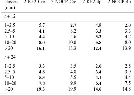
Table 3. Mean Absolute Error (MAE) (mm) for forecast with
Kain-Fritsch-2 (KF2) and without activation of the CPS (NOCP) in the 2 km grid with Cressman and 4 points method. The best values for each method are presented in bold.
classes 2 KF2 Cre 2 NOCP Cre 2 KF2 4p 2 NOCP 4p
(mm)
t+12
1–2.5 5.7 2.7 4.8 2.0
2.5–5 4.1 8.2 3.3 3.3
5–10 4.4 5.6 3.2 4.2
10–20 8.0 10.0 5.8 8.0
>20 16.1 18.3 12.4 13.9
t+24
1–2.5 3.3 3.5 2.6 2.5
2.5–5 4.6 4.8 3.4 3.9
5–10 5.3 5.5 4.1 4.4
10–20 7.8 9.9 5.4 7.5
>20 19.3 19.9 14.6 14.8
Equitable Threat score is defined as: ET=(H−E)/(H+
F+M−E)whereE=(H+M)(H+F )/N. It measures the fraction of observed and/or forecast events that were cor-rectly predicted, adjusted for hits associated with random chance. An Equitable Threat equal to 1 is a perfect score, while−1/3 is the lowest possible value.
All the categorical statistics, bias, PC and ET are com-puted for each 12-h interval and for each precipitation thresh-old.
Table 4. As for Table 3 but for Epirus only with and without activation of the Kain-Fritsch-2 CPS in the 2 km grid. For each categorical
statistic and for each method the best values are presented in bold.
Thresh. Proportion Correct (0–1) Equitable Threat (−1/3–1)
t+12 2 KF2 Cre 2 NOCP Cre 2 KF2 4p 2 NOCP 4p 2 KF2 Cre 2 NOCP Cre 2 KF2 4p 2 NOCP 4p
1 mm 0.90 0.77 0.94 0.84 0.07 0.03 0.14 0.07
2.5 mm 0.83 0.71 0.89 0.76 0.13 0.10 0.23 0.13
5 mm 0.76 0.67 0.84 0.74 0.18 0.15 0.31 0.22
10 mm 0.71 0.67 0.75 0.72 0.26 0.23 0.33 0.30
20 mm 0.77 0.76 0.84 0.82 0.29 0.28 0.44 0.40
t+24
1 mm 0.90 0.78 0.94 0.83 0.37 0.18 0.53 0.25
2.5 mm 0.85 0.71 0.89 0.77 0.34 0.15 0.44 0.24
5 mm 0.80 0.70 0.87 0.75 0.36 0.23 0.49 0.29
10 mm 0.70 0.66 0.76 0.75 0.26 0.21 0.34 0.34
20 mm 0.76 0.76 0.80 0.82 0.26 0.26 0.36 0.40
method for the high resolution (the latter is not used for the 8 km grid because of the large distances).
Then, in order to assess the role of the activation of the CPS in the high resolution grid (grid 3), on the forecasted precipitation, the simulations where the CPS is activated on all three grids are compared with the simulations where the CPS is activated in the coarse (24×24 km) and the interme-diate (8×8 km) domains only and not in the fine (2×2 km) one.
The CPS resulting to the best precipitation prediction in Epirus is revealed, by implementing, for the same rain days apart from Kain-Fritsch-2, Betts-Miller and Grell CPSs, in all domains.
Thereinafter, the 14 Epirus stations are classified, subjec-tively, in three groups based on their altitude: 4 coastal (al-titude up to 100 m), 5 inland (from 100 m to 500 m), and 5 mountainous (above 500 m) and the categorical statistics are also computed for each sub-region.
The whole procedure followed, is presented, in a concise way, in the flow diagram of Fig. 3.
3 Results
3.1 For Epirus as a whole
MAE values for the intermediate and the fine grid analyses are presented in Table 1. The results are given for each 12-h interval, for each of the 5 rainfall classes and each of the 2 interpolation methods. The number of cases for each class is also given. The best values are presented in bold. It is seen that by using Cressman method, higher resolution leads to better results (lower MAEs) only for light and moderate precipitation. However, when the 4 points method is adopted for the fine grid, the results appear considerably better for all cases.
The corresponding scores of PC and ET, for the 5 precipi-tation thresholds, are presented in Table 2. The number of cases for each threshold is also given. It is seen that for both categorical statistics, by using the Cressman method a higher resolution does not lead to better results. Ducrocq et al. (2002), who reached the same conclusions, argued that this is due to the fact that the surface observation network is generally too coarse to describe the high spatial and temporal variability of precipitation fields. Moreover, as resolution in-creases, the model is able to produce more concentrated and intense cores of precipitation. In that case, small errors in locations between the observation and forecast can produce large differences and consequently bad scores. However, in Table 2 it is also seen that by using the 4 points method, the finest grid does improve precipitation forecast for all cases. For PC, the results are better for low thresholds, i.e. when almost all rainfall events (with either light or moderate or heavy precipitation) are taken into account, while for larger thresholds (light precipitation events are excluded), the per-formance of the model is poorer. For ET, which has the equi-tability property and rates random forecasts and all constant forecasts equally, the scores are lower. The reason is that ET does not weight strongly correct forecasts of common events in order not to artificially inflate the resulting score, and in the present work, only days with extended and intense pre-cipitation over the whole Epirus are considered. ET scores would be higher if non-rainy days were also included in the analysis.
Table 5. The percentage of convective part of precipitation obtained by the use of Kain-Fritsch-2 for the two 12-h intervals (t+12,t+24).
Stations 00:00–12:00 12:00–24:00 (height in m)
Coastal
Ammoudia (1) 71 72
Arta (13) 59 66
Sagiada (48) 55 47
Igoumenitsa (75) 39 33
Inland
Koboti (105) 52 66
Paramithia (128) 57 53
Doliana (404) 38 31
Lake Isl. (472) 39 33 Ioannina Univ. (485) 37 36
Mountainous
Vourgareli (648) 18 29
Eleftherohori (650) 5 8
Trapeza (719) 30 21
Katarraktis (902) 12 20
Metsovo (1231) 20 17
Table 6. As in Table 1 but for the three different CPSs: Betts-Miller, Grell and Kain-Fritsch-2. For each grid and for each method the best
values are presented in bold.
classes 8 BM Cre 8 GR Cre 8 KF2 Cre 2 BM Cre 2 GR Cre 2 KF2 Cre 2 BM 4p 2 GR 4p 2 KF2 4p (mm)
t+12
1–2.5 8.1 8.2 10.2 9.2 11.9 5.7 7.8 9.6 4.8
2.5–5 4.9 4.9 4.1 4.5 5.3 4.1 3.9 4.4 3.3
5–10 5.1 4.7 4.9 6.4 5.1 4.4 5.1 3.3 3.2
10–20 7.8 8.2 7.3 9.5 9.1 8.0 7.0 6.6 5.8
>20 15.6 14.0 14.4 17.1 14.5 16.1 12.7 10.1 12.4
t+24
1–2.5 3.7 3.7 3.1 4.9 4.1 3.3 3.9 3.1 2.6
2.5–5 6.1 4.8 4.8 5.7 6.2 4.6 4.4 4.3 3.4
5–10 8.0 7.4 7.4 5.8 6.9 5.3 4.5 4.9 4.1
10–20 7.9 7.4 6.9 9.2 8.9 7.8 7.0 6.0 5.4
>20 15.9 15.4 17.0 19.7 17.8 19.3 14.6 13.0 14.6
apart for the lowest (1–2.5 mm). In order to explain the fore-cast improvement, without CPS, in the 1–2.5 class, simula-tion results have been examined in detail (not presented). It was found that for the light precipitation, the NOCP simu-lations have much more misses (forecast 0–1 mm) than false alarms (forecast above 2.5 mm) (comparison of NOCP with Kain-Fritsch-2), resulting in lower MAE values.
The verification of the forecasts above specific thresholds is presented in Table 4. It is seen that the PC and ET scores support the findings of MAE (estimated in classes) since the values are found better when the CPS is activated. A small exception can be seen in very high precipitation values where scores with and without CPS are more or less comparable.
For a further examination of the model performance with CPS and in order to distinguish the parameterized convection
from the explicit one, the percentage of convective precipita-tion obtained by the use of Kain-Fritsch-2 (22 days average) is presented in Table 5. It is seen that for the coastal sta-tions the percentage is very high, exceeding 50 % almost in all of them. In the inland stations this percentage is reduced to about 40 % while on the mountainous ones it is, in gen-eral, below 20 %. This last finding was more or less expected since MM5 tends to produce precipitation in the mountain regions because enough triggering is available. The moun-tains force the flow to uplift, allowing for water vapour to condensate, that is, the MM5 air column reaches saturation and, if the case, produces precipitation explicitly.
Table 7. As in Table 2 but for Proportion Correct (PC) score (0–1) and three different CPSs: Betts-Miller, Grell and Kain-Fritsch-2.
Thresh. 8 BM Cre 8 GR Cre 8 KF2 Cre 2 BM Cre 2 GR Cre 2 KF2 Cre 2 BM 4p 2 GR 4p 2 KF2 4p
t+12
1 mm 0.87 0.94 0.93 0.83 0.91 0.90 0.86 0.94 0.94
2.5 mm 0.80 0.85 0.85 0.77 0.84 0.83 0.81 0.88 0.89
5 mm 0.76 0.80 0.78 0.71 0.78 0.76 0.77 0.83 0.84
10 mm 0.69 0.72 0.70 0.67 0.70 0.71 0.72 0.76 0.75
20 mm 0.81 0.75 0.77 0.77 0.76 0.77 0.81 0.81 0.84
t+24
1 mm 0.90 0.90 0.92 0.83 0.88 0.90 0.88 0.92 0.94
2.5 mm 0.86 0.85 0.89 0.77 0.83 0.85 0.81 0.86 0.89
5 mm 0.81 0.82 0.87 0.73 0.78 0.80 0.78 0.85 0.87
10 mm 0.72 0.71 0.74 0.68 0.71 0.70 0.74 0.82 0.76
20 mm 0.78 0.80 0.79 0.79 0.77 0.76 0.81 0.83 0.80
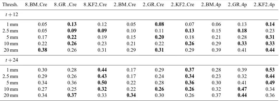
Table 8. As in Table 2 but for Equitable Threat (ET) score (−1/3–1) and three different CPSs: Betts-Miller, Grell and Kain-Fritsch-2.
Thresh. 8 BM Cre 8 GR Cre 8 KF2 Cre 2 BM Cre 2 GR Cre 2 KF2 Cre 2 BM 4p 2 GR 4p 2 KF2 4p
t+12
1 mm 0.05 0.13 0.12 0.05 0.08 0.07 0.06 0.13 0.14
2.5 mm 0.05 0.09 0.09 0.10 0.11 0.13 0.15 0.18 0.23
5 mm 0.17 0.22 0.19 0.15 0.20 0.18 0.21 0.28 0.31
10 mm 0.22 0.26 0.23 0.21 0.22 0.26 0.29 0.33 0.33
20 mm 0.38 0.26 0.31 0.29 0.31 0.29 0.39 0.41 0.44
t+24
1 mm 0.30 0.28 0.44 0.17 0.29 0.37 0.28 0.39 0.53
2.5 mm 0.29 0.26 0.43 0.17 0.24 0.34 0.23 0.32 0.44
5 mm 0.34 0.36 0.50 0.22 0.28 0.36 0.30 0.41 0.49
10 mm 0.27 0.25 0.32 0.22 0.26 0.26 0.32 0.47 0.34
20 mm 0.34 0.37 0.33 0.34 0.30 0.26 0.37 0.44 0.36
and 4 points methods are applied. The results show that, for Betts-Miller and Grell in general, precipitation forecast is not improved as resolution gets higher. Some improve-ment appears in Kain-Fritsch-2 only, mainly for low pre-cipitation amounts. On the other hand, if the results of the 4 points method in the 2 km grid are compared with those of Cressman in 8 km grid, it is seen that there is a considerable improvement for all CPSs. A comparison among the three CPSs shows that for the fine grid, Kain-Fritsch-2 is the best for light and moderate precipitation while for heights above 20 mm Grell gives smaller MAEs.
As far as it concerns the frequency of occurrence of pre-cipitation events above certain thresholds, Tables 7 and 8 show that they are captured better by Kain-Fritch-2 and Grell CPSs. These results are in agreement with the findings of Mazarakis et al. (2009) for the warm season precipitation over Greece.
For Bias values (Table 9), the main conclusion that can be drawn is that precipitation is underestimated, either a CPS is activated or not (only three out of the 110 values are higher than 1). In general, the results are better for Grell, which comprises more values close to unity. If no CPS is used, pre-cipitation is strongly underestimated for all thresholds, an-other indication that, in the finest grid, the CPS activation is necessary.
3.2 For coastal, inland and mountainous areas of Epirus
Table 9. As in Table 2 but for bias score and three different CPSs: Betts-Miller, Grell and Kain-Fritsch-2 (and also for NOCP in the 2 km
grid).
Thresh. 8 BM Cre 8 GR Cre 8 KF2 Cre 2 BM Cre 2 GR Cre 2 KF2 Cre 2 NOCP Cre 2 BM 4p 2 GR 4p 2 KF2 4p 2 NOCP 4p t+12
1 mm 0.91 0.98 0.97 0.86 0.95 0.94 0.80 0.89 0.98 0.99 0.86
2.5 mm 0.91 0.96 0.95 0.83 0.93 0.90 0.73 0.86 0.97 0.96 0.78
5 mm 0.86 0.91 0.89 0.78 0.89 0.85 0.68 0.84 0.93 0.92 0.76
10 mm 0.86 0.93 0.91 0.78 0.90 0.76 0.65 0.79 0.90 0.82 0.68
20 mm 0.75 0.78 0.79 0.79 0.98 0.75 0.70 0.76 0.93 0.77 0.74
t+24
1 mm 1.02 1.02 0.99 0.94 0.97 0.97 0.83 0.96 1.00 0.98 0.87
2.5 mm 1.00 1.02 0.97 0.89 0.97 0.93 0.76 0.94 0.97 0.95 0.80
5 mm 0.95 0.95 0.96 0.84 0.94 0.87 0.73 0.89 1.00 0.95 0.78
10 mm 0.95 0.92 0.89 0.77 0.85 0.74 0.67 0.79 0.89 0.81 0.74
20 mm 0.84 0.88 0.69 0.69 0.78 0.56 0.61 0.67 0.87 0.60 0.68
Table 10. Mean Absolute Error (MAE) (mm) for the three different CPSs and without CPS for three sub-areas of Epirus (a) coastal, (b) inland, (c) mountainous for 2 km grid and Cressman method. The best values are presented in bold.
Classes (mm) Coastal Areas Inland Areas Mountainous Areas
t+12 2 BM C 2 GR C 2 KF2 C 2 NOCP C 2 BM C 2 GR C 2 KF2 C 2 NOCP C 2 BM C 2 GR C 2 KF2 C 2 NOCP C
5–10 5.1 5.8 5.8 7.7 7.2 4.7 3.6 5.0 6.5 5.4 4.8 5.0
10–20 10.9 10.1 8.5 11.4 9.0 7.2 7.5 9.6 10.0 10.3 7.8 10.3
>20 15.9 12.7 15.4 19.3 17.3 14.6 14.4 17.0 14.5 14.3 14.7 15.8
t+24
5–10 11.4 13.1 7.7 6.5 4.1 4.6 6.1 5.8 3.9 7.4 5.5 7.2
10–20 10.8 7.7 9.1 11.3 8.5 8.6 6.2 9.0 8.4 9.1 8.3 9.3
>20 19.2 17.3 20.9 21.8 17.3 15.4 16.8 16.6 20.4 18.0 18.2 19.1
domains, Kain-Fritsch-2 has been used). It is seen that the activation of CPS (Kain-Fritsch-2) in the 2 km grid appears necessary. As far as it concerns the inter-comparison of the three CPSs, the results are not very clear. However, in gen-eral, Grell and Kain-Fritsch-2 appear to be better with Grell dominating for high precipitation values. Comparing the per-formance of the models in the three sub-areas, in general, it appears that it is better in the inland areas. However, this finding must be assessed with caution, since the high MAEs of the mountainous areas may be due to some extremely high precipitation amounts recorded in these areas.
In Tables 11 and 12 the categorical statistics for the 3 sub-areas of Epirus are presented (Cressman method is shown only). It is obvious that the application of Kain-Fritsch-2 in the finest grid is necessary for the coastal and inland areas (small exceptions appear for the high thresholds). For the mountainous areas, the results appear comparable. Having in mind the convective precipitation percentages presented in Table 5, it could be argued that this comparableness was expected since mountains trigger adequate uplift, leading to sufficient explicit precipitation without a need for a CPS. However, it has to be noted that the results of MAE (Ta-ble 10) indicate that although the frequency of precipitation in mountainous areas is not captured better by Kain-Fritsch-2, without it, the errors in precipitation height are larger. The
comparison of the three CPSs reveals that for coastal and inland areas Grell and Kain-Fritsch-2 give the best results while for mountainous areas all the CPSs perform equally well.
4 The precipitation event of 9 November 2009
Table 11. As in Table 10 but for Proportion Correct (PC) score (0–1).
Thresh. Coastal Areas Inland Areas Mountainous Areas
t+12 2 BM C 2 GR C 2 KF2 C 2 NOCP C 2 BM C 2 GR C 2 KF2 C 2 NOCP C 2 BM C 2 GR C 2 KF2 C 2 NOCP C
1 mm 0.74 0.90 0.92 0.62 0.82 0.90 0.91 0.77 0.90 0.91 0.89 0.89
2.5 mm 0.62 0.80 0.75 0.56 0.78 0.82 0.87 0.70 0.88 0.88 0.85 0.85
5 mm 0.54 0.72 0.67 0.54 0.72 0.77 0.77 0.65 0.83 0.85 0.80 0.79
10 mm 0.60 0.68 0.63 0.58 0.64 0.67 0.72 0.65 0.77 0.74 0.75 0.76
20 mm 0.78 0.76 0.79 0.79 0.75 0.79 0.76 0.77 0.78 0.76 0.75 0.75
t+24
1 mm 0.78 0.87 0.89 0.75 0.78 0.88 0.92 0.71 0.91 0.89 0.90 0.89
2.5 mm 0.74 0.83 0.86 0.64 0.72 0.84 0.86 0.68 0.85 0.82 0.85 0.79
5 mm 0.67 0.83 0.81 0.66 0.70 0.76 0.81 0.68 0.81 0.79 0.79 0.78
10 mm 0.59 0.69 0.63 0.60 0.67 0.65 0.72 0.65 0.77 0.78 0.75 0.75
20 mm 0.76 0.71 0.70 0.74 0.84 0.84 0.82 0.79 0.80 0.76 0.77 0.74
Table 12. As in Table 10 but for Equitable Threat (ET) score (−1/3–1).
Thresh. Coastal Areas Inland Areas Mountainous Areas
t+12 2 BM C 2 GR C 2 KF2 C 2 NOCP C 2 BM C 2 GR C 2 KF2 C 2 NOCP C 2 BM C 2 GR C 2 KF2 C 2 NOCP C
1 mm 0.09 0.14 0.11 0.03 0.01 0.05 0.04 0.01 −0.02 −0.02 −0.01 −0.01
2.5 mm 0.05 0.09 0.10 0.07 0.05 0.04 0.15 0.08 0.09 0.08 0.08 0.14
5 mm 0.06 0.15 0.12 0.08 0.17 0.18 0.22 0.12 0.27 0.33 0.22 0.24
10 mm 0.15 0.19 0.17 0.13 0.18 0.21 0.30 0.22 0.32 0.24 0.30 0.31
20 mm 0.27 0.26 0.29 0.37 0.19 0.29 0.19 0.17 0.31 0.28 0.30 0.30
t+24
1 mm 0.24 0.38 0.47 0.26 0.13 0.40 0.50 0.10 0.28 0.32 0.33 0.39
2.5 mm 0.23 0.30 0.45 0.18 0.18 0.43 0.42 0.17 0.20 0.11 0.30 0.18
5 mm 0.19 0.42 0.43 0.26 0.23 0.33 0.38 0.21 0.30 0.25 0.32 0.29
10 mm 0.12 0.25 0.19 0.17 0.25 0.18 0.28 0.20 0.35 0.38 0.31 0.31
20 mm 0.25 0.15 0.09 0.19 0.40 0.44 0.34 0.27 0.39 0.27 0.32 0.26
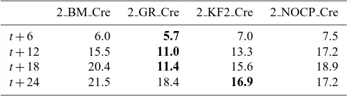
Table 13. Mean Absolute Error (MAE) (mm) for the 9
Novem-ber 2009.
2 BM Cre 2 GR Cre 2 KF2 Cre 2 NOCP Cre
t+6 6.0 5.7 7.0 7.5
t+12 15.5 11.0 13.3 17.2
t+18 20.4 11.4 15.6 18.9
t+24 21.5 18.4 16.9 17.2
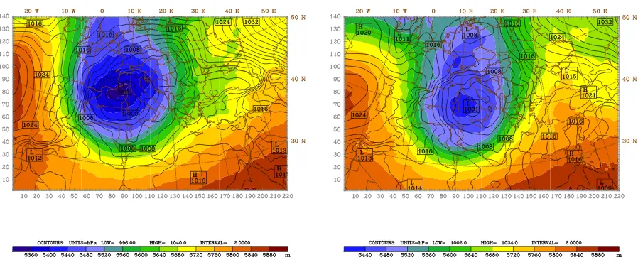
southerly near the surface. This flow, transfers warm and hu-mid air masses from the Ionian Sea over Epirus, and because of the convergence in the direction of motion and the uplift due to the complex topography, creates large precipitation amounts.
Similarly to the above process, MAE (Cressman method) is estimated for the three CPSs as well as for the NOCP simulation. For a more detailed examination of the case, the analysis is carried out for the four 6-h intervals of this day. For each 6-h interval, at least half of the operating rain gauges recorded precipitation exceeding 10 mm, with the highest amounts observed during the last 6-h interval, ex-ceeding 25 mm in most stations. The results for the 2 km
grid are shown in Table 13. It is seen that a CPS is neces-sary with Grell and Kain-Fritsch-2, giving the lowest MAEs. These one-day findings are in agreement with the results for the 22 days.
In order to outline the differentiations between the applica-tion of Kain-Fritsch-2 and NOCP in the finest grid, the corre-sponding distributions of the precipitation heights predicted above Epirus are drawn for each of the 6-h intervals (Fig. 5). In the same figure, the observed precipitation values are plot-ted. As it can be seen, there are areas, mainly coastal and low-land, where Kain-Fritsch-2 predicts light-moderate pre-cipitation (1–10 mm) while NOCP predicts no prepre-cipitation at all.
Fig. 4.
Sea level pressure (hPa) and 500 hPa height (gpdm) for 00:00 and 24:00 UTC of 9 November
2009.
Fig. 4. Sea level pressure (hPa) and 500 hPa height (gpdm) for 00:00 and 24:00 UTC of 9 November 2009.
5 Conclusions
The purpose of this work was to assess the performance of the numerical weather prediction model MM5 over Epirus Region, NW Greece, focusing on the precipitation forecasts. The analysis is based on the results of the simulations of 22 days with intense rainfall over the area of interest. This work was motivated by the fact that MM5 model is used op-erationally at the University of Ioannina with the aim to pro-vide weather forecasts in the area, and it is also the basis of the early warning system developed in the area in the frame of RISKMED project. Three main questions are discussed: (a) does increased resolution grid produce more skilful pre-cipitation forecasts? (b) is the activation of a convective parameterization scheme (CPS) needed at the resolution of 2 km? and (c) which CPS results in the most accurate precip-itation forecasts in the study area? For this reason, three well known CPSs (Betts-Miller, Grell and Kain-Fritsch-2) were utilized for three nested domains with grid resolution of 24, 8 and 2 km. The validation of the model was done for various precipitation classes and thresholds by estimating the Mean Absolute Error and three categorical statistics (Bias, Propor-tion Correct and Equitable Threat score) derived from con-tingency tables. Thereinafter, these validations were also ap-plied for three sub-areas of Epirus, coastal, inland and moun-tainous and finally, a case study was analytically examined.
According to the results,
– An improvement in precipitation prediction appears as horizontal resolution gets higher (from 8 to 2 km). Nev-ertheless, the best results are found if a slight displace-ment (up to 2.8 km) in spatial distribution of rainfall is considered acceptable. The complexity of the terrain of Epirus may be responsible for this.
– In general, the model underestimates precipitation for all three examined CPSs, but the activation of a CPS in the finest grid of 2 km appears necessary as the results are considerably improved; except for mountainous ar-eas where results with or without CPS are comparable. – The CPSs forecasting the most reliable precipitation
heights are Grell and Kain-Fritsch-2, with the former being better for high thresholds (strong precipitation events only) and the latter for small and medium ones (all precipitation events).
– All the examined CPSs give the smallest precipitation errors in the inland sub-area.
For the future, it is planned to extend the present research to further sensitivity experiments, i.e. to examine the role of various microphysical schemes in combination with the three CPSs as well as the role of topography in precipitation dis-tribution in small sub-areas of Epirus. This will be better achieved as more meteorological stations are planned to be installed all over Epirus.
Acknowledgements. The research work is co-funded by the Euro-pean Union – EuroEuro-pean Social Fund (ESF) & National Sources, in the framework of the program “HERAKLEITOS II” of the “Opera-tional Program Education and Life Long Learning” of the Hellenic Ministry of Education, Life Long Learning and religious affairs.
The authors would like to thank the anonymous referees for their valuable suggestions which led to a substantial improvement of the manuscript.
Edited by: A. Mugnai
Fig. 5. Precipitation distribution for each 6-h interval (00:00–06:00, 06:00–12:00, 12:00–18:00, 18:00–24:00 UTC) of 9 November 2009
References
Accadia, C., Mariani, S., Casaioli, M., Lavagnini, A., and Speranza, A.: Sensitivity of precipitation forecast skill scores to bilinear interpolation and a simple nearest-neighbor average method on high-resolution verification grids, Weather Forecast., 18, 918– 932, 2003.
Akylas, E., Kotroni, V., and Lagouvardos, K.: Sensitivity of high resolution operational weather forecasts to the choice of the plan-etary boundary layer scheme, Atmos. Res., 84, 49–57, 2007. Alpert, P., Neeman, B. U., and Shay-El, Y.: Intermonthly variability
of cyclone tracks in the Mediterranean, J. Climate, 3, 1474–1478, 1990.
Anthes, R. A.: A cumulus parameterization scheme utilizing a one-dimensional cloud model, Mon. Weather Rev., 105, 270–286, 1977.
Arakawa, A. and Schubert, W. H.: Interaction of a cumulus cloud ensemble with the large-scale enironment, Part 1, J. Atmos. Sci., 31, 674–701, 1974.
Bartzokas, A., Azzopardi, J., Bertotti, L., Buzzi, A., Cavaleri, L., Conte, D., Davolio, S., Dietrich, S., Drago, A., Drofa, O., Gkikas, A., Kotroni, V., Lagouvardos, K., Lolis, C. J., Michaelides, S., Miglietta, M., Mugnai, A., Music, S., Niko-laides, K., Porc, F., Savvidou, K., and Tsirogianni, M. I.: The RISKMED project: philosophy, methods and products, Nat. Hazards Earth Syst. Sci., 10, 1393–1401, doi:10.5194/nhess-10-1393-2010, 2010.
Belair, S., Methot, A., Mailhot, J., Bilodeau, B., Patoine, A., Pellerin, G., and Cote, J.: Operational implementation of the Fritsch-Clappell convective scheme in the 24-Km Canadian re-gional model, Weather Forecast., 15, 257–274, 2000.
Betts, A. K. and Miller, M. J.: The Betts–Miller scheme, The Repre-sentation of Cumulus Convection in Numerical Models, Meteor. Monogr., Amer. Meteor. Soc., 46, 107–121, 1993.
Bruintjes, R. T., Clark, T. L. and Hall, W. D.: Interactions between topographic airflow and cloud/precipitation development during the passage of a winter storm in Arizzona, J. Atmos. Sci., 51, 48–67, 1994.
Carbone, R. E., Tuttle, J. D., Ahijevych, D. A., and Trier, S. B.: Influences of predictability associated with warm season precip-itation episodes, J. Atmos. Sci., 59, 2033–2056, 2002.
Cohen, C.: A comparison of Cumulus Parameterizations in Ideal-ized Sea-Breeze Simulations, Mon. Weather Rev., 130, 2554– 2571, 2002.
Colle, B. A. and Mass, C. F.: An observational and modeling study of the interaction of low-level southwesterly flow with the Olympic Mountains during COAST IOP 4, Mon. Weather Rev., 124, 2152–2175, 1996.
Colle, B. A., Westrick, K. J., and Mass, C. F.: Evaluation of MM5 and Eta-10 Prcipitation Forecasts over the Pacific Northwest dur-ing the Cool Season, Weather Forecast., 14, 137–154, 1999. Colle, B. A. and Mass, C. F.: The 5–9 February 1996 flooding event
over the Pacific Northwest: Sensitivity studies and evaluation of the MM5 precipitation forecast, Mon. Weather Rev., 128, 593– 618, 2000.
Cressman, G.: An operational objective analysis system, Mon. Weather Rev., 87, 367–374, 1959.
Davis, B. A. S., Brewer, S., Stevenson, A. C., Guiot, J., and Data Contributors: The temperature of Europe during the Holocene reconstructed prom pollen data, Quat. Sci. Rev., 22, 1701–1716,
2003.
Ducrocq, V., Ricard, D., Lafore, J-P., and Orain, F.: Storm-Scale Numerical Rainfall Prediction for Five Precipitating Events over France: On the Importance of the Initial Humidity Field, Weather Forecast., 17, 1236–1256, 2002.
Dudhia, J.: Numerical study of convection observed during the Winter Monsoon Experiment using a mesoscale two-dimensional model, J. Atmos. Sci., 46, 3077–3107, 1989.
Dudhia, J.: A non-hydrostatic version of the Penn State/NCAR ne-soscale model: validation tests and simulations of an Atlantic cy-clone and cold front, Mon. Weather Rev., 121, 1493–1513, 1993. Emanuel, K. A. and Raymond, D. J.: The representation of Cu-mulus Convection in Numerical Models, Meteor. Monogr., Am. Meteor. Society., 46, 246 pp., 1993.
Federico, S., Avolio, E., Bellecci, C., Colacino, M., Lavagnini, A., Accadia, C., Mariani, S., and Casaioli, M.: Three model inter-comparison for quantitative precipitation forecast over Calabria, Il Nuovo Cimento C, 27, 627–647, 2004.
Ferretti, R., Paolucci, T., Zheng, W., and Visconti, G.: Analyses of the precipitation pattern on the Alpine region using different cumulus convection parameterizations, J. Appl. Meteorol., 39, 182–200, 2000.
Fritsch, J. M. and Chappell, C. F.: Numerical Prediction of Con-vectively Driven Mesoscale Pressure Systems, Part I Convective Parameterization, J. Atmos. Sci., 37, 1722–1733, 1980. Gaudet, B. and Cotton, W. R.: Statistical characteristics of a
real-time precipitation forecasting model, Weather Forecast., 13, 966–982, 1998.
Grell, G. A.: Prognostic evaluation of assumptions used by cumulus parameterizations, Mon. Weather Rev., 121, 764–787, 1993. Grell, G. A., Dudhia, J., and Stauffer, D. R.: A description of
the fifth generation Penn State/NCAR mesoscale model, NCAR Tech. Note NCAR/TN-380+STR, 42 pp., Available from NCAR Information Support Services, P.O. Box 3000, Boulder, CO 80307, 1994.
Hong, S. and Pan, H.: Nonlocal boundary layer vertical diffusion in a medium-range forecast model, Mon. Weather Rev., 124, 2322– 2339, 1996.
Kain, J. S. and Fritsch, J. M.: Convective parameterization for mesoscale models: The Kain-Fritsch scheme, The Represen-tation of Cumulus Convection in Numerical Models, Meteor. Monogr., Amer. Meteor. Soc., 46, 165–170, 1993.
Kain, J. S.: The Kain-Fritsch convective parameterization: An up-date, J. Appl. Meteorol., 43, 170–181, 2004.
Kotroni, V. and Lagouvardos, K.: Precipitation forecast skill of dif-ferent convective parameterization and microphysical schemes: application for the cold season over Greece, Geophys. Res. Lett., 28, 1977–1980, 2001.
Kotroni, V. and Lagouvardos, K.: Evaluation of MM5 highresolu-tion real-time forecasts over the urban area of Athens, Greece, J. Appl. Meteorol., 43, 1666–1678, 2004.
Kuo, H. L.: Further studies on the parameterization of the influence of cumulus convection on large-scale flow, J. Atmos. Sci., 31, 1232–1240, 1974.
Kuo, Y. H., Reed, R. J., and Liu, Y.: The ERICA IOP 5 storm, Part III: Mesoscale cyclogenesis and precipitation parameterization, Mon. Weather Rev., 124, 1409–1434, 1996.
National Observatory of Athens: assessment of two-year oper-ational use, J. Appl. Meteorol., 42, 1667–1678, 2003.
Mazarakis, N., Kotroni, V., Lagouvardos, K., and Argiriou, A. A.: The sensitivity of numerical forecasts to convective parameteri-zation during the warm period and the use of lighting data as an indicator for convective occurrence, Atmos. Res., 94, 704–714, 2009.
Mesinger, F.: Improvements in quantitative precipitation forecasts with the Eta regional model at the National Centers for Environ-mental Prediction: The 48-km upgrade, B. Am. Meteorol. Soc., 77, 2637–2649, 1996.
Nissen, K. M., Leckebusch, G. C., Pinto, J. G., Renggli, D., Ul-brich, S., and UlUl-brich, U.: Cyclones causing wind storms in the Mediterranean: characteristics, trends and links to large-scale patterns, Nat. Hazards Earth Syst. Sci., 10, 1379–1391, doi:10.5194/nhess-10-1379-2010, 2010.
Olson, D. A., Junker, N. W., and Korty, B.: Evaluation of 33 years of quantitative precipitation forecasting at the NMC, Weather Fore-cast., 10, 498–511, 1995.
Schultz, P.: An explicit cloud physics parameterization for oper-ational numerical weather prediction, Mon. Weather Rev., 123, 3331–3343, 1995.
Sindosi, O. A., Batzokas, A., Kotroni, V., and Lagouvardos, K.: A study of MM5 model skill on precipitation over Epirus by us-ing various horizontal resolutions and cumulus parameterization schemes. Proceedings of the 10th Hellenic Conference on Me-teorology, Climatology and Atmospheric Physics, University of Patra, Patra, May 2010, 158–168, 2010 (in Greek).
Trigo, I. F., Bigg, G. R., and Davies, T. D.: Climatology of cyclo-genesis mechanisms in the Mediterranean, Mon. Weather Rev., 130, 549–569, 2002.
Wang, W. and Seaman, N. L.: A comparison study of convective parameterization schemes in a mesoscale model, Mon. Weather Rev., 125, 252–278, 1997.
Weisman, L. M., Klemp, J. B., and Skamarock, W. C.: The reso-lution dependence of explicitly-modeled convection. Preprints, Ninth Conf. on Numerical Weather Prediction, Denver, CO, Amer. Meteor. Soc., 21, 1594–1609, 1991.
Wilson, J. W. and Roberts, R. D.: Summary of Convective storm initiation and during IHOP: observational and modeling perspec-tive, Mon. Weather Rev., 134, 23–47, 2006.