On the Performance Analysis and Evaluation of Scaled Largest Eigenvalue in Spectrum Sensing: A Simple Form Approach

(1)

On the Performance Analysis and Evaluation of

Scaled Largest Eigenvalue in Spectrum Sensing: A

Simple Form Approach

Hussein Kobeissi

1,2,∗

, Amor Nafkha

1

, Youssef Nasser

3

, Oussama Bazzi

2

, Yves Louët

1

1_{SCEE/IETR, CentraleSupélec - Campus de Rennes, Rennes, France.}

2_{Department of Physics and Electronics, Faculty of Science 1, Lebanese University, Beirut, Lebanon.} 3_{ECE Department, AUB, Bliss Street, Beirut, Lebanon.}

Abstract

Scaled Largest Eigenvalue (SLE) detector stands out as the optimal single-primary-user detector in uncertain noisy environments. In this paper, we consider a multi-antenna cognitive radio system in which we aim at detecting the presence/absence of a Primary User (PU) using the SLE detector. By the exploitation of the distributions of the largest eigenvalue and the trace of the receiver sample covariance matrix, we show that the SLE could be modeled using the standard Gaussian function. Moreover, we derive the distribution of the SLE and deduce a simple yet accurate form of the probability of false alarm and the probability of detection.

Hence, this derivation yields a very simple form of the detection threshold. Correlation coefficient between the

largest eigenvalue and the trace is also considered as we derive a simple analytical expression. These analytical derivations are validated through extensive Monte Carlo simulations

Receivedon 01 June 2016;acceptedon 20 February 2017;publishedon 23 February 2017 Keywords: Scaled largest eigenvalue detector, Spectrum sensing, Wishart matrix

Copyright © 2017 H. Kobeissi etal., licensed to EAI. Thisisan open access articledistributedunderthe termsofthe Creative Commons Attribution license (http://creativecommons.org/licenses/by/3.0/), which permits unlimited use,distributionandreproductioninanymediumsolongastheoriginalworkisproperlycited.

doi:10.4108/eai.23-2-2017.152193

1. Introduction

In Cognitive Radio (CR) networks, Spectrum Sensing (SS) is the task of obtaining awareness about the spectrum usage. Mainly it concerns two scenarios of detection: (i) detecting the absence of the Primary User (PU) in a licensed spectrum in order to use it and (ii) detecting the presence of the PU to avoid interference. Hence, SS plays a major role in the performance of the CR as well as the performance of the PU networks that coexist. In this context, an extreme importance for a CR network is to have an optimal SS technique with high probability of accuracy in uncertain environments. The Scaled Largest Eigenvalue detector (SLE) is an efficient technique that is proved to be the optimal detector under Generalized Likelihood Ratio (GLR) criterion and noise uncertainty environments [1,2].

SLE is among the detectors that use the eigenvalues of the receiver sample covariance matrix. Such detectors

∗

Corresponding author. Email:[email protected]

are known as the Eigenvalue Based Detectors (EBD) and include, in addition to SLE [1–7], other detectors like the Largest Eigenvalue detector (LE) and the Standard Condition Number detector (SCN)[8–12]. In a scenario with perfect knowledge of the noise power, the LE detector is the optimal detector [10]. However, in practical systems the noise power may not be perfectly known. In this case, the SLE and SCN detectors outperform the LE detector due to their blind nature. Moreover, the SLE is proved to be the optimal detector under GLR criterion [1, 2] and outperforms the SCN detector.

In literature, results on the statistics of the SLE, defined as the ratio of the largest eigenvalue to the normalized trace of the sample covariance matrix, are relatively limited. They are based on tools from random matrix theory [2–4] and Mellin transform [4– 6]. SLE was proved, asymptotically, to follow the LE distribution (i.e. Tracy-Widom (TW) distribution) [2]. However, a non-negligible error still exists and a new form is derived based on TW distribution and its second

(2)

derivative [3]. Using Mellin transform, The distribution of the SLE was derived by the exploitation of the distribution of LE and the distribution of the trace [4– 6]. However, all the findings on SLE are too complex to be considered in real-environments and hence are no easily scalable. This is due to either a complexity in the original distributions used to model the SLE (e.g. TW distribution) or in the methods used to derive the thresholds. Hence, there is a necessity to propose novel yet simple forms in both SS cases (presence and absence of PU activity).

In this paper, we are interested in finding a simple form for the Cumulative Density Function (CDF) and Probability Density Function (PDF) of the SLE. We consider the following hypotheses: (i) H₀_{: there}

is no primary user and the received signal is only noise; and (ii) H₁_{: the primary user exists. Based}

on the distribution of the ratio of jointly Gaussian random variables, we show that the SLE, under both hypotheses, could be modeled using the standard Gaussian function. Accordingly simple forms for the Probability of False-alarm (Pf a), the Probability of detection (Pd) as well as the detection threshold could be derived. Moreover, we derive the correlation coefficient between the Largest Eigenvalue and the trace in both cases, as it is needed in the derivation of the detection analysis. In the following, we summarize the contributions of this paper:

• Derivation of the distribution of the trace of a complex sample covariance matrix for both H₀

andH₁_hypothesis.

• Derivation of the distribution of the SLE detector for both hypotheses.

• Derivation of a simple form for the correlation coefficient between the largest eigenvalue and the trace under both hypotheses.

• Derivation of a simple form for the probability of false-alarm,Pf a, the detection probability,Pd, and the threshold for detection.

The rest of this paper is organized as follows. Section 2studies the system model. In section3, we recall the distribution of the LE and we derive the distribution of the trace of complex sample covariance matrix. SLE is considered in section 4 as we derive its distribution. The performance probabilities and the threshold are also addressed. In section5, we consider the correlation coefficient between the largest eigenvalue and the trace. Theoretical findings are validated by simulations in section6while the conclusion is drawn in section7.

Notations. Vectors and Matrices are represented, respectively, by lower and upper case boldface. The symbols |_.| _and _tr₍_._{) indicate, respectively, the}

determinant and trace of a matrix while (.)T, and (.)† are the transpose, and Hermitian symbols respectively. In is the n×n identity matrix. Symbols ∼ stands for "distributed as", E[.] for the expected value andk_.k _for

the Frobenius norm.

2. System Model

Consider a multi-antenna cognitive radio system and denote by K the number of received antennas. Let N be the number of samples collected from each antenna, then the received sample from antenna k= 1· · ·_K _at

instantn= 1· · ·_N _{under the two hypotheses is given by}

H₀_: _y_k₍_n_{) =}_η_k₍_n₎_, ₍₁₎

H₁_: _y_k₍_n_{) =}_s₍_n_{) +}_η_k₍_n₎_, ₍₂₎

with ηk(n) is a complex circular white Gaussian noise with zero mean and unknown variance ση2 ands(n) is the received signal sample including the channel effect. After collecting N samples from each antenna, the received signal matrix,Y, is given by:

Y =               

y1(1) y1(2) · · · y1(N)

y2(1) y2(2) · · · y2(N)

..

. ... . .. ...

yK(1) yK(2) · · · yK(N)

              

, (3)

Without loss of generality, we suppose thatK ≤_N _then

the sample covariance matrix is given by W =Y Y†. Denote the eigenvalues ofW byλ1≥λ2≥ · · · ≥λK >0.

H₀ _Analysis. _Under H₀_{, the received samples are}

complex circular white Gaussian noise with zero mean and unknown variance ση2. Consequently, the sample covariance matrix is a central uncorrelated complex Wishart matrix denoted as W ∼ CW_K₍_{N , σ}_η2_I_{K) where}

K is the size of the matrix,N is the number of Degrees of Freedom (DoF), andσ2

ηIKis the correlation matrix.

H₁ _Analysis. _Under H₁_{, we suppose the existence of}

single PU and the channel is constant during sensing time for simplicity. Consequently, the sample covari-ance matrix is a non-central uncorrelated complex Wishart matrix denoted as W ∼ CW_K(_{N , σ}_η2_I_K_,Ω_K)

whereΩKis a rank-1 non-centrality matrix.

Denote the effective correlation matrix by bΣ_K = ση2IK+ΩK/Nand its vector of ordered eigenvalues byσ=

[σ1, σ2,· · ·, σK]T. Accordingly, W, underH1, could be

modeled as a central semi-correlated complex Wishart matrix denoted asW ∼ CW_K(_{N ,}bΣK)[13]. SinceΩ_K is a rank-1 matrix, then bΣ_K belongs to the class of spiked population model with all but one eigenvalue ofbΣ_Kare still equal toσ_η2whileσ1is given by:

σ1=ση2+ω1/N, (4)

2 EAI Endorsed Transactions

on

(3)

whereω1is the only non-zero eigenvalue ofΩK. Denote the channel power byσ_h2and the signal to noise ratio by

r= σs2σh2

ση2 , then it can be easily shown that:

ω1=tr(ΩK) =N Kr. (5)

3. Distributions of the largest eigenvalue and of

the trace

This section considers the distributions of the LE and of the trace under H₀ _and H₁ _{hypothesis. We prove}

that the LE and the trace follow Gaussian distributions for which the means and variances are formulated. Since the SLE does not depend on the noise power, we suppose, in this section, thatση2= 1. Based on results of this section, we derive the distribution of the SLE in the next section.

3.1. Distribution of the LE

Let λ1 be the maximum eigenvalue of the Wishart matrixW. In the following, we give its distribution for

H₀_andH₁_cases.

H₀ _Case. _{Denote the centered and scaled version of}

λ1 of the central uncorrelated Wishart matrix W∼ CW_K(_{N ,}_I_{K) by:}

λ0₁= λ1−a(K, N)

b(K, N) (6)

with a(K, N) and b(K, N), the centering and scaling coefficients respectively, are defined by:

a(K, N) = (

√

K+

√

N)2 (7)

b(K, N) = (

√

K+

√

N)(K−1/2+N−1/2)13 (8)

then, as (K, N)→ ∞_with _K/N →_c∈₍₀_,_1),_λ0

1 follows a Tracy-Widom distribution of order 2 (TW2) [14]. However, it was shown that, for a fixedK and asN → ∞_,_λ₁_{follows a normal distribution [}₁₅_{]. The mean and}

the variance of λ1 could be approximated using TW2 and they are, respectively, given by :

µλ1 =b(K, N)µT W2+a(K, N), (9)

σ2λ1=b

2₍_{K, N}₎_σ2

T W2, (10)

where µT W2=−1.7710868074 and σT W2 2= 0.8131947928 are, respectively, the mean and variance of TW distribution of order 2. This approximation is very efficient and it achieves high accuracy for K as small as 2 [15].

H₁ _Case. _{Denote the centered and scaled version of}

λ1 of the central semi-correlated Wishart matrixW∼

CW_K₍_{N ,}bΣ_K) by:

λ00₁ = λ1p−a2(K, N , σ) b2(K, N , σ)

(11)

with a2(K, N) andb2(K, N), the centering and scaling coefficients respectively, are defined, respectively, by:

a2(K, N , σ) =σ1(N + K

σ1−₁) (12)

b2(K, N , σ) =σ12(N − K

(σ1−₁₎2) (13)

then, as (K, N)→ ∞_with_K/N →_c∈₍₀_,_{1) and}_{r > r}_c₌

1/

√

KN, λ00₁ follows a standard normal distribution (λ00₁ ∼ N₍₀_,_1))[₁₆_{]. Thus,}_λ1 _{follows a normal}

distribu-tion with mean and variance given by (12) and (13) respectively. However, ifr < rc, thenλ1follows the same distribution as in H₀ _{Case [}₁₆_{]. Accordingly, the PU}

signal has no effect on the eigenvalues and could not be detected.

3.2. Distribution of the Trace

As shown earlier, the distribution ofλ1converges to the Gaussian distribution. On the other hand, letT =P

λi be the trace of the Wishart matrixW then the following theorem holds:

Theorem 1.LetT be the trace of W∼ CW_K₍_{N ,}Σ_{) where}

the vector of eigenvalues ofΣ, not necessary equal, are given by [σ1, σ2,· · · , σK]. Then, as N → ∞, T follows Gaussian distribution as follows:

P(T −N PK

i=1σi q

NPK i=1σi2

≤_x_{) =} √1

2π Zx

−∞

e−u

2

2 _du, ₍₁₄₎

Proof. LetDbe an orthogonal matrix that diagonalizes Σ, then we write:

T =tr(Y Y†) =tr(DDTY Y†) =tr(DTY Y†D)

=tr(Z Z†) = K X

i=1        

N X

j=1

|_z_i,j|2

       

(15)

with zi,j is the (i, j)-th element of matrix Z =DTY. Let Z = [z1 z2· · ·zN] with zj = [z1j z2j· · ·zKj]T. Since the vectors z1,z2,· · ·_z_N _{are independent and} _z_j ∼ CN_K₍₀_,_DT_Σ_D_{) then the elements}_z_ij _{are independent}

and form a circularly symmetric complex normal random variable (zi,j∼ CN(0, σi)). Accordingly, the square of the norm,|_z_i,j|2_{, is exponentially distributed} with parameterσ_i−1 and hence, the mean and variance areσiandσi2respectively.

According to CLT, asN → ∞_{the term in the square}

bracket of (15) follows Gaussian distribution with mean and variance areN σi andN σi2respectively.

To the best of the authors’ knowledge, the result in Theorem1is new.

(4)

H₀_Case. _{The distribution of the trace}_T _{of of}_W _under

H₀_{is given by the following Corollary:}

Corollary 1.Let T be the trace of W∼ CW_K₍_{N , σ}_η2_I_K_).

Then, as N → ∞_, _T _{follows Gaussian distribution as}

follows:

P(T

−_{N Kσ}_η2

q N Kση4

≤_x_{) =}√1

2π Zx

−∞

e−u

2

2_du, ₍₁₆₎

Proof. It follows from Theorem1.

H₁_Case. _{The distribution of the trace}_T _{of of}_W _under

H₁_{is given by the following Corollary:}

Corollary 2.LetT be the trace ofW∼ CW_K₍_{N ,}bΣ_K). Then, asN → ∞_,_T _{follows Gaussian distribution as follows:}

P(Tq−N(σ1+ (K−1)σ2) N(σ₁2+ (K−₁₎_σ2

2)

≤_x_{) =} √1

2π Zx

−∞

e−u

2 2 _du,

(17)

Proof. All the eigenvalues ofbΣ_K are equal except σ1. Then, the result follows from Theorem1.

Normalized Trace. LetTn= K1T be the normalized trace. ThenTn, following Theorem1, is Normally distributed. From Corollary 1, Tn is Normally distributed with mean and variance given respectively, whenση2= 1, by:

µTn =N , (18)

σ2Tn =N /K, (19)

From Corollary 2, Tn is Normally distributed with mean and variance given respectively, whenση2= 1, by:

µTn =

N

K(σ1+K−1), (20)

σ2T_n = N K2(σ

2

1 +K−1), (21)

4. SLE Detector

Let W be the sample covariance matrix at the CR receiver, then the SLE ofW is defined by:

X= ₁ λ1 K

PK i=1λi

= λ1 Tn

(22)

Denoting by α the decision threshold, then the false alarm probability (Pf a), defined as the probability of detecting the presence of PU while it does not exist, and the detection probability (Pd), defined as the probability of correctly detecting the presence of PU, are, respectively, given by:

Pf a=P(X≥α/H0) = 1−F0(α), (23)

Pd =P(X≥α/H1) = 1−F1(α), (24)

whereF0(.) andF1(.) are the CDFs of X underH₀ _and H₁ _{hypotheses respectively. If the expressions of the}

Pf a and/or Pd are known, then a threshold could be set according to a required error constraint. Hence, it is important to have a simple and accurate form for the distribution ofX.

4.1. SLE distribution

This section provides a new formulation for the SLE distribution forH₀_andH₁_{hypotheses as follows:}

H₀ _Case. _Under H₀_{, both the LE and the normalized}

trace follow the Gaussian distribution asN → ∞_which

is realistic in practical spectrum sensing scenarios. Herein, we show that the SLE could be formulated using standard Gaussian function as stated by the following theorem:

Theorem 2.Let X be the SLE of W∼ CW_K₍_{N , σ}_η2_I_K_).

Then, for a fixed K and as N → ∞_{, the CDF and the}

PDF ofXare, respectively, given by:

FX(x) =Φ(

xµTn−µλ1

q σ2

λ1−2xc+x2σ2Tn

) (25)

fX(x) = µTnσ

2

λ1−cµλ1+ (µλ1σ

2

Tn−cµTn)x

(σ2

λ1−2xc+x2σ2Tn)

3 2

× _φ₍ xµTn−µλ1

q σ2

λ1−2xc+x2σ2Tn

) (26)

with

Φ(v) =

Zv

−∞

φ(u)du and φ(u) =√1

2πe

−u2

2 ₍₂₇₎

where µλ1, µTn and σ

2 λ1, σ

2

Tn are, respectively, the

mean and the variance of λ1 andTn given by (9), (18) and (10), (19) respectively. The parameter c is given by c=σλ1σTnρ where ρ is the correlation coefficient

betweenλ1andTn.

Proof. Let λ1 and Tn be two normally distributed random variables with µλ1, µTn, σ

2

λ1 and σ

2

Tn their

means and variances and let ρ be their correlation coefficient. Denote byg(λ, t) the joint density ofλ1and Tn then the PDF ofXisfX(x) =

R+∞

−∞ |t|g(xt, t)dtand the result is found in [17], however, since W is positive definite thenP r(Tn>0) = 1 and the CDF ofXcould be written as:

FX(x) =P r(λ/t < x) =P r(λ1−xt <0) (28)

and thus, its CDF is given by (25) and the PDF is its derivative in (26) [18].

4 EAI Endorsed Transactions

on

(5)

H₁ _Case. _Under H₁_{, the normalized trace follows}

the Gaussian distribution as N → ∞ _{whereas the LE}

follows the Gaussian distribution as (K, N)→ ∞ _with

K/N →_c∈₍₀_,_{1) and}_{r > r}_c_{= 1}_/ √

KN. Accordingly, the distribution of the SLE is given by the following Theorem:

Theorem 3.Let X be the SLE of W∼ CW_K₍_{N ,}bΣ_K). Then, as (K, N)→ ∞_with_K/N →_c∈₍₀_,_{1) and}_{r > r}_c₌

1/

√

KN, the CDF and PDF ofXare, respectively, given by (25) and (26). However, µλ1, µTn and σ

2 λ1, σ

2 Tn

are, respectively, the mean and the variance ofλ1 and Tn given by (12), (20) and (13), (21) respectively. The parameter c is defined by c=σλ1σTnρ where ρ is the

correlation coefficient betweenλ1andTn.

Proof. Same as the proof of Theorem2.

4.2. Performance Probabilities and Threshold

Using (23) and (25), thenPf ais given by:

Pf a(α) =Q( αµTn−µλ1

q σ2

λ1−2αc+α2σ2Tn

) (29)

where Q(.) is the Q-function. µλ1,σ

2

λ1, µTn and σ

2 Tn

are given respectively by (9), (10), (18) and (19).Pd is derived the same way usingH₁_hypothesis.

UsingPf aandPd, the threshold could be set according to a required error constraint. For example, and based on (29), we can derive a simple and accurate form for the threshold as a function of the means and variances of theLEandTnand the correlation coefficient between them as well as the false alarm probability. That is, for a target false alarm probability, ˆPf a, the equation of the threshold of the SLE detector will be:

α=

µ12−β2ρσ12+β q

mv−2ρµ12σ12+β2σ122 (ρ2−1)

µ2_T

n −_β2_σ2

T_n

(30) whereµ12 =µλ1µTn,σ12 =σλ1σTn,mv =µ

2 Tnσ

2

λ₁+µ2λ₁σT2n

andβ=Q−1( ˆPf a) withQ −₁

(.) is the inverse Q-function.

5. Correlation Coefficient

ρ

Theorem2gives the form of the distribution of the SLE as a function of the mean and the variance ofλ1andTn as well as the correlation coefficient between them (ρ). Consequently,Pf a,Pdand the threshold are a functions of these same parameters.

The mean and the variance ofλ1andTnare provided in Section 3. In this section, we will give a simple analytical form to calculate the correlation coefficient, ρ, between the largest eigenvalue and the trace of Wishart matrix based on the mean of the SLE. In the following, we calculate the mean of SLE in two different ways such that a simple form forρcould be derived.

5.1. Mean of SLE using

λ

1

and

T

n

Under both hypotheses (H₀ _and H₁_{), the mean of the}

SLE could be computed using the means ofλ1andTnas follows:

H₀ _{case: using independent property.} _UnderH₀_{, the SLE}

and the trace of central uncorrelated Wishart matrices are proved to be independent [19]. Accordingly, and using (22), the mean ofλ1could be written as:

E[λ1] =EhX×_T_ni₌_E_[_X_]·_E_[_T_n] ₍₃₁₎

Recall that the mean of λ1 and the mean of Tn are given respectively by (9) and (18), then based on (31), the mean of the SLE is given by:

µX = µλ1

µTn

= b(K, N)·µT W2+a(K, N)

N (32)

H₁ _{case: using Taylor series.} _{The bi-variate first order}

Taylor expansion of the function X=g(λ1, Tn) =λ1/Tn about any pointθ= (θλ1, θTn) is written as [20]:

X=g(θ) +g_λ0

1(θ)(λ1−θλ1) +g 0

Tn(θ)(Tn−θTn) +O(n

−₁ ), (33) withg₍0_.₎is the partial derivative ofgover (.).

Letθ= (µλ1, µTn), then the mean is given by [20]:

µX = µλ1

µTn

= σ1(N + K σ1−1) N

K(σ1+K−1)

, (34)

It is worth mentioning that it is more accurate to use higher order Taylor series. However, this will increase the complexity with a slightly more accurate values which is not necessary. Equation (35) provides the expression of the mean using 2ndorder bi-variate Taylor series so that the reader could compare the results.

µX = µλ1

µTn

−Cov(λ1, Tn)

µ2_T

n

+σ 2

Tnµλ1

µ3_T

n

(35)

5.2. Mean of SLE using variable transformation

Using SLE distribution, it is difficult to find numerically the mean of the SLE, however, it turns out that a simple and accurate approximation could be found.

An approximation of the mean of the ratio (u+ Z1)/(v+Z2) could be found whenuandv are positive constants andZ1andZ2are two independent standard normal random variables. It is based on approximating formula forE[1/(v+Z2)] whenv+Z2is normal variate conditioned by Z2>−4 and v+Z2 is not expected to approach zero as follows [18]:

E "

1 v+Z2

#

= 1

(6)

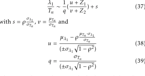
By using the transformation of the general ratio of two jointly normal random variableλ1/Tninto the ratio (u+Z1)/(v+Z2), which has the same distribution, we have:

λ1 Tn

∼ 1

q( u+Z1 v+Z2

) +s (37)

withs=ρσλ1 σ_Tn,v =

µ_Tn σ_Tn and

u= µλ1

−_ρµTn·σλ1 σ_Tn

(±_σ_λ

1

p

1−_ρ2₎ (38)

q= σTn

(±_σ_λ

1

p

1−_ρ2₎ (39)

where one chooses the±_{sign (in both}_u_and_q_{) so that}_u

andv have the same sign (i.e. positive). As the left-side and the right-side of (37) must have the same mean, we can write:

E[λ1 Tn

] = u qE[

1 v+Z2

] +s (40)

therefore the mean of the SLE could be approximated as follows:

µX =

µλ1+δ µTn

θ +δ (41)

withδ=ρσλ1

σ_Tn andθ= 1.01µTn−0.2713σTn.

This practical approximation shows high accuracy; however, it could be noticed from (40) that as u increases the error due to this approximation increases.

5.3. Deduction of the Correlation coefficient

ρ

Based on these results, the correlation coefficient (ρ) underH₀_andH₁_{hypotheses is considered as follows:}

H₀ _case. _{Using (}₄₁_{), then} _ρ_{, after some algebraic}

manipulation, is given by:

ρ= σTn

σλ1

·θ µX

−_µ_λ

1

θ+µTn

(42)

whereµλ1,µTnandµX are respectively the means of the

LE, the normalized trace and the SLE given by (9), (18) and (32) respectively. σλ1 andσTn are respectively the

standard deviations of the LE and the normalized trace and are the square root of (10) and (19) respectively.

H₁ _case. _Under H₁ _{hypothesis, results show the} _u

increases as K or N increases because of the high correlation between λ1 and Tn. Accordingly, results show a small error in the value of the mean of SLE with respect to the true value. Consequently, and using (41), thenρis given by:

ρ= σTn

σλ1

·θ(µX+)

−_µ_λ

1

θ+µTn

(43)

whereµλ1,µTnandµX are respectively the means of the

LE, the normalized trace and the SLE given by (12), (20)

Table 1. The Empirical and Approximated value of the correlation

coefficientρ underH₀ _{hypothesis for different values of}{_{K, N}}_.

K×_N ₂×_{500 4}×_{500 2}×_{1000 4}×_{1000 50}×₁₀₀₀

ρ-Emp. 0.849 0.6974 0.839 0.6915 0.3353 ρ-Ana. 0.8548 0.6957 0.8623 0.6967 0.3356

and (34) respectively. σλ1 and σTn are respectively the

standard deviations of the LE and the normalized trace and are the square root of (13) and (21) respectively. Finally,is a variable used to model the mean error.

6. Numerical validation

In this section, we discuss the analytical results through Monte-Carlo simulations. We validate the theoretical analysis presented in sections 3, 4 and 5. The simulation results are obtained by generating 105 random realizations ofY.

Table 1 shows the accuracy of the analytical approximation of the correlation coefficient (ρ) of the SLE in (42). The results are shown for K ={₂_,₄_,₅₀}

antennas and N ={₅₀₀_,₁₀₀₀} _{samples per antenna.}

Table1shows that the accuracy of this approximation is higher as the number of antennas increases, however, we can also notice that we have very high accuracy even when K = 2 antennas. Also, as expected, it is easy to notice that the correlation between the largest eigenvalue and the trace decreases as the number of antenna increases, however, this correlation could not be ignored even if the number of antennas is large.

Figure 1 shows the accuracy of the mean of the SLE as well as the correlation coefficient between the largest eigenvalue and the trace. The results are shown for different values of K where N = 500 and r=−₁₀_dB_{. Figure}_1(a)_{plots the empirical mean and its}

corresponding Taylor series approximation in (34). In addition, the figure shows the mean error () between the Taylor approximation and the mean expression provided using variable transformation in (41). the results show a high accuracy in the approximation of the mean using Taylor series, however, it also shows a small error, , that increases as K increases. Another important point here concerns the error value epsilon. Indeed, one can easily observe the epsilon is small however its effect on correlation coefficient rho is relatively high as shown in Fig.1(b), hence corrective action should be taken to yield correct results. The corrected version is considered (i.e. Fig.1(a)) then the results show high accuracy. We should mention that this is out of the scope of this paper but it is worth mentioning it for future research.

6

EAI Endorsed Transactions on

(7)

0 10 20 30 40 50 60 70 80 90 100 10−4

10−3 10−2 10−1 100 101 102

K

µSLE: Empirical

µ_SLE: Taylor

µ_SLE error (ε)

(a) Empirical and proposed approximation of µSLE with the

corresponding error ()

0 10 20 30 40 50 60 70 80 90 100

0.1 0.2 0.3 0.4 0.5 0.6 0.7 0.8

K

ρ

ρ: Empirical

ρ: Before correction

ρ: After correction

(b) Empiricalρand its corresponding analytical approximation before and after mean correction

Figure 1. Empirical and Analytical mean of SLE (µSLE) and

correlation coefficient between largest eigenvalue and trace (ρ) under H₁ _{hypothesis for different values of} _K _where_N _{= 500}

sample andr=−₁₀_dB_.

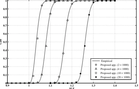
0.9 1 1.1 1.2 1.3 1.4 1.5

0 0.1 0.2 0.3 0.4 0.5 0.6 0.7 0.8 0.9 1

SLE

CDF

Empirical Proposed app. (2 × 1000) Proposed app. (4 × 1000) Proposed app. (10 × 1000) Proposed app. (20 × 1000)

Figure 2. Empirical CDF of the SLE underH₀ _{hypothesis and}

its corresponding Gaussian approximation for different values of

K withN = 1000.

4.5 5 5.5 6 6.5 7

0 0.1 0.2 0.3 0.4 0.5 0.6 0.7 0.8 0.9 1

SLE

CDF

Empirical (50 × 500)

Proposed before correction (50 × 500) Proposed after correction (50 × 500) Empirical (50 × 1000)

Proposed before correction (50 × 1000) Proposed after correction (50 × 1000)

Figure 3. Empirical CDF of the SLE underH₁ _{hypothesis and}

its corresponding proposed approximation for different values of

K = 50withN ={₅₀₀_,₁₀₀}_and_r₌−₁₀_dB_.

0.9 1 1.1 1.2 1.3 1.4 1.5 1.6 1.7 1.8 0

0.1 0.2 0.3 0.4 0.5 0.6 0.7 0.8 0.9 1

Threshold (α) Pfa

Empirical Proposed (2 × 500) Proposed (10 × 500) Proposed (50 × 500)

Figure 4. Empirical probability of false alarm for the SLE

detector and its corresponding proposed form in (29) for different values ofK with N = 500 samples.

Figure 2 shows the empirical CDF of the SLE and its corresponding approximation underH₀ _hypothesis

given by Theorem 2. The results are shown for K ={₂_,₄_,₁₀_,₂₀} _{antennas and} _N _{= 1000 samples per}

antenna. Results show a perfect match between the empirical results and our Gaussian formulation.

Figure 3 shows the empirical CDF of the SLE and its corresponding approximation (before and after mean correction) given by Theorem 3. The results are shown for K = 50 antennas, N ={₅₀₀_,₁₀₀₀} _samples

per antenna and r=−₁₀_dB_{. Again, the results show a}

perfect match between the empirical results and the proposed approximation after the mean correction in (43). However if the we consider= 0, results show a slight difference between empirical and the proposed distributions in comparison with the big error inρ(see Fig.1(b)whenK = 50 andN = 500).

(8)

multi-antenna CR with different number of antennas and N = 500 samples. The considered number of antennas is as small as K = 2 and as large as K = 50. Simulation results show a high accuracy in our proposed form which increases as K increases. It is worth reminding the reader, that in addition to the accuracy, the form given in (29) is a simple Q-function equation.

7. Conclusion

In this paper, we have considered the SLE detector due to its optimal performance in uncertain environments. We proved that the SLE could be modeled using standard Gaussian function and we have derived its CDF and PDF. The false alarm probability, the detection probability and the threshold were also considered as we derived new simple and accurate forms. These forms are simple functions of the means and variances of the LE and the trace as well as the correlation function between them. The correlation between the largest eigenvalue and the trace is studied and simple expressions are provided. Simulation results have shown that the proposed simple forms achieve high accuracy. However, the approximation of the correlation coefficient under H₀ _{shows high accuracy.}

Moreover, underH₁_{hypothesis, small mean error must}

be corrected to achieve high accuracy. In addition, results have shown that the correlation between the largest eigenvalue and the trace, under H₀_{, decreases}

as the number of antenna increases but it could not be ignored even for large number of antennas.

Acknowledgment. This work was funded by a program of cooperation between the Lebanese University and the Azem & Saada social foundation (LU-AZM) and by CentraleSupélec (France).

References

[1] Wang, P., Fang, J., Han, N. and Li, H. (2010)

Multiantenna-assisted spectrum sensing for cognitive radio.Vehicular Technology, IEEE Transactions on59(4): 1791–1800. doi:10.1109/TVT.2009.2037912.

[2] Bianchi, P., Debbah, M., Maida, M. and Najim, J.

(2011) Performance of statistical tests for single-source detection using random matrix theory. IEEE Trans. Inform. Theory, 57(4): 2400–2419. doi:10.1109/TIT.2011.2111710.

[3] Nadler, B. (2011) On the distribution of the ratio of

the largest eigenvalue to the trace of a wishart matrix. Journal of Multivariate Analysis 102(2): 363 – 371. doi:http://dx.doi.org/10.1016/j.jmva.2010.10.005, URL

http://www.sciencedirect.com/science/article/ pii/S0047259X10002113.

[4] Wei, L. and Tirkkonen, O. (2011) Analysis of scaled

largest eigenvalue based detection for spectrum sensing. In Communications (ICC), 2011 IEEE International Conference on: 1–5. doi:10.1109/icc.2011.5962520.

[5] Wei, L., Tirkkonen, O., Dharmawansa, K.D.P. and McKay, M.R. (2012) On the exact distribution of the

scaled largest eigenvalue. CoRR abs/1202.0754. URL

http://arxiv.org/abs/1202.0754.

[6] Wei, L.(2012) Non-asymptotic analysis of scaled largest

eigenvalue based spectrum sensing. In Ultra Modern Telecommunications and Control Systems and Workshops (ICUMT), 2012 4th International Congress on: 955–958. doi:10.1109/ICUMT.2012.6459797.

[7] Kobeissi, H., Nasser, Y., Nafkha, A., Bazzi, O.

and Louët, Y. (2016) A simple formulation for the

distribution of the scaled largest eigenvalue and application to spectrum sensing. In Cognitive Radio Oriented Wireless Networks,172: 284–293.

[8] Cardoso, L.,Debbah, M.,Bianchi, P.andNajim, J.(2008)

Cooperative spectrum sensing using random matrix theory. In in Proc. IEEE Int. Symp. Wireless Pervasive Comput. (ISWPC)(Greece): 334–338.

[9] Zeng, Y. and Liang, Y.C. (2009) Eigenvalue-based

spectrum sensing algorithms for cognitive radio. IEEE Trans. Commun.57(6): 1784–1793.

[10] Nadler, B., Penna, F. and Garello, R. (2011)

Per-formance of eigenvalue-based signal detectors with known and unknown noise level. In Communications (ICC), 2011 IEEE International Conference on: 1–5. doi:10.1109/icc.2011.5963473.

[11] Zhang, W.,Abreu, G.,Inamori, M.andSanada, Y.(2012)

Spectrum sensing algorithms via finite random matrices. IEEE Trans. Commun.60(1): 164–175.

[12] Kobeissi, H., Nasser, Y., Bazzi, O., Louet, Y. and Nafkha, A. (2014) On the performance evaluation

of eigenvalue-based spectrum sensing detector for mimo systems. In XXXIth URSI General Assembly and Scientific Symposium (URSI GASS),: 1–4. doi:10.1109/URSIGASS.2014.6929235.

[13] Tan, W.Y. and Gupta, R.P. (1983) On approximating

the non-central wishart distribution with wishart distribution.Commun. Stat. Theory Method12(22): 2589– 2600.

[14] Johansson, K. (2000) Shape fluctuations and random

matrices.Comm. Math. Phys.209(2): 437–476.

[15] Tirkkonen, O.andWei, L.(2012)Foundation of Cognitive Radio Systems (InTech), chap. Exact and Asymptotic Analysis of Largest Eigenvalue Based Spectrum Sensing, 3–22.

[16] Baik, J., Ben Arous, G. and Péché, S. (2005) Phase

transition of the largest eigenvalue for nonnull complex sample covariance matrices. Ann. Probab.33(5): 1643– 1697. doi:10.1214/009117905000000233, URLhttp:// dx.doi.org/10.1214/009117905000000233.

[17] Hinkley, D.V. (1969) On the ratio of two correlated

normal random variables.Biometrika56(3): 635–639. [18] Marsaglia, G.(2006) Ratios of normal variables.Journal

of Statistical Software16(4): 1–10.

[19] Besson, O.andScharf, L.(2006) Cfar matched direction

detector. Signal Processing, IEEE Transactions on54(7): 2840–2844. doi:10.1109/TSP.2006.874782.

[20] Kobeissi, H., Nafkha, A., Nasser, Y., Bazzi, O. and Louët, Y. (2016) Simple and accurate closed-form

approximation of the standard condition number distribution with application in spectrum sensing. In

CROWNCOM.

8

EAI Endorsed Transactions on