The M/G/1 queueing model with preemptive random
priorities
Moshe Haviv
Department of Statistics and the Federmann Center for the Study of Rationality
The Hebrew University of Jerusalem
91905 Jerusalem
Israel
[email protected]
ABSTRACT
For the M/G/1 model, we look into a preemptive prior-ity scheme in which the priorprior-ity level is decided by a lot-tery. Such a scheme has no effect on the mean waiting time in the non-preemptive case (in comparison with the First Come First Served (FCFS) regime, for example). This is not the case when priority comes with preemption. We derived the resulting mean waiting time (which is invari-ant with respect to the lottery performed) and show that it lies between the corresponding means under the FCFS and the Last Come First Served with Preemption Resume (LCFS-PR) (or equivalently, the Egalitarian Processor Shar-ing (EPS)) schemes. We also derive an expression for the Laplace-Stieltjes transform for the time in the system in this model. Finally, we show how this priority scheme may lead to an improvement in the utilization of the server when cus-tomer decide whether or not to join.
Categories and Subject Descriptors
G.3 [Probability and Statistics]: Queueing theory, Stochas-tic Processes
Keywords
priority queues,preemption,performance evaluation
1.
INTRODUCTION
The M/G/1 queueing model is one of the most researched model in operations research and in the performance eval-uation area of computer sciences. In this model customers arrive to a single server queue with accordance to a Pois-son process with rate denoted byλper unit of time. Ser-vice times are independent and identically distributed with cumulative distribution function G. Denote by G∗(s) the Laplace-Stieltjes transform (LST) of the service time, namely
G∗(s) = E(e−sX) whereX≥0 is a random variable repre-senting a single service time. This distribution is not limited to belong to any specific family of distributions (such as the
exponential family). Denote byxandx2 the first and sec-ond moments of service times, respectively. We denote λx byρand assume for stability thatρ <1. It is well-known thatρis the server utilization level, namely the proportion of time where the server is busy.
There are various possible service regimes. The most known one is First Come First Served (FCFS). Under this regime the mean waiting time in the system (queueing plus service), denoted by E(WF CF S), equals
E(WF CF S) = λx2
2(1−ρ)+x. (1)
This is the well-known Khintchine-Pollaczek formula, which is apparently the most important queueing result. See, e.g., [6], p.60. It is well-known (and easily argued by Little’s rule) that this value for the mean waiting time does not vary with the service regime as long as preemption (i.e., interrupting service during its execution) is not allowed and as long as non-anticipation (i.e., order of service is not based on prior knowledge of the actual service times) is assumed.
Two other well-known service regimes are that of Last Come First Served with Preemption Resume (LCFS-PR) and Egal-itarian Processor Sharing (EPS). Under the former regime last to arrive have preemptive priority over those who have arrived earlier. Customers might be preempted while in ser-vice and when they return to serser-vice, it is resumed from the point where is was interrupted last. Under the EPS regime, the server splits its service capacity evenly among all those who are present in the system at any given time instant. This means that ifncustomers are present, they all receive a service of length Δt/nduring a period of length Δt (as-suming Δtis short enough and no change innoccurs). It is well known that under these two schemes the mean time in the system for a customer whose service time equalsx, is
x/(1−ρ). See, e.g., [6], p.63. In particular, the mean time in the system equals
x/(1−ρ). (2)
Since we are concern in this article only with mean values, we next refer only to the LCFS-PR regime but whatever we derive is applicable to the EPS regime as well. In particu-lar, we denote by E(WLCF S−P R) the common mean waiting time.
Which of the two regimes, FCFS or LCFS-PR, is better?
3HUPLVVLRQWRPDNHGLJLWDORUKDUGFRSLHVRIDOORUSDUWRIWKLVZRUNIRU SHUVRQDORUFODVVURRPXVHLVJUDQWHGZLWKRXWIHHSURYLGHGWKDWFRSLHV DUHQRWPDGHRUGLVWULEXWHGIRUSURILWRUFRPPHUFLDODGYDQWDJHDQGWKDW FRSLHVEHDUWKLVQRWLFHDQGWKHIXOOFLWDWLRQRQWKHILUVWSDJH7RFRS\ RWKHUZLVHWRUHSXEOLVKWRSRVWRQVHUYHUVRUWRUHGLVWULEXWHWROLVWV UHTXLUHVSULRUVSHFLILFSHUPLVVLRQDQGRUDIHH
9$/8(722/6'HFHPEHU%UDWLVODYD6ORYDNLD &RS\ULJKWk,&67
'2,LFVWYDOXHWRROV
From the question regarding the mean waiting time the an-swer is clear: Comparing (1) with (2), FCFS comes with a lower mean time in the system, namely 2(1λx−2ρ)+x < 1−xρ,
if and only if CoV(X)<1, where CoV(X) =x2−x2/x. The opposite is the case where CoV(X)>1. They are equal when CoV(X) = 1, which is for example the case where ser-vice times follow exponential distribution.1
Nevertheless, mean time in the system is not necessarily the single criterion to look at. FCFS looks fair and the norm in many cases. It also does not discriminate between customers based on their service requirement (which can be looked at a plus or a minus depending on the eye of the beholder). In particular, long jobs may need to hang around for a long time. Thus, FCFS can be the preferred discipline even when CoV(X)>1, i.e., when it comes with a higher mean waiting time. On the other hand, LCFS-PR and EPS have the theoretical advantage that the mean waiting time exists even in the case where the second moment of service does not exists (or, less formally, whenx2=∞).
We next suggest a queueing regime which can be looked as the ‘middle of the road’: The resulting mean time in the system lies between the corresponding means under the FCFS and LCFS-PR regimes. Thus, in the case where CoV(X)>1, by adopting the suggested scheme, one can do better in terms of reducing the mean sojourn time in com-parison with the FCFS regime, without having to ‘starve’ the long jobs in the same scale as the LFCS-PR or the EPS regimes do.
The regime we define will be called Preemptive Random Pri-ority (PRP). Under this scheme each arrival draws a ran-dom number which is uniformly distributed between zero and one. This number determines his preemptive priority level. We adopt the convention that the lower is the num-ber drown, the higher the priority is. Specifically, one who draws a value ofpis served before one who draws a value of
qwhenp < q, possibly preempting the latter if found in ser-vice upon the arrival of the former. A preempted customer resumes service when his turn (based, again, on his priority parameter) comes, from the point where it was interrupted last. Denote by E(WP RP) the resulting mean time in the system. We show in the next section that E(WP RP) lies between E(WF CF S) and E(WLCF S−P R) (where, of course, the complete order is determined by comparing the service coefficient of variation of X to one). Note that had pre-emption not been allowed, the resulting mean waiting value would coincide with that of FCFS. Also note that since all continuous lotteries are monotone transformations of each other, the assumption of priorities determined by a uniform distribution is without loss of generality.
Remark. Note that in order to operate the PRP regime there is no need to maintain the order in which customers which are currently present had arrived (as is the case of the
1Its easy to see that CoV(X) < 1 (CoV(X) > 1, respec-tively) if and only ifx2/2x < x (x2/2x < x, respectively). This means that the mean residual service time of a cus-tomer who is currently in service is smaller (larger, respec-tively) than the mean service time of a ‘fresh’ customer. For more on this concept see, e.g., [6], Chapter 2.
FCFS and the LCFS-PR regimes) or the order in which they receive service last (as in the case EPS regime when looked as the limit of the round-robin scheme).
We are aware of two references in which the PRP regime is used. These are [2] and [4] (see also [5], pp.102-104). There, PRP is not assumed but rather turned out to be the result-ing regime when customers have the option to pay in order to get a preemptive priority parameter. The more they pay, the higher is their preemptive priority level, reducing their mean waiting costs. In the latter reference, customers have also the option to opt out under a standard cost/reward as-sumption. Minding the trade-off between length of wait and the level of payment, and noticing that other customers face a similar dilemma, their equilibrium behavior is to pay a random amount (having some specific distribution) result-ing overall in the PRP regime. In the latter model some will opt out and, interestingly, in the case of an exponential service time (i.e., anM/M/1 model), the fraction of those who join coincide with the socially optimal joining rate. The
M/M/1 case is also dealt with in [7]. It is shown there that if the regime imposed is that of PRP and customers decide whether or not to join after drawing and inspecting their pri-ority parameters, then the resulting equilibrium joining rate coincides with the socially optimal rate. Finally, the reader is referred to Part VII of [3] for a comprehensive summary on various queueing regimes.
2.
MAIN RESULTS
Theorem 2.1. The mean waiting time in the preemptive random priority (PRP) M/G/1 queue equals
E(WP RP) =ρ+ (1−ρ) ln(1−ρ) (1−ρ)ρ2
λx2 2 −
ln(1−ρ)
ρ x (3)
or, alternatively,
E(WP RP) = 1 1−ρ
x2
2x−
ln(1−ρ)
ρ (x− x2
2x). (4)
In particular, E(WP RP)is bounded between E(WF CF S)and E(WLCF S−P R). Specifically, if CoV(X)<1then
E(WF CF S)<E(WRP R)<E(WLCF S),
where the inequalities are reversed in the case where CoV(X)> 1.
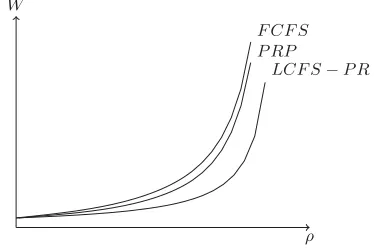
See Figures 1 and 2 below for two examples.
Proof. Denote byPthe random priority level that an ar-bitrary customer draws. Tag a customer and set his priority parameter to p. It means that a mass of size pgets pre-emptive priority over him. Then, by, e.g., [9], p.125, or [6], pp.76-77, his mean time in the system, equals
E(W|P =p) = λp 2(1−pρ)2x2+
1
1−pρx. (5)
Clearly, E(WP RP) = E(E(W|P)). Our proof for (3) and (4) is completed by integrating the right-hand-side of (5) with
respect topfrom p= 0 through p= 1. The second part of the theorem is immediate knowing all three values and using a little bit of algebra.
Clearly, limρ→0E(WP RP) =x and limρ→1E(WP RP) =∞. The following corollary says what is the relative performance of the PRP in comparison with the FCFS and the LCFS-PR regimes under heavy traffic. Its proof is straightforward and hence omitted.
Corollary 2.2.
lim
ρ→1
E(WP RP) E(WLCF S−P R)=
x2
2x
and
lim
ρ→1
E(WP RP) E(WF CF S)= 1.
ρ W
F CF S P RP LCF S−P R
Figure 1: Mean waiting times under the three ser-vice regimes in the casex¯= 1 andCoV(X) = 0as a function ofρ.
ρ W
F CF S P RP
LCF S−P R
Figure 2: Mean waiting times under the three ser-vice regimes in the casex¯= 1 andCoV(X) = 2as a function ofρ.
3.
DISTRIBUTION OF TIME IN THE
SYS-TEM
Before moving on we like to introduce the concept of a stand-by customer. We define a stand-stand-by customer as one who is singled out to receive service only when the system is otherwise empty. In particular, he is always preempted from
service when someone else arrives. Using the terminology of the previous section, he is the one, and only one, who has drawn a priority parameter 1. Likewise, from the point of view of the customers who possesses a priority parameter less than or equal top, the customer with parameterpis a stand-by customer. Note that a stand-by customer does not inflict any extra waiting on any of the other customers. An economist would say here that his decision whether or not to join the queue does not come with anyexternalities.
Our interest in this section is in the LST of the time in the system under the PRP regime. Below we deal first with the M/M/1 case and then with the more general M/G/1 cases. Admittedly, one can derive the former case from the latter but with a minimal cost in space we do the special case first while utilizing its special features and then we switch to the more general case.
3.1
The M/M/1 case
LetB∗(s) denoted the LST of a busy period in an M/M/1 queue. It is well-known that if the arrival rate isλandμis the service rate (recall thatμ−1=x) then (assumingλ < μ)
B∗(s) =λ+μ+s−
(λ+μ+s)2−4λμ
2λ . (6)
See, e.g. [6], p.91.
Lemma 3.1. The LST of the time in the system for a stand-by customer in an M/M/1 queue equals
(1−ρ)B∗(s)
1−ρB∗(s) (7)
whereB∗(s)can be read from (6).
Proof. A customer who sees upon his arrivaln≥0 cus-tomers, has to stay in the system for time which is the sum of
n+ 1 independent and identically distributed busy periods. The (conditional) LST is then (B∗(s))n+1. The probability of seeing this number is (1−ρ)ρn,n≥0. See, e.g.,[6], p.120. Hence, the unconditional LTS equals
∞
n=0
(1−ρ)ρn(B∗(s))n+1=(1−ρ)B ∗(s)
1−ρB∗(s)
as required.
Remark. The mean time in the system for a stand-by cus-tomer is 1/[(1−ρ)2μ] (see [6], p.64), while its variance equals [1 + 2ρ]/[(1−ρ)4μ2]. We omit a detailed proof for the latter fact.
As said, a customer who draws a priority parameter ofp, his time in the system is as that of a stand-by customer in an M/M/1 but with an arrival rate ofλpor, equivalently, with a traffic intensity of pρ. Using (7), we conclude that the LST of his time in the system, denoted next byTp∗(s), equals
Tp∗(s) =
(1−pρ)B∗p(s) 1−pρB∗p(s)
where from (6),
B∗p(s) =λp
+μ+s−(λp+μ+s)2−4λpμ
2λp . (8)
Finally, the corresponding LST of the sojourn time o a ran-dom customer equals
1
p=0T ∗
p(s)dp.
As of now, this is the most explicit expression we were able to derive for the LST of the sojourn time of a random customer in M/M/1 under the PRP regime.
3.2
The M/G/1 case
It is well known that the LST of the time in the system for a customer in a FCFS M/G/1 equals
W∗(s) = (1−ρ) sG ∗(s)
λG∗(s) +s−λ (9) whereG∗(s) is the LST for a single service time. See, e.g., [6], p.86. Note that this is also the LST of the total workload which is held in the system upon arrival instants (as well as at any random instant). We denote byB∗(s) the LST of a standard busy period. There is no explicit expression for this transform (the case of an M/M/1 considered is the previous section (see (6)) is an exception). Yet, it is known thatB∗(s) obeys the condition
B∗(s) =G∗(s+λ(1−B∗(s))). (10) This identity can lead to the finding of all the moments of a busy period. See, e.g., [6], p.92, for the first two. They are
x/(1−ρ) andx2/(1−ρ)3, respectively. Consider now the time in the system of a stand-by customer. We next look for the LST of his time in the system.
Theorem 3.2. Denote byT∗(s)the LST of the time spend in the system by a stand-by customer in an M/G/1 queue. Then,
T∗(s) = (1−ρ)(s+λ(1−B ∗(
s)))B∗(s)
s .
We next give two proofs for this theorem.
Proof. It is possible to see that his time there coincides with a non-standard busy period, namely a busy period whose first service time is different than that of all others (whose distribution is G(x)). Moreover, this first service time is in fact the total work he finds in the system (in-clusive is own) upon his arrival. Note that the LST of this ‘special service’ appears in (9). One can find in the litera-ture the LST of a non-standard busy period. Specifically, denoting byG0(s) the LST of the special service, then the LST of the non-standard busy period equals
G0(s+λ−λB∗(s)).
See, e.g., [6], p.95. All needs to be done now, is to useW∗(s) as given in (9) asG0(s). We can hence conclude, after some algebra (and with the help of (10)) that
T∗(s) = W∗(s+λ−λB∗(s))
= (1−ρ)(λGs+∗λ(−s+λBλ−∗(λBs))∗G(s(s))++λs−−λBλB∗∗((ss))) = (1−ρ)(s+λ(1−B∗s(s)))B∗(s),
(11)
as required.
Proof. In the case where he arrives to an empty system, a probability 1−ρevent, his conditional LST equalsB∗(s). Otherwise, a probability ρevent, he needs to wait for the residual of the running busy period. This comes with a LST of (1−B∗(s))/(sE(B)) where E(B), the mean busy period, which equalsx/(1−ρ). See, e.g., [6], p.30. This needs to be multiplied byB∗(s) due to the busy period which initiates as soon as he enters service for the first and is concluded upon his departure. In summary,
T∗(s) = (1−ρ)B∗(s) +ρ1−B ∗(s)
sx (1−ρ)B ∗(
s). (12)
The rest is algebra.
Theorem 3.3. The mean sojourn time of a stand-by cus-tomer in an M/G/1 queue equals
λx2 2(1−ρ)2+
x
1−ρ. (13)
We next suggest three proofs for this theorem.
Proof. Take the derivative with respect tosin (12) and inserts= 0. The call for the L’Hospital rule will be required. In particular, the second moment of the busy period will be required. It equalsx2/(1−ρ)3(see, e.g. [6], pp.92). We omit any further details.
Proof. Upon arrival, the amount of work found by the stand-by customer (or by any body else) and inclusive of his own, equals
λx2
2(1−ρ)+x. (14) This needs to be divided by 1−ρin order to find the mean time until the system is emptied for the first time (see, e.g. [6], p.63), an instant of time which coincides with the instant in which the stand-by customer departs.
Proof. A third way is to look into the model as one with preemptive priority with two classes. All are in the high priority class, while a single customer (who represents a zero arrival rate class) is inferior. Both classes of course share the same first two moments x andx2. See, e.g.,[9], p.125 or [6], p.76-77, which gives the mean sojourn time for customers of both classes. For the inferior class who has an arrival rate of zero, this means coincides with (13).
Remark. From [8], we learn that the expected marginal externalities that a customer inflicts on others in case of a FCFS regime, equals
λx2 2(1−ρ)2.
To this we need to add his own mean sojourn time, which is stated in (1), in order to find out the total social costs
inflicted by an arrival. As we can see, we do not get the same value that we got for the mean time in the system for a stand-by customer. Yet, the two coincide in case of an ex-ponential service time (something which can be checked with minimal algebra). The reason behind that is that in com-paring systems, one with an extra customer and the other without, under the same arrival and service processes, one gets always one more customer in the former case from one’s arrival until the system is empty for the first time, only if one assumes exponential service times. Hence, the mean time for a stand-by customer and mean added social costs coincide in case of exponential service. This is not the case under a general service distribution.
For a customer who draws a priority level of p, the LST of his time in the system is as above where λis replaced byλp. Specifically, denote this LST byTp∗(s) and conclude from (11) that
Tp∗(s) = (1−pρ)
(s+λp(1−B∗p(s)))Bp∗(s)
s .
where Bp∗(s) is the LST of the busy period but with an arrival rate ofλp, rather than λ.2 Likewise, when we look for the mean value, we need to replace in (13)λwithλpand
ρwithpρ. In particular, the corresponding mean equals
pλx2 2(1−pρ)2 +
x
1−pρ (15)
The following theorem is now immediate.
Theorem 3.4. Denote by TP RP∗ (s) the LST of the so-journ time of a customer in a PRP M/G/1 queue. Then,
TP RP∗ (s) = 1
p=0
(1−pρ)(s+λp(1−B ∗
p(s)))Bp∗(s)
s dp.
As for the mean value, we can by-pass the need to have in hand first the LST. Firstly, it was derived independently in Theorem 2.1. Secondly, we use (15) and derive
E(WP RP) =
1
p=0 ( λpx2
2(1−pρ)2+1−xpρ)dp.
Of course, one should get the same result.
4.
EQUILIBRIUM BEHAVIOR AND SERVER
UTILIZATION
Assume now that customers gain a value ofRdue to service completion and it costs each one of themCper unit of time in the system (service inclusive). Thus,R−CW is the mean net return from joining whenW denotes the mean time in the system. Without loss of generality, we assume that not joining comes with a zero reward (otherwise, one would need to shiftRaccordingly). It would then makes sense to assume that one joins if and only if one’s net gain from joining is positive. ConsiderW now as a function of the arrival rate and denote it hence by W(y) when y is the arrival rate. Assume now thatλ, which as of now will be looked at as thepotentialarrival rate, is such thatR−CW(λ)<0. In 2See (8) for the case of M/M/1.
other words, if all join, one is better off not joining. As-sume also thatR > Cx, namely the reward is larger than the cost of time due just to the time in service. Then, one is better off joining when no-body else does that. We have reached a circular reasoning. The Nash equilibrium concept from non-cooperative game theory deals with such cases. In particular, it implies that each customer should join with a probability ofpewherepesolvesR−CW(λpe) = 0. Indeed, when all join with a probability ofpe, one is indifferent be-tween joining and not, and hence one is willing to randomize between the two options with any probability,peinclusive. For more on this concept in the context of queues, see [1, 5].
Assuming that customers behave in accordance with such an equilibrium behavior is somewhat sad news: Those who join, as well as those who do not join, end up with nothing. Nothing is also the social gain, or the consumer surplus, here. Moreover, changing the functionW (for example, by changing the queue regime or by changing the service rate), does not lead to any individual or social gain. Indeed, for commuters who use a road which is usually jammed, adding another lane will not help: Once this is done, more com-muters will use the road, leading to the same (slow) traffic speed.
The previous paragraph implies that indeed from the cus-tomers point of view it indeed does not matter which queue-ing regime is used. But this is certainly not the case from the point of view of the server (or the one who owns the ser-vice facility). This is the case since the server utilization in equilibrium, which equalsλpex, may vary with the regime due to the simple reason thatpevaries with it.
Theorem 4.1. Denote by pF CF Se the Nash equilibrium joining probability under the queueing regime is FCFS. De-fine pP RPe and pLCF Se −P R in a similar fashion. Then, if CoV(X)<1,
pF CF Se < pP RPe < pLCF Se −P R.
The inequalities are reversed when CoV(X)>1.
The proof of this theorem is now straightforward and we omit the details. An example for a consequence from this theorem is that ifCoV(X)>1 and the current norm is to use FCFS, switching to PRP will decrease the server utiliza-tion (and hence the server might be useful for some other functions) without effecting the social benefit. Of course, one might imagine cases in which one likes to increase the server’s utilization. Hence, such a switch will be recom-mended in the case where CoV(X)<1.
Acknowledgement
Comments made by Yoav Kerner and Binyamin Oz are highly appreciated. The research was supported by an ISF grant no. 1319/11.
5.
REFERENCES
[1] Edleson, N.M. and D.K. Hildebrand (1975), “Congestion tolls for Poisson queueing process,”
Econometrica,43, 81-92.
[2] Glazer, A. and R. Hassin (1986), “Stable prioirity purchasing in queues,”Operations Reserch Letters,4, 285-288.
[3] Harchol-Balter, M. (2013),Performance Modeling and Design of Computer Systems: Queueing Theory in Action, Cambridge University Press, Cambridge. [4] Hassin, R. (1995), “Decentralized regulation of a
queue,”Management Science,41, 163-173.
[5] Hassin, R. and M. Haviv (2003),To Queue or not to Queue: Equilibrium Behaviour in Queueing Systems, Kluwer.
[6] Haviv, M. (2013),Queueus - A Course in Queueing Theorey, Springer.
[7] Haviv, M. and B. Oz (2014), “Self-regulation in a queue via random priorities,” (in preparation). [8] Haviv, M. and Y. Ritov (1998), “Externalities, tangible externalities and queue disciplines,” Management Science,44, 850-858.
[9] Kleinrock, L. (1976)Queueing systems, Volume 2: Computer applications, John Wiley and Sons, New York.