A Performance Perspective on Choosing between Single Aggregate and Multiple Aggregates for GENI Experime nts

(1)

A

Performance

Perspective

on

Choosing

between

Single

Aggregate and Multiple Aggregates for GENI Experiments

Zongming Fei

1,∗

_{, Ping Yi}

1

_{, Jianjun Yang}

2

1_{Department of Computer Science, University of Kentucky, Lexington, KY 40506, USA} 2_{Department of Computer Science, University of North Georgia, Oakwood, GA 30566, USA}

Abstract

TheGlobalEnvironmentforNetworkInnovations(GENI)providesavirtuallaboratoryforexploringfutureinternetsat scale.Itconsistsofmanygeographicallydistributedaggregatesforprovidingcomputingandnetworkingresourcesfor settingupnetworkexperiments.AkeydesignquestionforGENIexperimentersiswheretheyshouldreservetheresources, andinparticularwhethertheyshouldreservetheresourcesfromasingleaggregateorfrommultipleaggregates.Thisnot onlydependsonthenatureoftheexperiment,butneedsabetterunderstandingofunderlyingGENInetworksaswell. ThispaperstudiestheperformanceofGENInetworks,withafocusonthetradeoffbetweensingleaggregateandmultiple aggregatesinthedesignofGENIexperimentsfromtheperformanceperspective.Theanalysisofdatacollectedwillshed lightonthedecisionprocessfordesigningGENIexperiments.

Keywords: GENI,networktestbed,networkmeasurement,experimentdesign

1. Introduction

The Global Environment for Network Innovations (GENI) is a project sponsored by the National Science Foundation (NSF) with the aim to provide a collaborative environment to build a virtual laboratory for exploring future internets at scale [1, 2]. It has been transitioning from the development phase to the stage in which we pay more attention to deployment and adoption to provide support for research adn educational experiments. It has attracted many universities and industrial partners to contribute their efforts towards developing a global federated network testbed. An experimenter can reserve both computing resources (such as PCs, virtual machines (VMs)), and networking resources (such as ION links, OpenFlow switches, VLANs, and GRE tunnels). GENI consists of many aggregates, each of which manages a set of resources [3]. Typically, a GENI aggregate is administrated and controlled by an institution which can impose its own policies about the allocation of the resources. As more GENI racks are deployed on university campuses across the United States, GENI has grown to have tens of aggregates with resources available for network experiments [4].

In designing a GENI experiment, we have to make a decision on whether to use resources from one aggregate or from multiple aggregates. It depends on the types of experiments to be performed. Some experiments such as

∗_{Corresponding author. Email:}_{[email protected]}

multimediaapplicationsmayhaveastrict end-to-enddelay requirementthatcannotbesatisfiedbynodesdistributedover awidearea.Theymayhave toget resourcesfrom asingle aggregate.Ontheotherhand,thereareexperimentsthatneed to test the behavior of protocols on how they react to the crosstrafficfromtherealworld.Itmaybepreferabletohave resourcesfrommultipleaggregates.Thereisalsoaquestion about which aggregates to choose to put the experimental nodes.

To make this decision, it is essential to have a good understanding of underlying networks. For example, what exactly can we get from links within an aggregate versus from cross-aggregate links? How different are the bandwidth and latencies of links within an aggregate versus cross-aggregate links? What are their behaviors over a long period of time? We collect and analyze the measurement data and try to answer these questions. We expect that the analysis will provide helpful hints to the design of GENI experiments.

We understand that the distinction between single aggregate and multiple aggregates is not absolute. In a single aggregate experiment, the links generally have lower latencies and higher bandwidth. To make them suitable for an experiment that needs more realistic topology that has a wide variety of delays and bandwidth, we can add delay nodes in the middle of the topology to do traffic shaping, increasing the delay or reducing the bandwidth, or both. This added an element of simulations/emulations, instead of pure experimentations. The resulting topology will have some characteristics of multi-aggregate experiments. On the flip

On Industrial Networks and Intelligent System

Research Article

Received on 30 April 2014, Accepted on 29 October 2014, published on 09 December 2014

Copyright © 2014 Z. Fei et al., licensed to ICST. This is an open access article distributed under the terms of the Creative Commons Attribution licence (http://creativecommons.org/licenses/by/3.0/), which permits unlimited use, distribution and reproduction in any medium so long as the original work is properly cited.

(2)

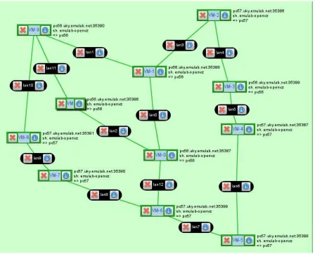
Figure 1. The single-aggregate experiment

side of the coin are experiments using multiple aggregates. For large network experiments, the number of nodes usually exceeds the number of aggregates available. We have to allocate multiple nodes within an aggregate. Thus, even in a multi-aggregate experiment, we may still have links within an aggregate. In either case, we need to have an idea about delays and bandwidth of both single-aggregate links and cross-aggregate links.

In this paper, we present our study on performance of GENI networks, with a focus on the tradeoff between single aggregate and multiple aggregates in the design of GENI experiments from the performance perspective. We will analyze how the links behave differently over a period of time. The data collected will shed some light on the design process for choosing where the nodes in the experiment should be located.

The rest of the paper is organized as follows. Section 2

presents related work and some background concepts. Section 3 describes the experiments we used to collect performance data. Section 4 presents the results about the latencies and bandwidth of the links within an aggregate and across aggregates. Section5concludes the paper.

2. Related Work

GENI has involved many universities and industry partners and grown significantly in recent years [5]. It consists of multiple control frameworks [6,7] and has resources mainly on university campuses in the United States and several sites in other countries. It developed many tools supporting experimenters, such as Flack [8, 9] of ProtoGENI [6]. It has been used both in education for teaching networking and distributed systems classes [10,11] and in research for exploring future Internet architectures and protocols [12].

Measurement for cross-layer communications has been studied in the GENI context [13]. It focused on embedding real-time measurement mechanism in the substrate, especially in the opitcal networks. Several early GENI projects investigated performance measurement [14–18] in the GENI environment. They have different focuses and generally emphasize on developing tools to enable users to collect performance data.

(3)

uky

clemson

gatech mu

wisc

nyu nw

uiuc utah

gpo

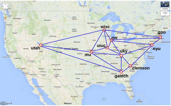
Figure 2. The multi-aggregate experiment

instrument resources based on the ORBIT control framework. It can filter and process measurement flows, and consume measurement flows. The other is the GENI Measurement and Instrumentation Infrastructure (GEMINI) project [20–22]. It is based on earlier INSTOOLS system [14] and perfSONAR system [23]. It started with supporting ProtoGENI, but can now support nodes from other control frameworks as well. All these GENI measurement systems emphasize on building tools to support users to collect measurement data after their experiments have been set up. In contrast, this paper focuses on examining behaviors of different kinds of links in GENI networks and help users in the design process of their experiments.

3. Experiments for Data Collection

To measure the performance of links within an aggregate, we design a 11-node topology as shown in Figure 1. In GENI, multiple virtual machines (VMs) can be allocated from a single raw physical machine/computer (PC). We want to measure both the links that connects two VMs from the same physical machine and the links that connects two VMs from two different physical machines. Theoretically, three VMs are enough because we can have two VMs from the same physical machine and the other one from a different physical machine. We can create both kinds of links with these three machines. However, if we create a topology with three VMs, most likely we will end up with three VMs from the same physical machine due to the allocation algorithm used in GENI aggregates. Even though we can bind a VM to a specific physical machine, the submission through the GENI Flack interface was not well supported at the time of our experiments. Our strategy is to specify a topology as shown in Figure1with enough number of nodes so that they have

to be allocated to different physical machines. We understand that we do not have to measure all the links. Rather we select four links as representatives.

We obtained the bandwidth and latency data for these four links using iperf[24] and pingover 10 days. One measurement (both bandwidth and latency) is taken for every hour, with 10ECHO_REQUESTs for each ping. We want to inspect whether there is a pattern depending on the time of a day or the day of the week. So we choose a duration that is long enough to cover more than a week. We understand that a longer duration will give us a more thorough picture of performance of the links. However, that is something we want to pursue in the future and is beyond the scope of this paper.

To measure the performance of links from different aggregates, we select 10 aggregates and set up a mesh topology as shown in Figure2. We request one VM from each aggregate and use GRE tunnels for the links connecting these VMs.

4. Performance Results

We collected both latency and bandwidth information from these two experiments. Links in these two experiments can be divided into three categories:

Category 1 (Same PC): the links connecting two VMs that are allocated from the same physical machine;

Category 2 (Same Aggregate): the links connecting two VMs that are allocated from two different physical machines located in the same aggregate; and

(4)

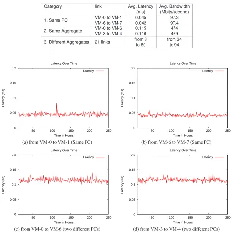
Table 1. Average latency and bandwidth

Category link Avg. Latency Avg. Bandwidth (ms) (Mbits/second)

1. Same PC VM-0 to VM-1 0.045 97.3

VM-6 to VM-7 0.042 97.4

2. Same Aggregate VM-0 to VM-6 0.115 474

VM-3 to VM-4 0.116 469

3. Different Aggregates 21 links from 3 from 34

to 60 to 94

0 0.05 0.1 0.15 0.2

50 100 150 200 250

Latency (ms)

Time in Hours Latency Over Time

Latency

0 0.05 0.1 0.15 0.2

50 100 150 200 250

Latency (ms)

Latency

(a) from VM-0 to VM-1 (Same PC) (b) from VM-6 to VM-7 (Same PC)

0 0.05 0.1 0.15 0.2

50 100 150 200 250

Latency (ms)

Latency

0 0.05 0.1 0.15 0.2

50 100 150 200 250

Latency (ms)

Latency

(c) from VM-0 to VM-6 (two different PCs) (d) from VM-3 to VM-4 (two different PCs)

Figure 3. Latency of the links connecting two VMs from the same aggregate

The first experiment covers the first two kinds of links (category 1 and category 2), while the second experiment covers the third kind of links (category 3). We first calculate the averages of latencies and bandwidths over the 10 day period for each link. The results are summarized in Table1.

The links in the Same PC category have similar performance. So we only choose two links (from VM-0 to VM-1, and from VM-6 to VM-7) as representatives. For the same reason, we only choose two links (from VM-0 to VM-6, and from VM-3 to VM-4) as representatives for the

Same Aggregate category. However, the performance of the links from the Different Aggregates category varies a lot. We summarize the results for the links in the second experiment in the table.

(5)

30 35 40 45 50 55

50 100 150 200 250

Latency (ms)

Latency

0 50 100 150 200 250 300 350 400 450

50 100 150 200 250

Latency (ms)

Latency

(a) from Kentucky to Missouri (b) from Utah to Gatech

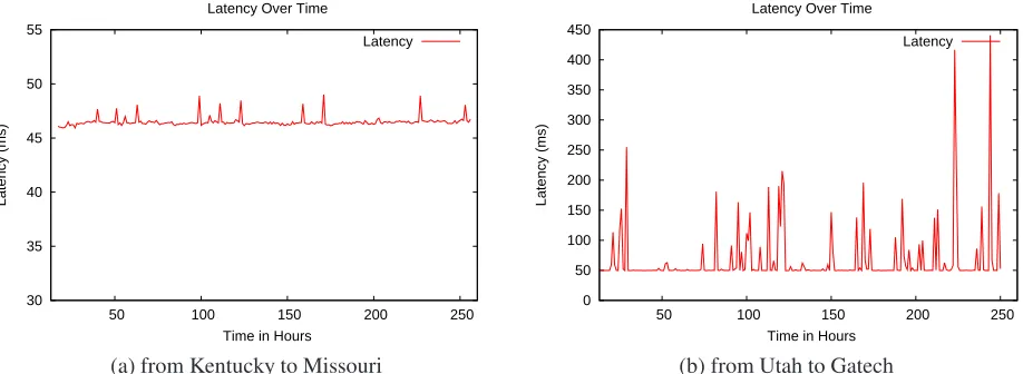
Figure 4. Latency of the links connecting two VMs from two different aggregates

0 0.2 0.4 0.6 0.8 1

0 0.01 0.02 0.03 0.04 0.05 0.06 0.07 0.08 0.09

Percent

Latency (ms) cdf of the latency

cdf of the latency

0 0.2 0.4 0.6 0.8 1

0 0.02 0.04 0.06 0.08 0.1 0.12 0.14 0.16

Percent

cdf of the latency

(a) Same Physical PC (b) Two Physical PCs

Figure 5. cdf of latency of links within an aggregate

lowest latency we got is the link connecting VMs from the Northwestern aggregate and the UIUC aggregate, measured at 3ms, which are 30 times as large as that of the links from the Same Aggregate category. We see a wide variety of latencies measured for different cross-aggregate links, ranging from 3ms to 60ms. When designing a GENI experiment, we may take the difference in latencies into consideration for reserving GENI resources.

While the average latencies give a general idea about the tradeoff between using nodes from a single aggregate versus from multiple aggregates, it is more interesting to observe how they change over time. Figure3(a) shows how the latency of the link from VM-0 to VM-1 in the first experiment change over the 10 day period. We can see that it always hovers around 0.045ms, with the highest at 0.084ms at one time and with the lowest at 0.034ms three times. It is relatively stable

and close to its average value. Figure3(b) shows that the link from VM-6 to VM-7 displays the similar pattern.

The latencies for the links connecting two VMs from two different PCs within an aggregate are larger than that of category 1 links as shown in Figure3(c) and (d). Also larger is the range these latencies change. However, we still see a very stable pattern in terms how they change over time.

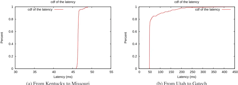
The latencies for category 3 links demonstrate a wider variety of patterns. For lack of space, we cannot present all of them in this paper. Instead, we choose two as representatives here to show how they can be quite different. Figure4(a) shows how the latency of the link from Kentucky to Missouri 1 _{change over time. The absolute range of the}

1_{We use abbreviations here to indicate the VMs from a certain aggregate.}

(6)

0 0.2 0.4 0.6 0.8 1

30 35 40 45 50 55

Percent

cdf of the latency

0 0.2 0.4 0.6 0.8 1

0 50 100 150 200 250 300 350 400 450

Percent

cdf of the latency

(a) From Kentucky to Missouri (b) From Utah to Gatech

Figure 6. cdf of latency of links cross aggregates

change is larger than those links from categories 1 and 2. However, the percentage of the change is not large. It is a totally different story for the link from Utah to Georgia Tech (Gatech) as shown in Figure4(b). Notice that the scales on y-axis in the figures are different. The range of the change in this case is almost 10 times as large as the average value. We can end up with a much more unpredictable behavior if we have VMs allocated from different aggregates.

To better understand the characteristics of the links from different categories, we plot the cumulative distribution functions (cdfs) of the latencies of these links in Figure 5

and Figure6. Since the two links from category 1 has similar behavior, we only include the cdf for the link from VM-0 to VM-1. We can see that most values are evenly distributed between 0.038ms and 0.05ms in Figure5(a). For the same reason, we only include the cdf for the link from VM-0 to VM-6 as the representative for category 2 links. We can see in Figure5(b) that most values are evenly distributed between 0.105ms and 0.125ms. In contrary, the cross-aggregate links have a different distribution. They have a lot of measured values close to a certain bottom value. In the case of the link from Kentucky to Missouri, more than 90% the latencies are between 46ms and 47ms, as shown in Figure6(a). The latency of the link from Utah to Gatech is between 49.5ms and 52.5ms in more than 75% of the cases, as presented in Figure6(b). These two links also have an obvious difference in that the cdf of the latency of the link from Utah to Gatech has a long tail because there are a significant number of values that are substantially larger than the average.

The latency of the links is only one factor to consider in designing GENI experiments. The other factor is the bandwidth of the links. From Table1, we can see that category 1 links have a measured bandwidth of 97.3 Mbps. It can

of Missouri GENI aggregate. We use this convention for naming other VMs, too.

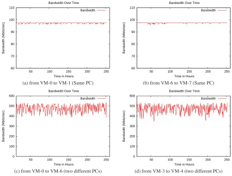
be higher because the two VMs these links attached to are located within the same physical machine. However, due to rate limit of the VMs, they are most likely capped at 100 Mbps. Figure7(a) and (b) shows how the bandwidth of these links change over time. Similar to the latency case, it stays close to the average level, appearing almost like a straight line.

Category 2 links achieve higher bandwidth, having average values at 474 Mbps and 469 Mbps. VMs in this case are connected with a gigabit switch. Because of the traffic from other experiments or load on the shared physical machines, the measured bandwidth is smaller than the maximal possible value. For the similar reason, we can see in Figure7(c) and (d) that it oscillates quite a lot over time, ranging from 347 Mbps to 533 Mbps. However, the bandwidth of category 2 links is still much large than that of both category 1 links and category 3 links.

We get a totally different picture for the links connecting two VMs from different aggregates. Depending on the links, we can get an average bandwidth as low as 34 Mbps and as high as 94 Mbps. They also change more wildly over time, as shown in Figure 8. This is because these links are cross-Internet links that will compete with traffic from other applications. Their behaviors are much more unpredictable than those links within a single aggregate. For the same link from Utah to Gatech, we can get a bandwidth measure as low as 8.5 Mbps and as high as 90.5 Mbps. If we want to observe how a protocol performs and reacts to the real world traffic, this may be the link we should include in the experiment.

(7)

60 70 80 90 100 110

50 100 150 200 250

Bandwidth (Mbits/sec)

Time in Hours Bandwidth Over Time

Bandwidth

60 70 80 90 100 110

50 100 150 200 250

Bandwidth

(a) from VM-0 to VM-1 (Same PC) (b) from VM-6 to VM-7 (Same PC)

0 100 200 300 400 500 600

50 100 150 200 250

Bandwidth

0 100 200 300 400 500 600

50 100 150 200 250

Bandwidth

(c) from VM-0 to VM-6 (two different PCs) (d) from VM-3 to VM-4 (two different PCs)

Figure 7. Bandwidth of the links connecting two VMs from the same Aggregate

0 10 20 30 40 50 60 70 80 90 100

50 100 150 200 250

Bandwidth

0 20 40 60 80 100

50 100 150 200 250

Bandwidth

(a) from Kentucky to Missouri (b) from Utah to Gatech

Figure 8. Bandwidth of the links connecting two VMs from two different aggregates

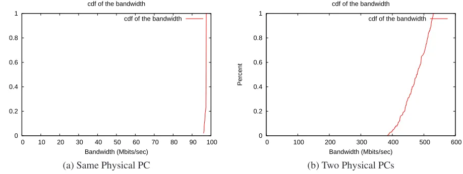
However, it is still relatively concentrated, as shown in Figure 9(b). The bandwidth for the links connecting VMs from different aggregates is distributed in a much wider range.

(8)

0 0.2 0.4 0.6 0.8 1

0 10 20 30 40 50 60 70 80 90 100

Percent

Bandwidth (Mbits/sec) cdf of the bandwidth

cdf of the bandwidth

0 0.2 0.4 0.6 0.8 1

0 100 200 300 400 500 600

Percent

(a) Same Physical PC (b) Two Physical PCs

Figure 9. cdf of bandwidth of links within an aggregate

0 0.2 0.4 0.6 0.8 1

0 20 40 60 80 100

Percent

0 0.2 0.4 0.6 0.8 1

0 20 40 60 80 100

Percent

(a) From Kentucky to Missouri (b) From Utah to Gatech

Figure 10. cdf of bandwidth of links cross aggregates

In summary, from the data we collected, we can see significant differences between single-aggregate links and cross-aggregate links in terms of latency and bandwidth. Not only the average values are significantly different, but their behaviors over time can be quite different as well. In general, the latencies of single-aggregate links are less than 0.2 ms while the latencies of cross-aggregate links are order of magnitude larger. For example, the latency between nodes from Utah to Georgia Tech can be somewher between 50ms to 400ms. The bandwidth of single-aggregate links ranges from 97Mbps to close to 500Mbps. The bandwidth of cross aggregate links is in the range from 34Mbps to 94mpbs. More importantly, the latency and bandwidth of single-aggregate links are more stable over time. In contrast, the latency and bandwidth of cross-aggregate links can go wildly and are more unpredictable. When designing a GENI experiment, we can make use of performance data to decide where the nodes in the experiment should be located to meet the requirement.

5. Conclusion

(9)

Acknowledgements. We would like to thank Dr. Jim Griffioen for his comments on our earlier work on this topic. We also want to thank Mr. Hussamuddin Nasir and other members of the GEMINI project team for their help during the design and implementation of this project.

This material is based upon work supported in part by the National Science Foundation under Grant No. CNS-0834243 and CNS-1346688 Subcontracts 1925 and 1928. Any opinions, findings, and conclusions or recommendations expressed in this material are those of the authors and do not necessarily reflect the views of BBN Technologies Corp, the GENI Project Office, or the National Science Foundation.

References

[1] THE GENI PROJECT OFFICE, GENI System Overview. Http://www.geni.net/docs/ GENISysOvrvw092908.pdf.

[2] GENI concepts. Http://groups.geni.net/geni/wiki/GENIConcepts. [3] GENI glossary. Http://groups.geni.net/geni/wiki/GENIGlossary. [4] GENI aggregates. Http://groups.geni.net/geni/wiki/GeniAggregate. [5] BERMAN, M., CHASE, J.S., LANDWEBER, L., NAKAO, A.,

OTT, M., RAYCHAUDHURI, D., RICCI, R. et al. (2014) GENI: a federated testbed for innovative network experiments.

Computer Networks61: 5–23. [6] ProtoGENI. Http://www.protogeni.net. [7] ORCA. Https://geni-orca.renci.org/trac/.

[8] (2012), The Flack GUI. Http://www.protogeni.net.

[9] DUERIG, J., RICCI, R., STOLLER, L., STRUM, M., WONG, G., CARPENTER, C., FEI, Z. et al. (2012) Getting started with GENI: A user tutorial. ACM SIGCOMM Computer Communication Review (CCR)42(1): 72–77.

[10] LAVERELL, W.D., FEI, Z. and GRIFFIOEN, J.N. (2008) Isn’t it time you had an emulab? InACM SIGCSE 2008 Technical Symposium on Computer Science Education. Portlan, Oregon. [11] GRIFFIOEN, J., FEI, Z., NASIR, H., WU, X., REED, J. and CARPENTER, C. (2013) GENI-enabled programming experiments for networking classes. InProc. of the Second GENI Research and Educational Experiment Workshop (GREE2013). Salt Lake City, Utah.

[12] New GENI shakedown experiments. http://groups.geni.net/ geni/wiki/GEC18Agenda/NewDocAndExpts.

[13] Embedding real-time substrate measurements for cross-layer communications. Http://groups.geni.net/geni/wiki/Embedded Real-Time Measurements.

[14] GRIFFIOEN, J., FEI, Z., NASIR, H., WU, X., REED, J. and CARPENTER, C. (2012) The design of an instrumentation system for federated and virtualized network testbeds. InProc. of the First IEEE Workshop on Algoirthms and Operating Procedures of Federated Virtualized Networks (FEDNET). Maui, Hawaii.

[15] GIMS: High-speed packet capture for GENI. Http://gims.wail.wisc.edu/docs/Tutorial.html.

[16] Leveraging and abstracting measurements with perfSONAR(LAMP). Http://groups.geni.net/geni/wiki/LAMP. [17] CALYAM, P. and SCHOPIS, P. (2012), OnTimeMeasure: Cen-tralized and distributed measurement orchestration software. Http://groups.geni.net/geni/wiki/OnTimeMeasure.

[18] FAHMY, S. and SHARMA, P. (2010), Scalable, extensible, and safe monitoring of GENI clusters. http://groups.geni.net/geni/attachment/wiki/ScalableMonitoring/ design.pdf.

[19] GIMI: Large-scale GENI instrumentation and measurement infrastructure. Http://groups.geni.net/geni/wiki/GIMI. [20] GEMINI: A GENI measurement and instrumentation

infras-tructure. Http://groups.geni.net/ geni/wiki/GEMINI.

[21] GRIFFIOEN, J., FEI, Z., NASIR, H., WU, X., REED, J. and CARPENTER, C. (2014) Measuring experiments in geni.

Computer Networks63: 17–32.

[22] FEI, Z., YI, P. and YANG, J. (2014) The tradeoff between single aggregate and mulitple aggregates in designing GENI experiments. InProc. of the 9th International Conference on Testbeds and Research Infrastructures for the Development of Networks & Communities (TridentCom). Guangzhou, China. [23] PerfSONAR. Http://www.perfsonar.net/.