Predicting ocean waves along the US east coast during energetic winter storms: sensitivity to whitecapping parameterizations

(1)

Ocean Sci., 15, 691–715, 2019

https://doi.org/10.5194/os-15-691-2019

Predicting ocean waves along the US east coast during energetic

winter storms: sensitivity to whitecapping parameterizations

Mohammad Nabi Allahdadi1, Ruoying He1, and Vincent S. Neary2

1_{North Carolina State University, Department of Marine, Earth, and Atmospheric Sciences, Raleigh, NC, USA} 2_{Sandia National Laboratories, P.O. Box 5800, Albuquerque, NM, USA}

Correspondence:Mohammad Nabi Allahdadi ([email protected]) Received: 3 October 2018 – Discussion started: 1 November 2018

Revised: 25 March 2019 – Accepted: 29 April 2019 – Published: 6 June 2019

Abstract. The performance of two methods for quantify-ing whitecappquantify-ing dissipation incorporated in the Simulat-ing Waves Nearshore (SWAN) wave model is evaluated for waves generated along and off the US east coast under en-ergetic winter storms with a predominantly westerly wind. Parameterizing the whitecapping effect can be done using the Komen-type schemes, which are based on mean spec-tral parameters, or the saturation-based (SB) approach of van der Westhuysen (2007), which is based on local wave pa-rameters and the saturation level concept of the wave spec-trum (we use “Komen” and “Westhuysen” to denote these two approaches). Observations of wave parameters and fre-quency spectra at four National Data Buoy Center (NDBC) buoys are used to evaluate simulation results. Model–data comparisons show that when using the default parameters in SWAN, both Komen and Westhuysen methods underes-timate wave height. Simulations of mean wave period using the Komen method agree with observations, but those using the Westhuysen method are substantially lower. Examination of source terms shows that the Westhuysen method underes-timates the total energy transferred into the wave action equa-tions, especially in the lower frequency bands that contain higher spectral energy. Several causes for this underestima-tion are identified. The primary reason is the difference be-tween the wave growth conditions along the east coast during winter storms and the conditions used for the original white-capping formula calibration. In addition, some deficiencies in simulation results are caused along the coast by the “slanting fetch” effect that adds low-frequency components to the 2-D wave spectra. These components cannot be simulated partly or entirely by available source terms (wind input, whitecap-ping, and quadruplet) in models and their interaction.

Fur-ther, the effect of boundary layer instability that is not con-sidered in the Komen and Westhuysen whitecapping wind input formulas may cause additional underestimation.

1 Introduction

Spectral wave models, including Simulating Waves Nearshore (SWAN) (SWAN, 2015), solve the equation for conservation of wave action density in the frequency– direction, spatial, and time domains. This equation considers the time variation of spectral energy over the specified geographic domain by considering the local rate of change and transport terms as well as source terms. The source term in the wave action density equation is the algebraic sum of several terms as follows:

(2)

692 M. N. Allahdadi et al.: Predicting ocean waves along the US east coast during energetic winter storms

The Komen-type methods for resolving whitecapping dis-sipation are some of the most popular approaches in coastal modeling applications and are based on the initial study by Hasselmann (1974), formulated by Komen et al. (1984), and modified by Janssen (1991). This approach represents dissi-pation of spectral energy as a function of mean spectral fre-quency and steepness. It is an appropriate approach for simu-lation of wave height as a result of generation and growth by local wind, and the default method for resolving whitecap-ping dissipation in SWAN and other popular spectral mod-els like WAM and Mike21-SW. To achieve higher simula-tion accuracies for wave height and wave period, calibra-tions of the model for the whitecapping parameter and the wave period parameter delta are necessary (Allahdadi et al., 2017; Siadatmousavi et al., 2012; Niroomandi et al., 2018; Allahdadi et al., 2004a). However, wave model applications for different regions (including open-ocean and shelf waters) show that Komen-type methods tend to underestimate both peak and mean wave periods (SWAN, 2015; van Vledder et al., 2016; Siadatmousavi et al., 2011). For the case of pure wind–wave growth, this problem is the result of underesti-mating the spectral energy at low frequencies. In the presence of low-frequency swells with lower spectral steepness, this method contributes to higher rates of swell energy dissipation and underprediction of wave period (van der Westhuysen et al., 2007). To address these shortcomings of the Komen-type models, van der Westhuysen et al. (2007) introduced an alter-native whitecapping method based on a modified approach by Alves and Banner et al. (2003) using the concept of lo-cal saturation of spectra instead of mean spectral parameters. This method, known as the saturation-based (SB) approach, was successfully applied to several cases of sea–swell com-binations and outperformed the Komen-type approaches (van der Westhuysen et al., 2007, hereafter W007; Mulligan et al., 2008). W007 evaluated the above two types of white-capping formula by comparing SWAN modeling results and field observations for coastal and inland waters including the shelf waters of North Carolina and the shallow Lake Ijssel the Netherlands. Mulligan et al. (2008) employed SWAN to study the evolution of waves in the semi-enclosed Lunenburg Bay in Nova Scotia under the effect of local waves gener-ated by an extratropical storm and swells from the northwest-ern Atlantic. However, these applications were mostly imple-mented for settings with limited fetch lengths, such as lakes, bays, and small coastal areas (with limited fetch lengths on the order of 100 km or smaller), and shorter study periods, so that time variations of the wind field were not considered.

During the recent years, several combinations of newer wind input/whitecapping formulations were developed and incorporated in the WAVEWATCHIII (WWWIII) model. These models, including ST2, ST4, and ST6, were devel-oped to be more consistent with physics of wind–wave/swell dissipation rather than only the mathematical balance that was the base for the previous formulations like Komen-type and Westhuysen (Babanin and van der Westhuysen, 2008;

Tolman, 2014). The most recent formulation (ST6) is ba-sically an observation-based scheme that also includes the effect of negative wind input and wave–turbulence interac-tion. Although the ST6 physics package has been included in SWAN 41.20, there is limited experience with this physics package in coastal waters. Furthermore, the range of applica-bility of W007 for larger fetches with inhomogeneous wind fields is poorly known regardless of the fact that this formu-lation and the Komen-type approaches are still extensively being used for wave modeling of different regions all over the world. Therefore, it is imperative to examine these ap-plication ranges for different regions. Otherwise, extensive efforts may be required for model sensitivity analysis and calibration (Chaichitehrani, 2018; Allahdadi et al., 2019).

(3)

M. N. Allahdadi et al.: Predicting ocean waves along the US east coast during energetic winter storms 693

be considered by atmospheric models with hourly to several hourly outputs (Abdallah and Cavaleri, 2002). To be consis-tent with the practical modeling efforts and real applications, we did not correct the wind field for gustiness. Therefore, in our simulation, we used a wind field with 1 h temporal res-olution that cannot include such short-term variations (see Sect. 4 for details).

The present study was motivated by a recent 31-year simu-lation that authors implemented for the US east coast to char-acterize wave energy resources (Allahdadi et al., 2019). We used SWAN for this modeling since due to complex coastal geometry we could benefit from the flexible mesh option made available by SWAN. The only whitecapping formula-tions that are available by SWAN-ADCIRC (we had to use this coupled version to implement the domain decompos-ing needed for the high-performance computation over more than 4 300 000 computational grid points) are Komen-type and Westhuysen approaches. During the study, we had to per-form extensive sensitivity and calibration to select the most appropriate whitecapping approach amongst the ones avail-able in SWAN and a part of these efforts is reported here. The main research questions that will be answered through the present study are what the appropriate ranges are of appli-cations for Komen and Westhuysen whitecapping formula-tions (see Sect. 2 for detailed formulaformula-tions) for the geograph-ical extent of the US east coast and under the outbreak of the winter storms, and what the effects are of different wind conditions and other factors like coastal geometry and insta-bilities in the air–sea boundary layer on evolution of waves under these circumstances. The relatively large fetches and non-stationary large wind fields that are common for the real cases of wave generation and propagation over extensive re-gions are examples of the cases that need further attention.

It should be noted that the main goal of the present study is examining the performance of these whitecapping formulas within a real simulation framework, not a detailed examina-tion of the theoretical basis. Through this study, the perfor-mance of these two whitecapping formulations is evaluated against in situ observations using simulations for the US east coast coastal ocean. Wind and wave fields over this area fol-low a seasonal pattern with most energetic wind–wave events in late fall and early winter (Allahdadi et al., 2019). During the summer, the effect of swells with longer periods is more pronounced over the study area, an additional component that may cause differences in the performance of Komen-type and SB whitecapping approaches. Hence, a separate model performance evaluation for each season is warranted. The present paper is dedicated to implementing this evaluation during January 2009. The persistent offshore-ward wind field during this month (Allahdadi et al., 2019), along with large fetch lengths over the modeling region, provides an appro-priate condition to study different features of wind field and waves including fetch-limited and fully developed sea states.

2 Source term quantification for whitecapping and wind input

The default approach for quantifying whitecapping dissipa-tion in SWAN is the pulse-based, quasi-linear model of Has-selmann (1974) that was formulated by Komen et al. (1984):

Sds,w(σ, θ )= (2)

−Cds

(1−δ)+δk ek e S e SPM !p eσ k ek E (σ, θ )

eS=ek p

Etot, (3)

whereCdsis the whitecapping coefficient andδis a param-eter for partially adjusting the wave period that varies be-tween 0 and 1 with the default of 1 in SWAN. It may also affect the wave height and one may need to change it in agreement withCds. Rogers et al. (2003) reported that by changingδ from 0 to 1 the accuracy for prediction of wave energy corresponding to low-frequency increases. Parame-terp is a constant,k is wave number with the average of ek,σ is the angular wave frequency with the average of_eσ, Etot is the total energy of the wave spectrum,eS is the mean spectral steepness, andeSPM=(3.02×10−3)1/2is the mean spectral steepness due to the Pierson–Moskowitz spectrum (SWAN, 2015). Average angular frequency and average wave number are calculated by integration over the frequency– directional spectrum as Etot/R Rσ−1E (σ, θ ) dσ dθ and h

Etot/R Rk−

1

2_{E (σ, θ ) dσ dθ}

i2

, respectively. The strong de-pendency of the formulation on the mean spectral parameters is maintained throughek,_eσ, andeS. Two sets of values forCds andpwere found by Komen et al. (1984) and Janssen (1992) by balancing the energy equation through fetch growth tests. The Komen-type whitecapping method is conjugated with a wind input term that includes both linear and exponential growth terms (SWAN, 2015):

Sin(σ, θ )=A+BE(σ θ ). (4)

In SWAN, the linear term (A) is estimated by a formulation of Cavaleri and Rizzoli (1981). The exponential growth term (the term including the coefficient B) is a function of the spectral energy and accounts for the main energy input by the wind. The coefficientBfor Komen et al. (1984) is calculated based on the wave age inverseu∗

c and angular frequency:

B=max

0,0.25ρa ρw

(28u∗

c cos(θ−θw)−1)

σ, (5)

whereu∗is the wind shear velocity,cis wave phase speed, ρaandρw are air and water densities, respectively,θ is the direction of spectral component for which wind input is cal-culated, andθwis the wind direction.

(4)

methods due to the dependency of this process on the mean spectral parameters. The attempts mostly focused on remov-ing the dependency on the mean spectral steepness and wave number. Alves and Banner (2003) presented a new form that related the wave groups to the whitecapping dissipation. This form was adopted and modified by W007 and was incorpo-rated into SWAN as the SB model for whitecapping. This approach assumes that whitecapping dissipation affects wave groups when reaching a specific threshold:

Sds,break(σ, θ )= (6)

−Cds

B(k) Br

p/2

[tanh(kd)]

2−p₀

4 p_{gkE(σ θ )}

B (k)=

2π

Z

0

cgk3E (σ, θ ) dθ (7)

p=p0

2 + p0 2 tanh " 10 s B(k) Br −1 !# . (8)

In the above equations,p0is a function of the wave age in-verse u∗

c, d is water depth, g is acceleration due to

grav-ity, and cg is the wave group velocity. B(k) is defined as the azimuthal-integrated spectral saturation andBr =1.75×

10−3is the threshold saturation level. IfB (k) > Br, waves

break due to whitecapping. The dependency of the dissipa-tion equadissipa-tion on group velocity and the associated satura-tion level for each wave group leads to separate estimasatura-tion of the whitecapping dissipation for seas and swells and re-duces their unrealistic interaction that significantly affects the whitecapping dissipation over different parts of the spec-trum. In the version of SB whitecapping that is incorporated in SWAN, an additional term has been used for inclusion of dissipation caused by turbulence and interaction between long and short waves. Thus, the final whitecapping dissipa-tion term is a weighted sum of the dissipadissipa-tion due to breaking and non-breaking waves:

Sds,w(σ θ )=fbr(σ ) Sds,break

+ d1−fbr(σ )eSds,non−break. (9)

In the above equation,fbr(σ )is a function ofB (k)andBr

that provides a smooth transition between the breaking and non-breaking components of the dissipation.

Finally, a consistent wind input expression that consid-ers the exponential wave growth by wind, suggested by Yan (1987), is used in conjunction with the SB whitecapping approach. This expression is obtained based on the labora-tory and field measurements that show quadratic growth for

u∗

c >0.1 (e.g., Plant, 1982; Peirson and Belcher, 2005) and

linear growth for u∗

c <0.1 (Snyder et al., 1981; Hasselmann

and Bösenberg, 1991):

B=D _u∗

cph 2

cos(θ−θw)+E _u∗

cph

cos(θ−θw)

+Fcos(θ−θw)+H, (10)

whereD,E,F, andH are coefficients of the fit (W007).

3 Modeling domain and field data

The modeling area includes the US east coast from the Gulf of Maine to southern Florida and the offshore areas west of 61.0◦W (Fig. 1). This area is characterized by seasonal vari-ations of winds (Allahdadi et al., 2019). For example, dur-ing January 2009, the average wind direction along and off the US east coast was northwesterly to westerly with aver-age wind speed of 6.5 m s−1, while for July 2009 average wind direction was southwesterly with average wind speed of 3.5 m s−1. During the late fall and the entire winter, the study area, especially the northern part, is significantly affected by extratropical storms with strong westerly winds that gener-ate coastal and offshore waves with the general direction of west to east (Allahdadi et al., 2019). In the present study, the evolution of waves is investigated during January 2009.

The performance of the two whitecapping methods was evaluated at four National Data Buoy Center (NDBC) buoys, including two in the north part of the modeling area (44017 nearshore and 44011 offshore) and two in the south (41004 nearshore and 41048 offshore) (Fig. 1 and Table 1). Wave height, peak wave period, mean wave period, wind speed, frequency spectra, and other met-ocean parameters were collected at these buoys.

(5)

Figure 1.Modeling area and locations of National Data Buoy Center (NDBC) buoys used for evaluation of whitecapping models.

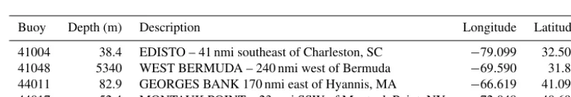
Table 1.Information on NDBC stations used for evaluation of model results.

Buoy Depth (m) Description Longitude Latitude

41004 38.4 EDISTO – 41 nmi southeast of Charleston, SC −79.099 32.501

41048 5340 WEST BERMUDA – 240 nmi west of Bermuda −69.590 31.86

44011 82.9 GEORGES BANK 170 nmi east of Hyannis, MA −66.619 41.098

44017 52.4 MONTAUK POINT – 23 nmi SSW of Montauk Point, NY −72.048 40.694

4 Model setup

A high-resolution unstructured SWAN model (coupled with ADCIRC for implementing the domain decomposition in the parallel mode) with a coastal resolution of 200 m was devel-oped and applied in this study. Details of the model setup are given in Allahdadi et al. (2019). Model bathymetry was prepared using two data sources, including a high-resolution database from NOAA’s Coastal Relief Model with a spa-tial resolution of 3 arcsec (∼90 m) for the coastal areas and NOAA’s ETOPO1 Global Relief Model with a spatial reso-lution of 1 min (∼1700 m) for deep and offshore areas. The model was forced by wind fields from the NCEP Climate Forecast System Reanalysis (CFSR) with a spatial resolution of 0.312◦_{(almost 32 km for the east coast region) and} tem-poral resolution of 1 h. Evaluation of CFSR wind fields at different buoys showed the good accuracy of these data for the east coast region (Fig. 4). For the four stations for which the CFSR wind field were evaluated in Fig. 4, the correlation coefficient varies between 0.88 and 0.92, and the bias is as low as −0.06 m s−1, which shows the general underestima-tion trend of the simulated wind speed by the CFSR. This underestimation is especially pronounced for higher wind

(6)

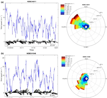
Figure 2.Time series of measured wind speed (lines) and vectors (arrows) and the associated wind roses at NDBC buoys 44011(a)and 41048(b).

boundaries, the model was forced using the wave parame-ters obtained from a global WWWIII model with a spatial resolution of 0.5◦ and temporal resolution of 3 h. Follow-ing Whalen and Ochi (1978), Ochi (1998), and Allahdadi et al. (2004b), a Joint North Sea Wave Project (JONSWAP) frequency spectrum with the average enhanced parameter of γ =3.3 was chosen for converting parametric wave data to 2-D spectra along the boundary. Due to the dominant west-to-east wind over the modeling area during the simulation pe-riod, it is less likely for boundary waves to propagate toward the modeling area. Nevertheless, realistic boundary data were used in this study. The number of spectral directions and fquencies for discretization of 2-D spectra were 24 and 28, re-spectively. Simulation was done using a minimum frequency of 0.04 Hz, maximum frequency of 1.00 Hz, a computational time step of 10 min, and three computational iterations per time step (Allahdadi et al., 2019). Source terms for white-capping dissipation and their associated wind input

formu-lation were examined based on the two types of whitecap-ping dissipation approaches discussed in Sect. 2. For the rest of source terms, including quadruplets, triads, depth-induced wave breaking, and bottom dissipation, the default methods in SWAN were used.

5 Results

(7)

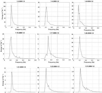
Figure 3.Examples of single-peaked frequency spectra measured at NDBC 44011 in January 2009. The title for each panel shows the date and time of measurement with the format month–day–year–hour: minute.

simulated mean wave period that is used for model evalua-tion as well as the mean wave direcevalua-tion that is later used for representing the wave vectors are presented below:

Tm02=2π( RR

ω2E(ω, θ )dω dθ R R

E (ω, θ ) dω dθ )

−1/2 ₍₁₁₎

Dir=arctan

R_sin_{θ E (ω, θ ) dω dθ} R

cosθ E (ω, θ ) dω dθ

. (12)

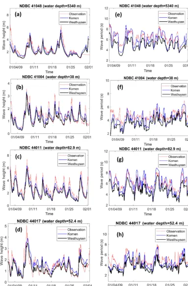
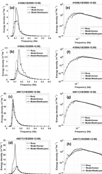
In the above equations, Tm02 is the mean wave period, ω is the radian frequency of a specific wave energy compo-nent, θ is the direction of wave energy component,E(ωθ) is the corresponding wave energy for this spectral compo-nent, and Dir is mean wave direction. Comparisons with field data show that both whitecapping approaches under-estimate wave height and wave period (less pronounced for Komen) at all stations. For all stations, Westhuysen simu-lated smaller wave heights compared to both observations and Komen (Fig. 6a to d). While at all four stations West-huysen significantly underestimated the wave period (Fig. 6e

to h), wave periods from Komen differed from observations at some stations. Comparison results for wave height and pe-riod as obtained from measurements and simulation scenar-ios for t1 and t2 show similar patterns (Table 2). It should be noted that SWAN uses a prognostic high-frequency tail for integration over a full frequency range that can increase the integration range to 10 Hz (SWAN, 2015). Since buoys integrate parameters over a narrow spectral range (in the case of NDBC buoys of the present study the range is 0.02– 0.485 Hz), some additional discrepancies may be introduced to the comparisons between model and buoy parameters. Akpinar et al. (2012) showed that these discrepancies are negligible for wave height and could only be important for lower values of wave periodTm02(approximately lower than 3 s). Since the measured wave periods during our simulations at all four buoys are larger than 3 s for most times (Fig. 6e– h), we can safely neglect this discrepancy for the wave period comparison.

(8)

Figure 4.Evaluation of the CFSR wind field versus measured wind by NDBC buoys at four stations shown in Fig. 1.

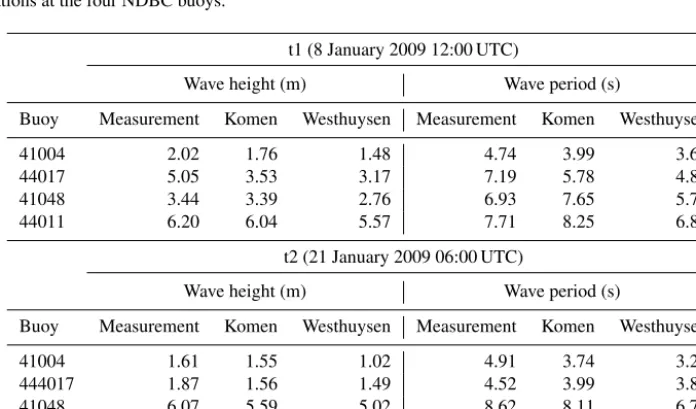
Table 2. Simulated wave heights and mean periods using Komen and Westhuysen whitecapping methods at reference times t1 and t2 compared to observations at the four NDBC buoys.

t1 (8 January 2009 12:00 UTC)

Wave height (m) Wave period (s)

Buoy Measurement Komen Westhuysen Measurement Komen Westhuysen

41004 2.02 1.76 1.48 4.74 3.99 3.61

44017 5.05 3.53 3.17 7.19 5.78 4.89

41048 3.44 3.39 2.76 6.93 7.65 5.74

44011 6.20 6.04 5.57 7.71 8.25 6.83

t2 (21 January 2009 06:00 UTC)

Wave height (m) Wave period (s)

Buoy Measurement Komen Westhuysen Measurement Komen Westhuysen

41004 1.61 1.55 1.02 4.91 3.74 3.23

444017 1.87 1.56 1.49 4.52 3.99 3.84

41048 6.07 5.59 5.02 8.62 8.11 6.70

(9)

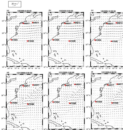
Figure 5.The 3-hourly snapshots of CFSR wind fields over the modeling area ending at times t1 (8 January 2009 12:00 UTC,a–c) and t2 (21 January 2009 06:00 UTC,d–f).

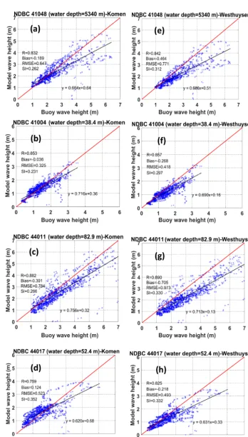
scatter plots (Figs. 7 and 8). Comparisons are quantified us-ing standard metrics for model performance includus-ing corre-lation coefficient (R), bias, root mean square error (RMSE), and scatter index (SI) (Tehrani et al., 2013). Statistics for wave height show that while the correlation coefficient of the matchup comparison is slightly larger for the Westhuy-sen, at all four buoys, the average errors of the simulated wave heights (bias) and the average distance from the ideal agreement line (RMSE) are significantly smaller for Komen (Fig. 7). The only exception is the RMSE for buoy 44017, for which the corresponding value of RMSE from Komen is just slightly larger than that of Westhuysen (0.52 for Komen and 0.49 for Westhuysen; see Fig. 7c). Scatter indices, which show the scattering of simulated values around the ideal matchup line, are smaller at buoys 41004, 41048, and 44011

for simulated wave heights by Komen. Again, the exception is buoy 44017. This different behavior is due to the com-plex coastal geography upwind of the station that causes the slanting fetch effect when the prevailing wind is from land toward offshore (Ardhuin et al., 2007). This effect will be further examined in Sect. 6. For simulated mean wave pe-riods, the correlation coefficients between the two scenarios are very similar at all buoys (Fig. 8). However, the remaining performance statistics significantly favor the Komen white-capping predictions. For all buoys, Westhuysen substantially underestimates the mean wave period with the RMSE values between 1.1 and 1.6 s, while for the Komen method, RMSEs range between 0.85 and 1.05 s.

(10)

(11)

(12)

(13)

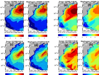
Figure 9.Simulated wave height (Hm0) and direction over the modeling area using Komen and Westhuysen whitecapping formulas for times t1(a, b)and t2(c, d)and simulation results for mean wave periods (T_m02) for times t1(e, f)and t2(g, h).

also investigated by examining snapshots of results over the modeling area (Fig. 9 for the results at time t1). It is worth noting that times t1 and t2 were not selected arbitrarily. They were selected so that at offshore buoys 44011 and 41048 al-most spatially uniform wind fields with sufficient durations occurred between land and the location of buoys so that the fetch-limited sea states are achieved at these buoys (Coastal Engineering Manual, 2006). This specific sea states will later be used for further discussions on the behavior of the white-capping formula. At time t1, significant differences are ob-served between wave heights from the twin simulations, es-pecially within the extensive region in the north that was af-fected by the intense storm winds (Fig. 9a and b). Similarly, at time t2 (Fig. 9c and d), significant differences result for the extensive areas offshore of North Carolina to New Jer-sey that are close to the instantaneous center of the storm. At both t1 and t2, substantial differences are observed between simulated wave periods (Fig. 9e to h). At t1 (Fig. 9e and f), wave periods off the New York coast are significantly under-estimated by Westhuysen compared to Komen (period of 7 s for Westhuysen and 9 s for Komen), a pattern that is also ob-served for time t2 (Fig. 9g and f) for all offshore areas off the Florida to Massachusetts coast.

To examine the performance of each whitecapping ap-proach in the simulation of wave energy distribution,

fre-quency spectra from two experiments were compared with measured spectra at each buoy and for t1 (Fig. 10) and t2. Hourly frequency spectra at the buoys are available from ob-servations for the frequency band of 0.02–0.485 Hz. How-ever, spectral energy corresponding to frequencies smaller than 0.06 Hz was zero. To minimize the effect of measure-ment noises at t1 and t2, measured spectra were averaged within a 3 h time window (W007). At each location, fre-quency spectra were also presented in semilogarithmic scale on the energy axis to more clearly show the differences.

(14)

(15)

that of measurements at time t1 is due to the persistent winds with almost constant speed and direction from the coast to-ward the station at this time and several hours before it (at least 6 h; Fig. 5). This wind condition can produce the fetch-limited wave growth with the well-developed single-peaked spectrum (Hasselmann et al., 1973) that can likely be sim-ulated by different whitecapping formulations because they are evaluated and calibrated mainly based on the measured fetch-limited growth curves (W007, Ardhuin et al. 2007). Discrepancies at the two coastal stations are caused by the effect of land roughness on the CFSR wind over the coastal areas (Allahdadi et al., 2019), non-persistence of wind field over these areas, and effect of slanting fetch (Ardhuin et al., 2007). The fetch-limited wave growth at 44011 is of particu-lar interest due to available field observations and modeling studies (for instance, Kahma and Calkoen, 1992). As men-tioned above, at this station at t1, the Komen approach shows almost identical values for the peak of energy and peak fre-quency to the measurements, while Westhuysen underesti-mates the peak of energy and overestiunderesti-mates the peak fre-quency. These results are in contradiction to the simulation result of W007 for a wave evolution test off the coast of North Carolina, USA. Their result showed that in the absence of offshore swells, the SB approach (Westhuysen) simulated higher levels of spectral energy corresponding to the peak frequency than those of Komen. Also, the simulated peak frequency from the SB model was more consistent with mea-surements. These different behaviors could be due to differ-ent growth conditions and wave age stages discussed in the next section.

Similar patterns to time t1 for comparison of simulated frequency spectra based on twin simulations and measure-ments are observed at time t2 (not shown). Because at this time the most persistent winds occur in the middle part of the modeling area, NDBC 41048 shows the best consistency for spectral energy and peak frequency.

6 Discussion

6.1 Examining source terms

A part of discrepancies in the simulation results from both whitecapping formulations is caused by inaccuracies in the wind field (see Fig. 4) mainly due to general underestima-tion of the wind speed by the CFSR wind that results in un-derestimations in the simulated wave heights and wave pe-riods. A calibrated model for the same study region as in this paper implemented by Allahdadi et al. (2019) resulted in the average bias of 0.11 m for significant wave height at different buoys. For the present study, the average bias val-ues for wave height are 0.19 and 0.33 m for simulations with Komen and Westhuysen whitecapping, respectively. If we conservatively assume that the whole bias in the calibrated model is attributed to the wind, more than half of the bias

in simulation with Komen and one-third of the bias for sim-ulation with Westhuysen whitecapping in the present study would be related to the wind. However, still significant differ-ences are observed between simulation results from Komen and Westhuysen considering the fact that both used the same wind field. Simulation results presented in the previous sec-tion clearly show that, compared to the in situ observasec-tions, the Komen whitecapping approach results in higher accuracy for both wave height and period. Over the modeling area, especially close to the instantaneous center of the storms at times t1 and t2, simulated wave heights and periods from Komen are larger than those of Westhuysen (Fig. 9).

Spatial and temporal variations of source terms (integrated source term magnitudes) for wind input (Swind), whitecap-ping dissipation (Swc), and quadruplet (Snl4) were obtained from SWAN simulations and diagnosed at these two times for both simulations to illustrate the contribution of source terms in the simulation results (Fig. 11). For each modeling simulation, the three essential source terms are of the same order of magnitude and show similar values. This is consis-tent with van Vledder et al. (2016). The quantified source terms by Westhuysen are significantly larger than those of Komen. For example, off the coast from New York Harbor to the Gulf of Maine, the estimatedSwindby Komen varies be-tween 1.5 and 2×10−4m2s−1, whereas the simulated wind input source term by the Westhuysen approach is at least twice as large as Komen’s. This is because the wind input term is a direct function of u∗

c in both formulations, but the

wind input formulation for Komen (Eq. 5) is a linear function of this parameter and is mostly appropriate for weaker wind speeds up to 12 m s−1(W007). Conversely, the wind input as-sociated with Westhuysen whitecapping (Yan, 1987; Eq. 10) is appropriate for both weak and strong wind forcing and in-cludes generation of wind energy as a function of both u∗

c

and(u∗

c)

2_{. The wind input formulation for each whitecapping} approach has been selected to be consistent with the scaling of the whitecapping to appropriately simulate the observed shape of the evaluated frequency spectra (W007) and keeping the total balance appropriate. Particularly for the spectral tail with frequencies 1.5 times higher than the peak frequency, Resio and Perrie (1991) reported that the dominant shape of the spectrum is a form which is a function off−4(f is wave frequency) for both weakly and strongly forced waves. This shape results from the stabilizing effect of the quadruplet in-teractions. Hence, spatial variations of whitecapping dissipa-tion for each approach are of the same order of magnitude as their wind input counterpart. Similar to the wind input, the simulated whitecapping using Westhuysen shows higher val-ues than those simulated by Komen. Compared to wind input and whitecapping, estimated quadruplet source terms as a re-sult of using Komen and Westhuysen are closer in value.

(16)

quadru-706 M. N. Allahdadi et al.: Predicting ocean waves along the US east coast during energetic winter storms

Figure 11.Spatial variations of source terms (wind input, whitecapping dissipation, and quadruplet in m2s−1) integrated in the spectral domain over the modeling area at time t1, for(a–c)Komen and(d–f)Westhuysen.

plet, their algebraic sums (sum of the first three right-hand terms in Eq. 1) are also compared in the frequency domain. The oscillatory variations of the quadruplet term with fre-quency, especially the ones for Westhuysen simulation could be due to oscillations of the whitecapping term between fre-quencies of 0.1 and 0.35 Hz (see Fig. 12b). This pattern has also been simulated by Mulligan et al. (2008). Like the in-tegrated values of these source terms over the modeling area (Fig. 11), variations of source terms versus frequency show larger values of wind input and stronger whitecapping dissi-pation by the Westhuysen approach (Fig. 12a and b). The algebraic sum of the source terms is the ultimate energy amount that is produced at each time step due to source term interactions and is subjected to spatial and temporal vari-ations based on the equation of wave action conservation. Hence, variations of this term in the frequency domain can be consistent with the shape of the energy–frequency spectra of Fig. 10. Komen simulated a larger sum of source terms at

(17)

Figure 12.Variations of simulated source term components with frequency at buoy 44011 for t1:(a)wind input,(b)whitecapping dissipa-tion,(c)quadruplet, and(d)algebraic sum of these terms.

6.2 Effect of wind field and growth conditions

In this section, the deficiencies associated with the Komen and Westhuysen whitecapping methods are investigated based on wave growth conditions during the simulation pe-riod. The performance of these two approaches for quanti-fying whitecapping dissipation and their wind input coun-terparts highly depends on the spatial and temporal varia-tions of the wind field and the spatial scale of the mod-eling area, which both affect wave growth. Hence, devel-oped approaches for wind input and whitecapping are pri-marily calibrated and verified using observed growth curves. These growth curves are represented in the form of non-dimensional energy and non-non-dimensional frequency both versus non-dimensional fetch X∗=gX/u2∗, whereX is the fetch length. W007 verified both the SB (Westhuysen) and Komen (using the default SWAN parameters like the present study) whitecapping approaches versus the growth curves of Kahma and Calkoen (1992) (for fetch-limited growth) and Pierson and Moskowitz (1964) (for the fully developed sea state) and determined the default calibration parame-ters for the SB model. The comparisons showed that, us-ing the default parameters for whitecappus-ing, both approaches performed well during the fetch-limited growth when the value of the non-dimensional fetches is<107, although for X∗ values between 104 and 105, the Westhuysen approach

(18)

under-708 M. N. Allahdadi et al.: Predicting ocean waves along the US east coast during energetic winter storms

Figure 13.Variations of the normalized whitecapping dissipation (Swcap) from Komen and Westhuysen simulation scenarios with the inverse wave age u∗

c at(a,c)NDBC 44011 and(b,d)NDBC 44017. Gray boxes indicate the fully developed zone (0.033< u∗

c <0.05). The dashed

line separates zones for linear and quadratic growth based on Yan (198y) as indicated byu∗

c =0.1.

estimation in both wave height and wave period is expected. However, in this area of the growth curve, Komen gener-ates higher levels of energy, i.e., higher wave heights result (Fig. 6). For the other offshore station (41048), even larger values forX∗on the order of 108–109are obtained that cor-respond to larger underestimations that are also evidenced in Fig. 6. At t2 and 6–10 h before that, the wind at buoy 41011 was consistently from the northeast with average speed of 7 m s−1, corresponding to a strong fully developed sea state with X∗≈108. At this time, the wave height was signifi-cantly underestimated by both whitecapping approaches, es-pecially by Westhuysen (Table 2). At coastal stations, how-ever, due to the generally short fetch lengths during the win-ter storm outbreak, fully developed sea states were less likely. For instance, at both t1 and t2, the persistent wind at buoy 41017 corresponded toX∗=5×106and 4.3×106, respec-tively, indicating fetch-limited growth.

Wind input and whitecapping source terms for both Komen and Westhuysen are direct or indirect functions of the wave age inverse u∗

c (Eqs. 5, 8, and 10). Multiple

stud-ies reported that with increasing wave age (decreasing the wave age inverse), dissipation due to whitecapping decreases (W007; Longuet-Higgins and Smith, 1983; Katsaros and Ataktürk, 1992). Wave age inverse is also an appropriate manifestation of the sea state and an indicator of whether

the sea state is in the forcing phase or fully developed. Volov (1970) and Oost (1998) suggested and Drennan and Graber (2003) later confirmed that a developing sea cor-responds to u∗

c >0.05, while 0.033< u∗

c <0.05 indicates a

fully developed sea state. For offshore buoy 44011 and nearshore buoy 44017, variations of simulated hourly white-capping dissipation with the inverse wave age for two exper-iments are plotted in Fig. 13. Since the scaling of the white-capping formula in Komen and Westhuysen differ (Fig. 11), simulated whitecapping values on the vertical axes are nor-malized based on the maximum value in each case. At both stations and for both whitecapping methods, whitecapping dissipation increases with increasing inverse wave age, al-though the nearshore station has more scattering due to the fetch length variations caused by the coastline irregularities. At the offshore station 41011 (Fig. 13a and c), significant numbers of events are included in the fully developed zone. The density of the simulated incidents in this zone decreased for the coastal station due to smaller fetch lengths. Based on the criteria specified by Volov (1970) and Oost (1998) and the calculated values ofu∗

c for simulation outputs, frequency

(19)

Figure 14.Frequency of occurrence for “developing” and “fully developed” sea states (based on Volov, 1970, and Oost, 1998) at stations 44011 and 44017 from buoy data and simulations using Komen and Westhuysen whitecapping formula.

of these two NDBC stations were used to calculate the FO values for two sea states. Comparisons showed that at both locations the FO for developing sea state was significantly overestimated by both models, although Komen simulated more consistent values of FO with those of buoys. This de-veloping sea state during which wind energy is actively trans-ferred from wind to water can be corresponding to either fetch-limited or duration-limited wave growths. For the fully developed sea states, Komen and Westhuysen compare dif-ferently at the costal and offshore buoys. At offshore buoy 44011, Komen simulated almost the same FO as the buoy observations, while Westhuysen underestimated the FO by 7 %. Both models underestimated the FO for the fully de-veloped sea state at the coastal station, but again Komen’s performance is slightly better. These results show that for the two major sea states resulted from generation and prop-agation of wind–waves, especially for the developing state, Komen and Westhuysen whitecapping formulas, may present substantially different features with those of measurements.

The above discussion shows that, for the east coast, a significant part of the deficiencies at offshore buoys (and to some extent at nearshore buoys) is caused by the spec-tral energy underestimation/peak frequency underestimation by these approaches during fully developed sea states. This could be fixed by revisiting the models’ calibration process and selecting smaller amounts for the default whitecapping parameter (Cdis) corresponding to the large values of the non-dimensional fetches. The default value for Komen white-capping as presented by Komen et al. (1984) is 2.3×10−5, while for the Westhuysen approach, W007 suggestedCds= 5×10−5 based on comparisons with field measurements. However, the modified whitecapping parameter for the fully developed condition may cause inconsistencies in the fetch-limited zone of the growth curve regarding the fact that the simulated non-dimensional energies and peak frequencies al-ready match the measurements. Hence, it is suggested that in future modifications, if possible, fully developed and fetch-limited conditions are treated independently, so that models could be able to calculate the whitecapping parameters based on the instantaneous non-dimensional fetches. Furthermore,

within an extensive modeling area with a high spatially and temporally variable wind field, an ideal fetch-limited con-dition is less likely to occur, at least for offshore areas, for the east coast during winter storms. The large fetch lengths for these areas need several hours of persistent winds with small variations in speed and direction to develop a fetch-limited condition. If variations of wind speed and direction occur often, the conditions for reaching a fetch-limited or fully developed sea state are violated (Coastal Engineering Manual, 2006). However, spatial and temporal variations of the wind field over this area cannot generally stimulate such a condition. In fact, times t1 and t2 were two infrequent cases for which the persistent winds were dominant over a part of modeling area for several hours. It means that for many points in Fig. 13, the values of u∗

c >0.05 may

rep-resent duration-limited wave growth that is not a part of the calibration process during the development of the white-capping approaches, especially for Westhuysen. Revisiting the calibration process and including the duration-limited growth curves (non-dimensional wind duration instead of non-dimensional fetch) led to updated and more consistent calibration parameters. For coastal buoys, the coastal geom-etry may influence model accuracy, as discussed in the next section.

6.3 Effect of coastal geometry

(20)

for the present simulation is one of the finest available res-olutions for the east coast, interpolation of wind land points over the mesh in the coastal areas may significantly under-estimate wind speed used in SWAN (Dobson et al., 1989; Taylor and Lee, 1984). Second, regarding the performance of whitecapping and wind input approaches and their inter-action with the quadruplet source term over the coastal ar-eas, several studies highlighted the effect of the fetch geome-try and the deviation of the wind direction from the shore-normal direction on wave evolution (e.g., Ardhuin et al., 2007; Donelan et al., 1985). Ardhuin et al. (2007) used the term “slanting fetch” for such a condition. Based on wave measurements at several coastal stations along the North Carolina and Virginia coast, they observed that even with small deviations in offshore-ward wind direction from the shore-normal direction, two distinct wind–sea systems are produced. The low-frequency systems propagate alongshore in the approximate direction of the slanting fetch, while the higher-frequency wave system propagates downwind. For re-solving the quadruplet term, they used the direct interaction approximation (DIA) method which is the same as the de-fault method in SWAN and was used in the present simula-tion. Bottema and van Vledder (2008) showed that using the exact quadruplet methods (Xnl) results in stronger changes in the coastal wave directions compared to the case where DIA is used. However, using Xnl needs significantly higher computational resources that is not practical for regular uses. Buoy’s frequency–directional spectra (reconstructed from the Fourier coefficients that can be distilled from the buoys’ time series) at 44017 and for times t1 and t2 (Fig. 15a and b) illustrate this behavior. From a modeling perspective, white-capping approaches and their wind input counterparts, when interacting with the quadruplet term, may fail partly or en-tirely to simulate the part of the spectra with higher direc-tional spreading from the mean wind direction (Ardhuin et al., 2007). Ardhuin et al. (2007) reported that the direc-tional distribution associated with the wind input term of Jansen (1991) is too narrow. Therefore, it is not able to simu-late enough energy for directional bands away from the mean wind direction. Consequently, less energy is transferred to the directions close to the slanting fetch compared to obser-vations and this may contribute to a further underestimation of wave height and period at the location of coastal stations. The simulated frequency–directional spectra at buoy 44017 using Komen and Westhuysen approaches at t1 and t2 are compared with those from observations in Fig. 15c–f. At t1, the local wind direction is from west to east, and the mea-sured spectrum (Fig. 15a) shows a wide spectral band ex-tended from 90 to 300 in the clockwise direction with the high energy zone formed at directions close to the wind di-rection. At the same time, a lower frequency spectral band from 330 to 85 with the main direction parallel to the coast-line (Long Island is to the north of 44017) is produced as a separate wave system. The simulated wave spectra using both whitecapping approaches, however, capture only the higher

frequency portion of the spectrum generated downwind and fail to simulate the lower frequency part produced by the slanting fetch effect. While their directional spreading (the total angle for which wave energy exists within the scale to 360◦) is almost the same (Komen’s spectra is slightly wider), as expected, Komen results in higher energy levels. Although at t2 simulated spectra were able to reproduce the main por-tion of the low-frequency spectral zone caused by the slant-ing fetch effect, they both failed to include that portion of the low-frequency wave system that propagated from the north-ern quadrant (Fig. 15d and f).

6.4 Effect of boundary layer instability

(21)

Figure 15. (a, c, e)Frequency–directional spectra from observation, Komen simulation, and Westhuysen simulation, respectively, at 44017 for time t1 and(b, d, f)the same spectra at t2. The solid arrows show the direction of observed CFSR wind at the buoy. The direction of the shoreline in the vicinity of the buoy is shown with dotted lines.

wave. The comparison between the simulated wave height deviation by both whitecapping approaches from the mea-sured wave height (dHs) with air–sea temperature difference (dT) at NDBC 44011 shows a relatively strong correlation between the wave height underestimation and negative val-ues of dT (Fig. 17). It should be noted that in addition to the boundary layer instability, other factors as mentioned in the previous sections contribute to the wave height underestima-tion; hence, the plots in Fig. 17 include the effects of several phenomena. However, the correlation between dHs and dT

(22)

Figure 16. (a) Time variations of the observed temperature difference between air and sea surface during January 2009 at buoy 41011.(b)Time series of observed and simulated wave heights during this period.

Figure 17.Correlation between the air–sea temperature difference and deviations of the simulated wave height from the measurements at NDBC 44011 for two whitecapping formulations.

7 Summary and conclusion

Selecting appropriate modeling approaches for wind input and whitecapping source terms is essential for high accu-racy wave modeling. Available methods have some limita-tions regarding the wind climate over the modeling area, spatial scales, coastal geometry, and presence of swells. The Komen-type whitecapping methods produce spurious results under a combination of seas and swells. The SB model of W007 (Westhuysen) was developed to modify this spurious effect. For an extensive modeling area like the US east coast and its offshore areas, the performance of each type of white-capping method and its associated wind input terms should be evaluated during varied meteorological conditions. Since the wind conditions of the east coast are very different be-tween winter and summer, seasonal investigations need to be done separately. During the winter, wind direction is mostly

offshore-ward and along the coast, and Atlantic swells are less likely to propagate over the model domain, while during the summer, wind power significantly weakens and swells predominate.

(23)

the same order of magnitude and follow similar spatial and temporal variations. For the wind input formulation of Yan (1987), which is associated with the Westhuysen white-capping method, the wind input source term was modified for the intense wind speeds that include the energy gener-ation as a function of both (u∗

c)

2 _and u∗

c. Hence, the

re-sulting wind input at the peak of the storm was 2–3 times larger than that of Komen, which only scales the wind input as a linear function of u∗

c. For both methods, quantification

of the whitecapping dissipation terms (and thereby calcula-tion of the quadruplet term) is in accordance with the scaling of the wind input terms. The algebraic sum of source terms (that is transferred to the equation for the conservation of the wave action density) from Komen includes higher amounts of energy, especially for lower frequencies and at peak fre-quency. This leads to higher spectral energies from Komen whitecapping available to the frequency–directional spectra that contributes to larger wave heights and periods compared to Westhuysen. Several reasons contribute to this underes-timation over the coastal and offshore areas. Generally, the whitecapping formulas and their wind input counterparts are developed and tested to comply with the traditional fetch-limited and fully developed growth curves. For the specific case of the saturation-based whitecapping and to some ex-tent Komen-type whitecapping, the numerical tests of W007 showed that the calibrated models based on growth curve of Kahma and Calkoen (1992) underestimate spectral energy within the fully developed part of the growth curve. This behavior corresponds to the underestimation of wave height and period at the offshore buoys, where the large fetches dur-ing the offshore-ward wind events are more likely to produce fully developed growth compared to coastal stations. For many events that do not correspond to the fully developed sea state at the offshore and coastal stations, wave parameters are still underestimated. This could be partly because of the tran-sient wind field that produces duration-limited growth, a con-dition that was not included in the calibration and verification of whitecapping approaches during their development phase. Therefore, revisiting the calibration process for both meth-ods and representing new default parameters for whitecap-ping is highly recommended. The default parameters should be presented for different wave development conditions in-cluding fetch-limited, duration-limited, and fully developed conditions. The duration-limited condition should be espe-cially considered since it has not been included in previous studies of developing and testing the whitecapping methods. For the coastal stations, the deviation of the wind direc-tion from the shore-normal direcdirec-tion (direcdirec-tionally depen-dent fetch lengths) that is very likely due to the compli-cated coastal geometry (variations in the coastline direction) along with variations of wind direction over the coastal ar-eas, causes the “slanting fetch” effect that transfers part of the wind-induced energy to the low frequencies and wave propagation along the shoreline. Generally, the source bal-ance in SWAN that resulted from the interaction of wind

input, whitecapping, and quadruplet is not able to simulate large spreading from the mean wind direction and this along-shore counterpart of the 2-D spectra may be overlooked. Comparison with observed 2-D spectra at coastal stations showed that source balance that resulted from both white-capping approaches partly or completely fails to include this low-frequency part, further contributing to the underestima-tion of wave parameters.

Instabilities in the air–sea boundary layer induced by colder air temperature than sea surface temperature may sig-nificantly increase wind energy transfer to waves, i.e., cre-ate larger wave heights. Although, during January 2009, this temperature difference at the offshore station 44011 reached

−10◦C, none of the wind input approaches are able to in-clude this intensifying effect.

In the present study, low-frequency swells from the At-lantic were less likely to propagate toward the modeling area under the prevailing west-to-east wind direction. Hence, the evaluation was mostly limited to the pure wind–wave generation during January 2009. More studies are required to address the spurious effect (unrealistic lower or higher whitecapping dissipation that is produced in the presence of swells) of low-frequency swells on whitecapping dissipation resulting from the Komen-type models over this study area. Therefore, similar simulations and analyses for the summer will be conducted. Results will be reported in future corre-spondence.

The present study and the future planned studies for other seasons are required to provide more scientific support when applying two different whitecapping formulations in the con-text of available schemes in SWAN. Including the newer, more consistent physics packages of ST4 (ST6 has already been included) in SWAN will add more options for SWAN users to choose the best formulations based on their specific regions and wave climates.

Data availability. The CFSR wind data used for forcing the wave model can be accessed through https://rda.ucar.edu/datasets/ds093. 1/index.html/\T1\textbackslash#cgi-bin/datasets/getWebList? dsnum=093.1&action=customize&disp= (Saha et al., 2010; last access: 15 May 2019). Buoy data from NDBC are available at: https://www.ndbc.noaa.gov/ (National Data Buoy Center, 1971, last access: 15 May 2019). The bathymetry file used in this modeling was prepared using the water depth data from the NOAA-ETOPO1 available at: https://www.ngdc.noaa.gov/mgg/global/global.html

(Amante and Eakins, 2019, last access: 15 May 2019)

and NOAA-Coastal Relief Model available at: https:

//www.ngdc.noaa.gov/mgg/coastal/crm.html (NOAA, 2009,

last access: 15 May 2019). The SWAN_ADCIRC code used for wave modeling was provided by the ADCIRC Development Group and can be obtained by contacting them.

(24)

draft paper, and preparing revised papers. RH was responsible for model setup, output analysis, manuscript preparation and editing, scientific discussion, and preparation of the response to the re-viewers’ comments. VSN was responsible for model setup, input data preparation, scientific discussion, and writing and editing the manuscript.

Competing interests. The authors declare that they have no conflict of interest.

Acknowledgements. This study was funded by the Wind and Wa-ter Power Technologies Office (WWPTO) within the Office of En-ergy Efficiency and Renewable EnEn-ergy (EERE), US Department of Energy. Sandia National Laboratories is a multi-mission laboratory managed and operated by National Technology and Engineering Solutions of Sandia LLC, a wholly owned subsidiary of Honeywell International Inc. for the US Department of Energy’s National Nu-clear Security Administration under contract DE-NA0003525. This paper describes objective technical results and analysis. Any sub-jective views or opinions that might be expressed in the paper do not necessarily represent the views of the US Department of En-ergy or the United States Government. Ruoying He also acknowl-edges research support provided by NSF grant OCE1559178 and NOAA grant NA11NOS0120033. Authors sincerely appreciate the constructive comments from the anonymous reviewers that signifi-cantly improved the quality of this paper. We thank Jennifer Warril-low for editorial assistance with the manuscript.

Financial support. This research has been supported by the US De-partment of Energy (grant no. DE-NA0003525).

Review statement. This paper was edited by Neil Wells and re-viewed by three anonymous referees.

References

Abdalla, S. and Cavaleri, L.: Effect of wind variability and variable air density on wave modeling, J. Geophys. Res.-Oceans, 107, 17-1–17-17, https://doi.org/10.1029/2000JC000639, 2002. Akpınar, A., van Vledder, G. P., Kömürcü, M. ˙I., and Özger, M.:

Evaluation of the numerical wave model (SWAN) for wave simulation in the Black Sea, Cont. Shelf Res., 50–51, 80–99, https://doi.org/10.1016/j.csr.2012.09.012, 2012.

Allahdadi, M. N., Fotouhi, N., and Taebi, S.: Investigation of Gov-erning Wave Spectral Pattern near Anzali Port Using Measured Data, Proceedings of the 6th International Conference on Coasts, Ports, and Marine Structures, Tehran, Iran, 2004a.

Allahdadi, M. N. Chegini, V., Fotouhi, N., and Golshani, A.: Wave Modeling and Hindcast of the Caspian Sea. Proceedings of the 6th International Conference on Coasts, Ports, and Marine Struc-tures, Tehran, Iran, 2004b.

Allahdadi, M. N., Chaichitehrani, N., Allahyar, M., and McGee, L.: Wave Spectral Patterns during a Historical Cyclone:

A Numerical Model for Cyclone Gonu in the North-ern Oman Sea, Open Journal of Fluid Dynamics, 7, 131, https://doi.org/10.4236/ojfd.2017.72009, 2017.

Allahdadi, M. N., Gunawan, B., Lai, J., He. R., and Neary, V. S.: Development and validation of a regional-scale high-resolution unstructured model for wave energy resource charac-terization along the US East Coast, Renew. Energ., 136, 500– 511, https://doi.org/10.1016/j.renene.2019.01.020, 2019. Amante, C. and Eakins, B. W.: ETOPO1 1 Arc-Minute Global

Relief Model: Procedures, Data Sources and Analysis, NOAA Technical Memorandum NESDIS NGDC-24, National Geophys-ical Data Center, NOAA, doi:10.7289/V5C8276M, last access: 15 May 2019.

Alves, J. H. G. M. and Banner, M. L.: Performance of a Saturation-Based Dissipation-Rate Source Term in Model-ing the Fetch-Limited Evolution of Wind Waves, J. Phys.

Oceanogr., 33, 1274–1298,

https://doi.org/10.1175/1520-0485(2003)033<1274:POASDS>2.0.CO;2, 2003.

Ardhuin, F., Herbers, T. H. C., Watts, K. P., van Vledder, G. P., Jensen, R., and Graber, H. C.: Swell and Slanting-Fetch Ef-fects on Wind Wave Growth, J. Phys. Oceanogr., 37, 908–931, https://doi.org/10.1175/JPO3039.1, 2007.

Babanin, A. V. and van der Westhuysen, A.: Physics of

“Saturation-Based” Dissipation Functions Proposed for

Wave Forecast Models, J. Phys. Oceanogr., 38, 1831–1841, https://doi.org/10.1175/2007JPO3874.1, 2008.

Bottema, M. and van Vledder, G.: Effective fetch and

non-linear four-wave interactions during wave growth

in slanting fetch conditions, Coast. Eng., 55, 261–275, https://doi.org/10.1016/j.coastaleng.2007.11.001, 2008. Cavaleri, L. and Rizzoli, P. M.: Wind wave prediction in shallow

water: Theory and applications, J. Geophys. Res.-Oceans, 86, 10961–10973, https://doi.org/10.1029/JC086iC11p10961, 1981. Chaichitehrani, N.: Numerical Experiment of Sediment Dynamics over a Dredged Pit on the Louisiana Shelf, LSU Doctoral Disser-tations, available at: https://digitalcommons.lsu.edu/gradschool_ dissertations/4510 (last access: 1 August 2018), 2018.

Coastal Engineering Manual: Washington DC, U.S. Army Corps of Engineers, 2006.

Dobson, F., Perrie, W., and Toulany, B.: On the deep-water fetch laws for wind-generated surface gravity waves, Atmos. Ocean, 27, 210–236, https://doi.org/10.1080/07055900.1989.9649334, 1989.

Donelan, M. A., Hamilton, J., and Hui, W. H.: Directional spectra of wind-generated ocean waves, Phil. Trans. R. Soc. Lond. A, 315, 509–562, https://doi.org/10.1098/rsta.1985.0054, 1985. Drennan, W. M., Graber, H. C., Hauser, D., and Quentin,

C.: On the wave age dependence of wind stress over pure wind seas, J. Geophys. Res.-Oceans, 108, C3, 8062, https://doi.org/10.1029/2000JC000715, 2003.

Hasselmann, D. and Bösenberg, J.: Field measurements of wave-induced pressure over wind-sea and swell, J. Fluid Mech., 230, 391–428, https://doi.org/10.1017/S0022112091000848, 1991. Hasselmann, K.: On the spectral dissipation of ocean waves

due to white capping, Bound.-Lay. Meteorol., 6, 107–127, https://doi.org/10.1007/BF00232479, 1974.

(25)

Sell, W., and Walden, H.: Measurements of wind-wave growth and swell decay during the Joint North Sea Wave Project (JON-SWAP), Ergänzungsheft 8–12, 1973.

Janssen, P. A. E. M.: Quasi-linear Theory of Wind-Wave Genera-tion Applied to Wave Forecasting, J. Phys. Oceanogr., 21, 1631– 1642, 1991.

Kahma, K. K. and Calkoen, C. J.: Reconciling Discrepancies in the Observed Growth of Wind-generated Waves, J. Phys. Oceanogr., 22, 1389–1405, 1992.

Katsaros, K. B. and Ataktürk, S. S.: Dependence of Wave-Breaking Statistics on Wind Stress and Wave Development, in: Breaking Waves, edited by: Banner, M. L. and Grimshaw, R. H. J., 119– 132, Springer Berlin Heidelberg, 1992.

Komen, G. J., Hasselmann, S., and Hasselmann, K: On the Ex-istence of a Fully Developed Wind-Sea Spectrum, J. Phys. Oceanogr., 14, 1271–1285, 1984.

Longuet-Higgins, M. S. and Smith, N. D.: Measurement of breaking waves by a surface jump meter, J. Geophys. Res.-Oceans, 88, 9823–9831, https://doi.org/10.1029/JC088iC14p09823, 1983. Mulligan, R. P., Bowen, A. J., Hay, A. E., van der Westhuysen,

A. J., and Battjes, J. A.: Whitecapping and wave field evolu-tion in a coastal bay, J. Geophys. Res.-Oceans, 113, C03008, https://doi.org/10.1029/2007JC004382, 2008.

Niroomandi, A., Ma, G., Ye, X., Lou, S., and Xue, P.: Extreme value analysis of wave climate in Chesapeake Bay, Ocean Eng., 159, 22–36, https://doi.org/10.1016/j.oceaneng.2018.03.094, 2018. NOAA National Centers for Environmental Information: U.S.

Coastal Relief Model, available at: http://www.ngdc.noaa.gov/ mgg/coastal/crm.html, 2009.

Ochi, M. K.: Ocean Waves: The Stochastic

Ap-proach, Cambridge University Press, Cambridge,

https://doi.org/10.1017/CBO9780511529559, 1998.

Oost, W. A.: The KNMI HEXMAX stress data –

a reanalysis, Bound.-Lay. Meteorol., 86, 447–468,

https://doi.org/10.1023/A:1000824918910, 1998.

Peirson, W. L. and Belcher, S. E.: Growth response of waves to the wind stress, Coastal Engineering 2004, 667–676, World Scien-tific Publishing Company, 2005.

Pierson, W. J. and Moskowitz, L. : A proposed spectral form for fully developed wind seas based on the similarity theory of S.A. Kitaigorodskii, J. Geophys. Res, 69, 5181–5190, 1964

Plant, W. J.: A relationship between wind stress and

wave slope, J. Geophys. Res.-Oceans, 87, 1961–1967,

https://doi.org/10.1029/JC087iC03p01961, 1982.

Resio, D. and Perrie, W.: A numerical study of nonlinear en-ergy fluxes due to wave-wave interactions Part 1. Method-ology and basic results, J. Fluid Mech., 223, 603–629, https://doi.org/10.1017/S002211209100157X, 1991.

Rogers, W. E., Hwang, P. A., and Wang, D. W.: Investigation of Wave Growth and Decay in the SWAN Model: Three Regional-Scale Applications, J. Phys. Oceanogr., 33, 366–389, 2003. Saha, S., Moorthi, S., Pan, H.-L., Wu, X. et al.: NCEP Climate

Forecast System Reanalysis (CFSR) Selected Hourly Time-Series Products, January 1979 to December 2010, Research Data Archive at the National Center for Atmospheric Research, Com-putational and Information Systems Laboratory, available at: https://doi.org/10.5065/D6513W89 (last access: 15 May 2019), 2010.

Siadatmousavi, S. M., Jose, F., and Stone, G. W.: Evalua-tion of two WAM white capping parameterizaEvalua-tions using parallel unstructured SWAN with application to the North-ern Gulf of Mexico, USA, Appl. Ocean Res., 33, 23–30, https://doi.org/10.1016/j.apor.2010.12.002, 2011.

Siadatmousavi, S. M., Allahdadi, M. N., Chen, Q., Jose, F., and Roberts, H. H.: Simulation of wave damping during a cold front over the muddy Atchafalaya shelf, Cont. Shelf Res., 47, 165– 177, https://doi.org/10.1016/j.csr.2012.07.012, 2012.

Snyder, R. L., Dobson, F. W., Elliott, J. A., and Long, R. B.: Array measurements of atmospheric pressure fluctuations above surface gravity waves, J. Fluid Mech., 102, 1–59, https://doi.org/10.1017/S0022112081002528, 1981.

SWAN: User Manual, Cycle III Version 41.01A, Delft University of Technology, Delft, the Netherlands, 2015.

Taylor, P. A. and Lee, R. J.: Simple guidelines for estimating wind speed variations due to small scale topographic features, Climat. Bull., 18, 3–22, 1984.

Tehrani, N. C., D’Sa, E. J., Osburn, C. L., Bianchi, T. S., and Schaeffer, B. A.: Chromophoric Dissolved Organic Matter and Dissolved Organic Carbon from Sea-Viewing Wide Field-of-View Sensor (SeaWiFS), Moderate Resolution Imaging Spec-troradiometer (MODIS) and MERIS Sensors: Case Study for the Northern Gulf of Mexico, Remote Sens., 5, 1439–1464, https://doi.org/10.3390/rs5031439, 2013.

Tolman, H. L.: Validation of WAVEWATCH-III version 1.15, NOAA/NWS/NCEP/MMAB Tech. Rep., 213, 33 pp., 2002. Tolman, H. L.: User manual and system documentation of

WAVE-WATCH III version 4.18, 2014.

van der Westhuysen, A. J., Zijlema, M., and Battjes, J. A.: Nonlinear saturation-based whitecapping dissipation in SWAN for deep and shallow water, Coast. Eng., 54, 151–170, https://doi.org/10.1016/j.coastaleng.2006.08.006, 2007. van Vledder, G. P., Hulst, S. T. C., and McConochie, J. D.: Source

term balance in a severe storm in the Southern North Sea, Ocean Dynam., 66, 1681–1697, https://doi.org/10.1007/s10236-016-0998-z, 2016.

Volkov, Y. A.: Turbulent flux of momentum and heat in the atmo-spheric surface layer over a disturbed surface, Izv. Acad. Sci. USSR Atmos. Oceanic Phys., Engl. Transl., 6, 770–774, 1970. Walsh, E. J., Hancock, D. W., Hines, D. E., Swift, R. N.,

and Scott, J. F.: An Observation of the Directional Wave Spectrum Evolution from Shoreline to Fully Developed, J. Phys. Oceanogr., 19, 670–690, https://doi.org/10.1175/1520-0485(1989)019<0670:AOOTDW>2.0.CO;2, 1989.

Whalen, J. E. and Ochi, M. K.: Variability Of Wave Spectral Shapes Associated With Hurricanes, Offshore Technology Conference, 1978.

Yan, L.: An improved wind input source term for third genera-tion ocean wave modelling, Rep. No. 87–8, Royal Dutch Meteor. Inst., 20 pp., 1987.