https://doi.org/10.5194/amt-11-2937-2018 © Author(s) 2018. This work is distributed under the Creative Commons Attribution 4.0 License.
Derivation of gravity wave intrinsic parameters and vertical
wavelength using a single scanning OH(3-1) airglow spectrometer
Sabine Wüst1, Thomas Offenwanger1, Carsten Schmidt1, Michael Bittner1,2, Christoph Jacobi3, Gunter Stober4, Jeng-Hwa Yee5, Martin G. Mlynczak6, and James M. Russell III7
1Deutsches Fernerkundungsdatenzentrum (DFD), Deutsches Zentrum für Luft- und Raumfahrt (DLR), Oberpfaffenhofen, Germany
2Institut für Physik, Universität Augsburg, Augsburg, Germany 3Institut für Meteorologie, Universität Leipzig, Leipzig, Germany
4Leibniz-Institut für Atmosphärenphysik an der Universität Rostock (IAP), Kühlungsborn, Germany 5Applied Physics Laboratory, The Johns Hopkins University, Laurel, Maryland, USA
6NASA Langley Research Center, Hampton, Virginia, USA 7Center for Atmospheric Sciences, Hampton, Virginia, USA Correspondence:Sabine Wüst (sabine.wuest@dlr.de)
Received: 26 September 2017 – Discussion started: 10 October 2017
Revised: 28 February 2018 – Accepted: 7 April 2018 – Published: 18 May 2018
Abstract.For the first time, we present an approach to derive zonal, meridional, and vertical wavelengths as well as peri-ods of gravity waves based on only one OH∗ spectrometer, addressing one vibrational-rotational transition. Knowledge of these parameters is a precondition for the calculation of further information, such as the wave group velocity vector.
OH(3-1) spectrometer measurements allow the analysis of gravity wave ground-based periods but spatial information cannot necessarily be deduced. We use a scanning spectrom-eter and harmonic analysis to derive horizontal wavelengths at the mesopause altitude above Oberpfaffenhofen (48.09◦N, 11.28◦E), Germany for 22 nights in 2015. Based on the approximation of the dispersion relation for gravity waves of low and medium frequencies and additional horizontal wind information, we calculate vertical wavelengths. The mesopause wind measurements nearest to Oberpfaffenhofen are conducted at Collm (51.30◦N, 13.02◦E), Germany, ca. 380 km northeast of Oberpfaffenhofen, by a meteor radar.
In order to compare our results, vertical temperature pro-files of TIMED-SABER (thermosphere ionosphere meso-sphere energetics dynamics, sounding of the atmomeso-sphere us-ing broadband emission radiometry) overpasses are analysed with respect to the dominating vertical wavelength.
1 Introduction
In order to analyse atmospheric motions like gravity waves, the upper mesosphere and lower thermosphere is studied by a variety of measurement techniques: airglow spectroscopy and imaging, as well as lidar systems, are probably the most prominent ones in the Network for the Detection of Meso-spheric Change (NDMC, https://www.wdc.dlr.de/ndmc).
Depending on the instrument and the retrieval, different techniques are sensitive to different wave parameters. While lidar measurements, for example, allow the measurement of vertical wavelengths (see, e.g. Rauthe et al., 2006, 2008; Ya-mashita et al., 2009; Mzé et al., 2014; Chen et al., 2016), horizontal wavelengths of gravity waves can be directly ex-tracted from airglow images (for instance, Garcia et al., 1997; Taylor et al., 2003; Paulino et al., 2011). OH-airglow spectroscopy and typical meteor radar measurements deliver gravity wave periods (e.g. Mulligan et al., 1995; Bittner et al., 2000; Hocking, 2001; Oleynikov et al., 2005).
Further wave parameters can be calculated if additional information is available, which allows the application of the dispersion relation. Also, the instrument setup can be changed in order to compute further wave parameters.
setup of the three instruments, their fields of view (FoVs) and the data analysis technique, the retrieved wavelengths lie mostly in the range of a few hundred kilometres, the ad-dressed wave periods range from 1 to 14 h, with a maximum number of waves between 2 and 4 h. Small-scale horizontal features in the order of some kilometres to a few hundred me-tre or even turbulent structures, which are observed with OH∗ cameras as shown by Sedlak et al. (2016) and Hannawald et al. (2016), cannot be investigated based on this approach.
Schmidt et al. (2017) introduced a method to derive verti-cal wavelengths from OH∗ spectrometer measurements by observing two vibrational transitions, OH(3-1) and OH(4-2). Following the work of von Savigny (2012), the radia-tion emitted by the different vibraradia-tional transiradia-tions originates from slightly different heights, which are separated by a few 100 m. For approximately 40 % of the wave events, a ver-tical wavelength can be derived which lies in the range of 5–40 km. Of course, the same approach can be applied to measurements of different airglow species peaking at differ-ent heights, for example, OH(6-2) and O2b(0-1), which are separated by ca. 7 km.
Here, we combine the approach of Wachter at al. (2015) in order to derive horizontal wavelengths (but based on only one OH∗ spectrometer) with additional information about the horizontal wind and the Brunt–Väisälä frequency and compute vertical wavelengths. Thus, every component of the wave vector is known. This is a precondition for the calcula-tion of further informacalcula-tion like the wave group velocity vec-tor or the vertical flux of horizontal wave pseudo-momentum, for example (see e.g. Fritts and Alexander, 2003). However, the derivation of these values is beyond the scope of this manuscript.
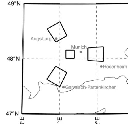
The wave vector is related to the intrinsic wave frequency, i.e. the frequency that would be observed in a frame of ref-erence moving with the horizontal background wind, via the Brunt–Väisälä frequency and the Coriolis parameter (disper-sion equation, see Eq. 38 in Fritts and Alexander, 2003). Based on the work of Wachter et al. (2015), we constructed a scanning OH∗ spectrometer (Sect. 2.1) which allows the derivation of periods and zonal as well as meridional wave-lengths (method: Sect. 3.1, and results: Sect. 4.1). We then use literature values of the Brunt–Väisälä frequency (see e.g. Wüst et al., 2016, 2017b) and the nearest mesopause wind measurements, which are performed by a meteor radar (Sect. 2.3) in order to estimate the vertical wavelengths (method: Sect. 3.1, and results: Sect. 4.2). The scanning spec-trometer operates at Oberpfaffenhofen (48.09◦N, 11.28◦E),
Germany, the meteor radar is deployed at Collm (51.30◦N,
13.02◦E), Germany, ca. 380 km northeast of Oberpfaffen-hofen; therefore, specific focus is put on a thorough uncer-tainty estimation (Sect. 3.2). Finally, the results are compared to vertical wavelengths extracted from collocated TIMED-SABER temperature profiles (Sects. 2.2, and 4.2).
Figure 1.The scanning GRIPS points in four different directions. The FoV in the zenith direction is the smallest one with an edge length of 23–24 km at the mesopause height resulting in a covered area of ca. 560 km2. The remaining three FoVs are larger (approxi-mately 880 km2). All four FoVs together form an equilateral trian-gle, whose sides are approximately 90 km long.
2 Measurements and data 2.1 Infrared spectrometer GRIPS
The nightly airglow observations presented here are per-formed with the scanning infrared spectrometer GRIPS 14 (Ground based Infrared P-branch Spectrometer) at Oberp-faffenhofen (48.09◦N, 11.28◦E), Germany, July–November 2015. The instrument operates in the spectral range of 1.5 to 1.6 µm. Therefore, observations are only possible under (nearly) cloudless conditions. They address a height of ca. 86 km (e.g. Wüst et al., 2016, 2017b).
anal-ysis, 5 min mean values are calculated for each FoV. Only comparatively good individual values are used here (individ-ual error 4.5 K and less as in Wüst et al., 2016). The error of the 5-minute values reaches ca. 3.2 K on average with a standard deviation of 0.3 K. Additional care has been taken to ensure that the data quality of each FoV is comparable to the others by manually inspecting each night: due to the geo-graphic location of Oberpfaffenhofen, just north of the Alps, clouds frequently form predominantly in the southern FoV or the moon passes through one of the FoVs. These cases are excluded from further analysis.
2.2 TIMED-SABER
On 7 December 2001, the TIMED satellite was launched. Soon, the on-board limb-sounder SABER started to deliver vertical profiles of kinetic temperature on a routine basis. The profiles cover the height range from approximately 10 km to more than 100 km. The vertical resolution is ca. 2 km (Mertens et al., 2004; Mlynczak, 1997), which is suitable for the investigation of gravity wave activity. On a given day, the latitudinal coverage extends from about 52◦ latitude in one hemisphere to 83◦ in the other (Russell et al., 1999). This viewing geometry alternates once every 60 days due to 180◦yaw manoeuvres of the TIMED satellite (Russell et al., 1999). In total, approximately 1200 temperature profiles are available per day. An overview of the large number of SABER publications is available at http://saber.gats-inc.com/ publications.php.
Measurements of infrared emission from carbon dioxide in the 15 µm spectral interval are used in the SABER tem-perature retrieval. It is based on a comprehensive forward radiance model incorporating dozens of vibration-rotation bands of CO2, including isotopic and hot bands, and solv-ing the full set of coupled radiative transfer equations under non-LTE, i.e. under conditions that depart from local ther-modynamic equilibrium. From the temperature retrieval ver-sion 1.03 on, NLTE algorithms for kinetic temperature were employed (López-Puertas et al., 2004; Mertens et al., 2004, 2008). This is certainly one of the main challenges for CO2 based temperature retrievals in the mesosphere and upper levels. Comparisons with reference data sets generally con-firm good quality of SABER temperatures (Remsberg et al., 2008).
We use nightly TIMED-SABER temperature data be-tween 45.4 and 50.8◦N and 8.6 and 14.0◦E (∼300 km dis-tance from Oberpfaffenhofen (48.09◦N, 11.28◦N)) in its
lat-est version (2.0). They were downloaded from the SABER homepage (http://saber.gats-inc.com). The exact time can be looked up in Table 1. Only SABER profiles that were mea-sured at the same time as GRIPS data series were used.
The data were detrended between 100 km and their height minimum using an iterative cubic spline approach as it is de-scribed in Wüst et al. (2017a) with a distance of 10 km be-tween two spline sampling points. This results in a maximal
detectable wavelength of 20 km (in the detrended data se-ries). We restrict further analysis to a relatively small height interval of 60–80 km which is just below the height range ad-dressed by GRIPS. This is due to the following reasons. Es-pecially during summer (May–August), a time period which is also covered in this study, the mesopause is low and reaches ca. 86 km±3 km (von Zahn et al., 1996; She et al., 2000). Sharply changing temperature gradients are always a challenge for a de-trending procedure and artificial signals in the detrended data cannot be excluded here. This is the rea-son why we investigate only heights below 80 km with the harmonic analysis. The majority of commonly used spec-tral analysis techniques like the fast fourier transform, the maximum entropy method and also the harmonic analysis approach, all assume the waves are stationary and therefore a constant wave amplitude. Alternative analyses suited for non-stationary time series like, the wavelet analysis, for ex-ample, often suffer from a relatively coarse spectral resolu-tion. Therefore, we restrict our analysis to the smallest possi-ble height interval which is equal to the maximal wavelength detectable in the detrended data series.
2.3 Meteor wind radar
The VHF SKiYMET meteor radar located at Collm has been operated nearly continuously since July 2004 (Jacobi et al., 2007, 2009). It measures winds, temperatures, and some me-teor parameters at altitudes between approximately 80 and 100 km.
The radar operates at a frequency of 36.2 MHz, with 15 kW peak power at a pulse repetition frequency of 625 Hz. The transmit antenna is a crossed dipole one, while the 5 re-ceiving antennas during 2015 were 2-element Yagi antennas, forming an interferometer to detect the meteor position.
The radar uses the Doppler shift of the reflected radio wave from ionized meteor trails to obtain radial velocities along the line of sight of the radio wave. Hourly mean horizontal wind values are obtained from a least squares fit of the pro-jection of the horizontal hourly wind components to all in-dividual radial winds within 1 h and within a defined height gate under the assumption that vertical winds are small. We used height gates of 4 km width for the fit, without weight-ing the individual meteors and assumweight-ing that the wind field within the time-height bin is homogeneous. Horizontal ho-mogeneity of the horizontal wind field within the radar ob-servation volume is also assumed. The procedure is described in Hocking et al. (2001). A more recent version of the wind fitting technique and error estimation of meteor radar winds can be found in Stober et al. (2017).
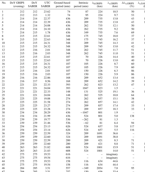
dur-Table 1.Ground-based periodT, intrinsic frequencyσ, vertical and horizontal wavelengths,λzand λh, as well as error of the vertical wavelength1λz, derived from GRIPS, and vertical wavelengthλz(if calculated) derived from SABER measurements during different nights (DoY=day of year when the measurement started), and date as well as time of the co-located SABER measurements.
No. DoY GRIPS DoY UTC Ground-based Intrinsic λh,GRIPS λz,GRIPS 1λz,GRIPS λz,SABER (evening) SABER SABER period (min) period (min) (km) (km) (%) (km)
1 212 212 23.62 74 87 224 10.5 50 12.6
2 212 213 1.32 74 95 224 9.7 53 8.1
3 214 214 22.37 436 209 735 13.8 43 11.0
4 214 214 22.39 436 209 735 13.8 43 14.5
5 214 214 24.08 436 262 735 12.1 50 7.0
6 214 214 24.10 436 262 735 9.2 50 9.0
7 214 215 1.78 436 349 735 7.6 69 8.7
8 215 215 22.61 348 175 745 18.0 37 11.2
9 215 215 22.63 348 175 745 16.2 37 12.1
10 215 215 24.31 348 209 745 14.3 41 15.7
11 215 215 24.32 348 209 745 13.0 42 7.2
12 215 216 2.01 348 262 745 11.7 51 12.7
13 215 216 2.03 348 262 745 11.0 51 12.4
14 215 215 22.61 107 70 226 14.4 40 11.2
15 215 215 22.63 107 70 226 13.0 40 12.1
16 215 215 24.31 107 105 226 8.7 60 9.1
17 215 215 24.32 107 105 226 7.9 60 7.2
18 215 216 2.01 107 150 226 6.3 86 8.2
19 215 216 2.03 107 150 226 5.9 86 7.1
20 216 216 22.86 168 209 652 13.4 44 15.9
21 216 217 0.56 168 209 652 14.2 39 16.1
22 221 221 22.33 393 262 823 13.2 47 14.5
23 221 221 24.04 393 1047 823 1.5 – –
24 221 221 22.33 148 131 525 19.1 36 14.5
25 221 221 24.04 148 262 525 10.8 64 8.9
26 225 225 19.88 274 262 857 15.1 38 8.7
27 225 225 21.58 274 262 857 14.1 42 9.8
28 225 225 23.27 274 209 857 17.4 33 10.9
29 225 225 23.28 274 209 857 18.3 33 12.4
30 234 234 20.29 436 −1047 801 1.9 – –
31 234 234 21.99 436 524 801 5.0 138 5.5
32 239 239 19.77 536 −262 81 1.3 – –
33 239 239 21.46 536 −62 81 6.4 94 9.4
34 254 254 23.13 626 524 657 5.8 117 5.3
35 254 254 23.14 626 524 657 5.5 116 3.6
36 259 259 22.59 324 209 1691 36.6 – –
37 259 259 22.60 324 209 1691 38.8 – –
38 259 259 22.59 200 209 421 8.3 71 8.5
39 259 259 22.60 200 209 421 8.8 71 11.7
40 263 263 21.82 608 524 1801 15.9 51 13.8
41 263 263 21.83 608 524 1801 14.0 51 17.4
42 275 275 19.53 616 – – imaginary – –
43 275 275 19.54 616 – – imaginary – –
44 275 275 19.53 158 116 634 44.6 – –
45 275 275 19.54 158 116 634 44.4 – –
46 284 285 3.51 557 −349 2054 7.8 95 5.4
47 284 285 3.51 257 150 436 33.4 – –
ing a half-year campaign in 2004/05 (Viehweg, 2006). The OSWIN radar had been operated as a meteor radar (Singer at al., 2003), with the same analysis procedure than applied at Collm. The Collm–Kühlungsborn differences were increas-ing from −0.7±22.3 m s−1 at 85 km to−2.5±25.5 m s−1 at 94 km for the zonal component, and −0.1±20.3 m s−1 at 85 km to−2.05±24.9 m s−1at 94 km for the meridional component. The small biases may be explained by the mean northward gradients of the horizontal winds, which at these heights in winter are positive for both the zonal and merid-ional wind components. The standard deviation is due to waves, turbulence, and uncertainties of both systems.
Therefore, when using Collm data for estimating winds over Oberpfaffenhofen, the standard deviation of about 20 m s−1may be considered as a good guess for the dynami-cally induced wind differences.
3 Analysis methods
3.1 Derivation of 3-D wave vector
The basic idea of the algorithm applied here for the calcu-lation of horizontal wavelengths from a scanning GRIPS in-strument is already mentioned in Wachter et al. (2015). In contrast to their publication, we derive OH-temperatures for four instead of three FoVs with one scanning GRIPS instru-ment instead of three individual (non-scanning) ones. Since three FoVs are sufficient for the calculation of horizontal wavelengths, we use the additional information for the es-timation of uncertainty intervals.
We apply the harmonic analysis (all-step mode, see for ex-ample Bittner et al., 1994, or Wüst and Bittner, 2006) to the four nightly time series and search for four identical (ground-based, not intrinsic) periods throughout the entire night. Fur-ther analysis steps are restricted to results which are charac-terized by a period longer (shorter) than 60 min (the measure-ment time) and an amplitude larger than or equal to 1 K. This is in accordance with the approach and the results of Wachter et al. (2015) (see their Sect. 2.2).
Since four different triangles can be derived from four dif-ferent FoVs, we apply the algorithm described in Wachter et al. (2015) to each possible triangle combination. So, we get information about the horizontal wavelengths λh(wave numberskh)from each of the four triangle combinations for four waves at maximum. Zonal and meridional wavelengths (numbers)λx(k)andλy(l), phase velocities, and propagation directions can be derived. The mean parameters are calcu-lated for each wave, and the mean absolute difference be-tween the individual values and the mean parameters are taken as a measure of uncertainty.
Since phase velocities reported in the literature do not in most cases exceed 150 m s−1 (e.g. Nakamura et al., 1999; Taylor et al., 2009; Tang et al., 2014; Wachter et al., 2015), only waves with a mean phase velocity of 150 m s−1at
maxi-mum and a mean horizontal wavelength of less than or equal to 3600 km are subject of further analysis. Additionally, a maximal difference of 90◦between the four different wave
vectors is accepted. It turned out that this criterion is the strictest one: if it is fulfilled, the others are met as well.
Going one step further than Wachter et al. (2015), we then use the dispersion relation for the estimation of vertical wavelengths. According to linear theory (see, for example, Fritts and Alexander, 2003), it holds the following:
m2= k
2+l2
N2−σ2
σ2−f2 −
1
4H2, (1)
wheremis the vertical wave number,Nis the Brunt–Väisälä frequency,σ=ω−ku−lvis the intrinsic frequency (the fre-quency that would be observed in a frame of reference mov-ing with the background wind(u, v)), ω is the frequency derived by the harmonic analysis, f =2· 2π
86 164 s·sinβ is the Coriolis parameter with respect to the latitudeβ, which reaches typically 10−4s−1 for mid-latitudes, and H is the density scale height.
For low- and medium-frequency waves (σ∼f or N σf )the dispersion relation simplifies to the following:
λz=
2·π·pσ2−f2
N·kh
(2)
=
2·π·
q
(ω−k·u−l·v)2−f2
N·kh
,
wherekhis the horizontal wave number (see Eq. 38 in Fritts and Alexander, 2003). The term 1
4H2 can be neglected since it is small compared to the squared vertical wave number. Due to the selection criteria for frequency and horizontal wave numbers,ω,k, andlare rather small and the use of this ap-proximation is justifiable.
Information about mesopause wind velocities above Oberpfaffenhofen is not available. Since tides, which are variable from day to day, play an important role in this height range, we do not rely on climatological wind values but make use of wind measurements performed with the wind meteor radar at Collm in order to estimate the intrinsic frequency.
Since GRIPS only measures the temperature at about 86 km height, but not the temperature gradient, the Brunt– Väisälä (angular) frequency is calculated based on the collo-cated TIMED-SABER measurements.
3.2 Error estimation
Sinceωis calculated using four different time series and ap-plying a variety of quality criteria, we argue that the error of
then sums up to the following:
1λz=
s
∂λ
z
∂k1k
2
+
∂λ
z
∂l 1l
2
+
∂λ
z
∂N1N
2
(3)
+
∂λ
z
∂u1u
2
+
∂λ
z
∂v 1v
2
,
with the following equations:
∂λz
∂k 1k= −λz·1k·
σ·u
σ2−f2+
k k2+l2
, (4)
∂λz
∂l 1l= −λz·1l·
σ·v
σ2−f2+
l
k2+l2
, (5)
∂λz
∂N1N= −λz·
1N
N , (6)
∂λz
∂u1u= −λz·
σ·k
σ2−f2·1u, (7)
∂λz
∂v 1v= −λz·
σ·l
σ2−f2·1v. (8)
Following Wüst et al. (2016) and Wüst et al. (2017b), 1NN is ca. 10 %. This might be overestimated, sinceN is calcu-lated from collocated TIMED-SABER profiles. However, the satellite-based measurements do not agree exactly in space with the GRIPS measurements. They represent only a snap-shot and analyses concerning the general temporal and spa-tial variability of N within 300 km are difficult due to the distance of individual TIMED-SABER profiles.1uand1v
are approximately 20 m s−1(see Sect. 2.3), and1k and1l
are estimated as stated above (see Sect. 3.1). Now,1λzan be calculated.
Errors which may arise due to tidal effects on the OH-layer height are not considered here. Strong tidal perturbations lead to airglow-altitude changes from typically 2–7 km (Zhao et al., 2005). If all four FoVs are affected to the same extent (the OH-airglow altitude is shifted by a constant value), our results are not influenced. If the OH-airglow layer height in-creases or dein-creases for each FoV individually, the derived horizontal wavelengths can change. However, our results rely on spatial and temporal averages. The FoVs cover 880 km2 (560 km2); all values which we derive are averaged over this area. Furthermore, we analyse time series of 7 h and longer. So, effects of motions of these scales cancel out. The four FoVs are rather near to each other. This reduces the possible effect of large scale motions like tides on our analysis results tremendously. Due to the redundancy of the system (we get four values for the horizontal wavelength), we dismiss results which do not agree sufficiently (as mentioned in Sect. 3.1). This might be the case when not all but only one or two FoVs are influenced by a higher or lower airglow altitude.
There is a secondary tidal effect. If the OH-airglow layer height disagrees significantly from 86 km, we use the wind information of the wrong altitude bin. Due to the width of the altitude bins, we might be one bin off in the case of strong
tidal perturbations as mentioned above. The error depends on the vertical wind shear. Placke et al. (2011) show histograms of the zonal and meridional wind shear values (prevailing and tidal wind) for the years 2005–2009 referring to July mea-sured by the radar at Collm. On average, the zonal (merid-ional) wind shear is ca. 5 m s−1km−1(0 m s−1km−1). So if we are one bin off, this is equivalent to 20 m s−1. This agrees with the error which we assumed for each wind component.
4 Results and discussion 4.1 Horizontal parameters
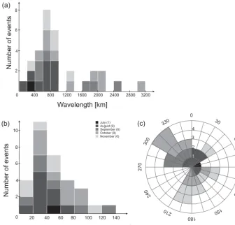
Due to the rather strict quality criteria, horizontal wave-lengths for 31 wave events in only 22 nights can be identified during the measurement period. For the majority of cases, the horizontal wavelength is shorter than 1000 km, with a max-imum of the distribution between 600 and 800 km (Fig. 2a). The phase velocity (relative to the ground) reaches 140 m s−1 at maximum and ranges mostly between 20 and 40 m s−1 (Fig. 2b). A preferred propagation direction cannot easily be identified (Fig. 2c). The data cover the time period from July to November; since the propagation direction is supposed to show seasonal variations (see Wachter et al., 2015, and refer-ences therein) and our data base is rather small, a conclusive picture cannot be drawn here.
The values for the different parameters agree well with lit-erature. Phase velocities up to 80–100 m s−1are reported, for example, by Nakamura et al. (1999), Suzuki et al. (2004), and Taylor et al. (2009). For example, Tang et al. (2014) and Wachter et al. (2015) find horizontal phase speeds of up to 160–180 m s−1. The horizontal wavelengths cannot easily be compared since many authors focus on smaller horizon-tal scales (see, for example, Tang et al., 2014; Taylor et al., 2009; Hannawald et al., 2016; Sedlak et al., 2016). However, Reid (1986) presents in his Fig. 6a good overview of horizon-tal wavelengths measured by different techniques at various locations between 60 and 100 km height. Here, it becomes clear that horizontal wavelengths of the order of 103km were already observed in earlier studies. However, in order to be careful, the results of the following subsection are separated according to the horizontal wavelength (up to 1500 km and all wavelengths, provided in brackets if the results disagree). 4.2 Vertical wavelengths
8
6
4
2
July (1) August (9) September (6) October (9) November (6)
0 400 800 1200 1600 2000 2400 2800 3200
Wavelength [km]
Number of events
20 40 60 80 100 120 140
Phase velocity(relative to the ground)[m s-1]
10
8
6
4
2
0
Number of events
0
30
60
90
12
0
150
180
210 24 0
27
0
300
330
4 3
2
1
Azimuth [°] (a)
(b) (c)
Figure 2.The histogram of the horizontal wavelengths(a)shows that the majority of detected wave events reaches up to 1000 km. The distribution of phase velocities (relative to the ground)(b)is smoother and has a maximum between 20 and 40 m s−1. The diagram of horizontal propagation directions(c)does not show a conclusive picture. The different grey colours refer to the different months.
wavelengths, can be used for comparison. Since the wind velocity changes considerably during the night, we calcu-late linearly weighted wind speeds from the hourly means of the wind data according to the overflight time of TIMED. If multiple nearby SABER profiles are available, the detected wave from the airglow is combined with different wind val-ues. This leads to different vertical wavelengths based on the GRIPS-radar combination for one night. In one case, the re-spective hourly averaged wind data do not exist. Therefore, 19 horizontal wavelengths of the 31 mentioned in Sect. 4.1 referring to 14 of 22 nights can be used for further analysis. The data availability of TIMED-SABER and meteor wind measurements allows the calculation of 48 vertical wave-lengths (see Table 2).
In three cases, the wavelengths are shorter than 2 km (no. 23, 30 and 32 in Table 1). This does not seem to be a realis-tic value for a layer with a full width at half maximum of 8– 9 km (see Fig. 9 in Wüst et al., 2016, 2017b). Furthermore, as Trinh et al. (2015) show in their Fig. 7a, SABER is not sensi-tive for vertical wavelengths shorter than ∼2.5 km. In five cases (twice two nearly simultaneously measured SABER profiles), the wavelengths are rather long with ca. 38.0 km
(no. 36 and 37 in Table 1), 45.9 km (no. 44 and 45 in Ta-ble 1) and 33.4 km (no. 47 in TaTa-ble 1). This is in principle possible and was already observed in the past (see, for exam-ple, Manson, 1990, and Stober et al., 2013) but hard to ver-ify here since we use SABER profiles only between 60 and 80 km – see Sect. 2.2 for an explanation. In two cases (two nearly simultaneously measured SABER profiles), the result is imaginary (no. 42 and 43 in Table 1), which means that the wave cannot propagate vertically. We cannot verify this case either. So, 38 cases (79 % of 48 vertical wavelengths) show reasonable and verifiable results.
measure-0 2 4 6 8 10 12
5 7 9 11 13 15 17 19 21
Number
of
ev
en
ts
λz, GRIPS[km]
14
(a)
(b)
0 2 4 6 8 10 12
30 40 50 60 70 80 90 100 > 100
Number
of
ev
en
ts
Δλz, GRIPS[%]
Figure 3.The mean calculated vertical wavelength is ca. 11.6 km, while the individual values spread from 5 to 19–20 km(a), thexaxis labels are the upper limits of the respective intervals. The mean er-ror of the vertical wavelength1λzbased on error propagation cal-culations reaches ca. 59 %(b). At minimum, it ranges between 30 and 40 %; in three cases, it is more than 100 %. The values for the waves with horizontal wavelengths larger than 1500 km are marked in light grey.
ments, they find that characteristic vertical wavelengths vary between 8.9 and 27 km. The annual mean reaches 14.1 km if one refers only to summer values, it is 12.7 km, winter values show a mean of 15.5 km.
The mean error following Eq. (3) sums up to 59 % (Fig. 3b). In nearly all cases, the largest contribution to the individual1λzis due to the wind uncertainty (Eqs. 7 and 8). In order to compare the vertical wavelengths derived by GRIPS with SABER measurements, the harmonic analysis is used for searching the detrended TIMED-SABER temper-ature profiles for two vertical wavelengths between 2.5 km (minimal vertical wavelengths detectable in SABER mea-surements according to Trinh et al., 2015) and 20 km (height interval length). Two wavelengths are chosen since an in-spection shows at least two oscillations in the SABER pro-files. The sensitivity of TIMED-SABER depends on the ver-tical and horizontal wavelength along the line of sight. For a wave with 12.5 km vertical wavelength, the horizontal
wave-12 0 2 4 6 8 10 12
1 2 3 4 5 6 7 > 8
Number
of
ev
en
ts
(a)
(b)
[km] |λz, GRIPS- λz,SABER|
0 2 4 6 8 10
10 20 30 40 50 > 60
Number
of
ev
en
ts
|λz, GRIPS- λz,SABER|[%]
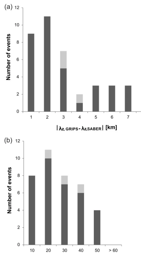
Figure 4.The mean difference between the vertical wavelength de-rived by the scanning GRIPSλz,GRIPSand the most similar vertical wavelength identified in collocated TIMED-SABER vertical tem-perature profilesλz,SABERis ca. 2.5 km(a)or 21 %(b). It reaches 6–7 km or 40–50 % at maximum.
length (along the line of sight) needs to be 450 km at least, to ensure that SABER captures it with 50 % and more of its original amplitude (see Trinh et al., 2015, for example). The horizontal wavelength along the line of sight is always larger or equal to the true horizontal wavelength. The TIMED-SABER data are therefore suitable for our purpose (compare Fig. 2a).
mean individual difference between the vertical wavelengths of both data sets then reaches ca. 2.5 km or 21 % relative to the GRIPS wavelength (Fig. 4a and b). The vertical wave-lengths agree within the error bars in all but four cases; here, the vertical wavelengths derived from SABER are slightly smaller by 0.2–0.8 km.
We conclude that the presented approach provides reason-able results for the 3-D wave vector. However, the data basis is not very large. Like other measurement techniques or ap-proaches, this one is also sensitive to certain horizontal and vertical wavelengths: the vertical extension of the OH∗-layer limits the sensitivity of the GRIPS-instrument for vertical wavelengths to a few kilometres at least (see Wüst et al., 2016 for a comprehensive overview). The sensitivity for horizon-tal wavelengths is determined by the distance between the different FoVs (∼90 km here) and their sizes (see Wüst et al., 2016, for an estimation of this effect), as well as by the quality of the data, which strongly depends on the weather: only if a phase difference unequal to zero for the individual time series can be identified, the derivation of the horizontal wave vector and subsequently of the vertical wave number is possible.
5 Summary
Using a scanning OH-spectrometer at Oberpfaffenhofen (48.09◦N, 11.28◦E), Germany, we derive periods and hor-izontal wavelengths at the mesopause which are typi-cal for gravity waves (ca. 1–10 h, 100–1000s km). Based on the dispersion relation, additional horizontal wind in-formation allows the calculation of vertical wavelengths. The nearest mesopause wind measurements are carried out at Collm (51.30◦N, 13.02◦E), Germany, approximately 380 km northeast of Oberpfaffenhofen by a meteor radar. We assume that these values are also valid for Oberpfaffenhofen within an uncertainty of±20 m s−1.
Ca. 79 % of the vertical wavelengths range between 5 km and 19–20 km. These values appear reasonable compared to literature and taking into account the vertical extension of the OH-layer. In three cases (ca. 6 %), the values are not plausi-ble.
The results are compared to vertical wavelengths derived from collocated detrended TIMED-SABER measurements. Although the spectrometer and the meteor radar are deployed about 380 km apart from each other, the vertical wavelengths based on the spectrometer-radar data combination and the satellite data only show a mean difference of 2.5 km or 21 % (relative to the GRIPS wavelength). We conclude that the presented combination of measurements provides a good es-timate of the vertical wavelengths on average.
Data availability. The SABER data are available at the SABER homepage http://saber.gats-inc.com/data. php (SABER, 2018). The NDMC are available at https://doi.org/10.1594/WDCRSAT.R4OAR50I (Offenwanger et al., 2018). Collm hourly radar wind data are available from Christoph Jacobi upon request.
Competing interests. The authors declare that they have no conflict of interest.
Acknowledgements. We thank the Bavarian State Ministry of the Environment and Consumer Protection (BayStMinUV, VAO-project LUDWIG, TP I/3, VAO-project number TUS01 UFS-67093) and the German Ministry for Education and Research (BMBF, Grant agreement No: 01LG1206A) for funding.
Furthermore, we thank Ricarda Linz, formerly at DLR, for de-trending the SABER data and Paul Wachter, DLR, for a preliminary setup of the scanning GRIPS-instrument.
Processing and long-term archiving of the data is provided by the World Data Center for Remote Sensing of the Atmosphere (WDC-RSAT, http://wdc.dlr.de). The measurements are part of the Network for the Detection of Mesospheric Change, NDMC (https: //www.wdc.dlr.de/ndmc).
Finally, we thank the reviewers for their valuable comments.
The article processing charges for this open-access publication were covered by a Research
Centre of the Helmholtz Association.
Edited by: William Ward
Reviewed by: Alan Liu and two anonymous referees
References
Bittner, M., Offermann, D., Bugaeva, I. V., Kokin, G. A., Koshelkov, J. P., Krivolutsky, A., Tarasenko, D. A., Gil-Ojeda, M., Hauchecorne, A., Lübken, F.-J., de la Morena, B. A., Mourier, A., Nakane, H., Oyama, K. I., Schmidlin, F. J., Soule, I., Thomas, L., and Tsuda, T.: Long period/large scale oscilla-tions of temperature during the DYANA campaign, J. Atmos. Sol.-Terr. Phys., 56, 1675–1700, https://doi.org/10.1016/0021-9169(94)90004-3, 1994.
Bittner, M., Offermann, D., and Graef, H.-H.: Mesopause tempera-ture variability above a midlatitude station in Europe, J. Geophys. Res., 105, 2045–2058, 2000.
Chen, C., Chu, X., Zhao, J., Roberts, B. R., Yu, Z., Fong, W., Lu, X., and Smith, J. A.; Lidar observations of persistent gravity waves with periods of 3–10 h in the Antarctic middle and up-per atmosphere at McMurdo (77.83◦S, 166.67◦E), J. Geophys. Res.-Space, 121, 1483–1502, 2016.
Fritts, D. C. and Alexander, M. J.: Gravity wave dynamics and effects in the middle atmosphere, Rev. Geophys., 41, 1003, https://doi.org/10.1029/2001RG000106, 2003.
Garcia, F. J., Taylor, M. J., and Kelly, M. C.: Two-dimensional spec-tral analysis of mesospheric airglow image data, Appl. Opt., 36, 7374–7385, https://doi.org/10.1364/AO.36.007374, 1997. Hannawald, P., Schmidt, C., Wüst, S., and Bittner, M.: A fast SWIR
imager for observations of transient features in OH airglow, At-mos. Meas. Tech., 9, 1461–1472, https://doi.org/10.5194/amt-9-1461-2016, 2016.
Hocking, W. K., Fuller, B., and Vandepeer, B.: Real-time deter-mination of meteor-related parameters utilizing modern digi-tal technology, J. Atmos. Sol.-Terr. Phys., 63, 155–169, 2001, https://doi.org/10.1016/S1364-6826(00)00138-3, 2001. Jacobi, Ch., Fröhlich, K., Viehweg, C., Stober, G., and
Kürschner, D.: Midlatitude mesosphere/lower thermo-sphere meridional winds and temperatures measured with Meteor Radar, Adv. Space Res., 39, 1278–1283, https://doi.org/10.1016/j.asr.2007.01.003, 2007.
Jacobi, Ch., Arras, C., Kürschner, D., Singer, W., Hoffmann, P., and Keuer, D.: Comparison of mesopause region meteor radar winds, medium frequency radar winds and low fre-quency drifts over Germany, Adv. Space. Res., 43, 247–252, https://doi.org/10.1016/j.asr.2008.05.009, 2009.
Latteck, R., Singer, W., and Höffner, J.: Mesosphere Summer Echoes as observed by VHF Radar at Küh-lungsborn 54◦N, Geophys. Res. Lett., 26, 1533–1536, https://doi.org/10.1029/1999GL900225, 1999.
López-Puertas, M., Garcia-Comas, M., Funke, B., Picard, R. H., Winick, J. R., Wintersteiner, P. P., Mlynczak, M. G., Mertens, C. J., Russell III, J. M., and Gordley, L. L.: Evidence for an OH(v) excitation mechanism of CO24.3 µm nighttime emission from SABER/TIMED measurements, J. Geophys. Res., 109, D09307, https://doi.org/10.1029/2003JD004383, 2004.
Mertens, C. J., Schmidlin, F. J., Goldberg, R. A., Remsberg, E. E., Pesnell, W. D., Russell III, J. M., Mlynczak, M. G., López-Puertas, M., Wintersteiner, P. P., Picard, R. H., Winick, J. R., and Gordley, L. L.: SABER observations of mesospheric tempera-tures and comparisons with falling sphere measurements taken during the 2002 summer MaCWAVE campaign, Geophys. Res. Lett., 31, L03105, https://doi.org/10.1029/2003GL018605, 2004. Mertens, C. J., Fernandez, J. R., Xu, X., Evans, D. S., Mlynczak, M. G., and Russell III, J. M.: A new source of auroral infrared emission observed by TIMED/SABER, Geophys. Res. Lett., 35, 17–20, https://doi.org/10.1029/2008GL034701, 2008.
Mlynczak, M. G.: Energetics of the mesosphere and lower thermo-sphere and the SABER experiment, Adv. Space Res., 20, 1177– 1183, https://doi.org/10.1016/S0273-1177(97)00769-2, 1997. Mulligan, F. J., Horgan, D. F., Galligan, J. G., and Griffin, E.
M.: Mesopause temperatures and integrated band brightnesses calculated from airglow OH emissions recorded at Maynooth (53.2◦N, 6.4◦W) during 1993, J. Atmos. Sol.-Terr. Phys., 57, 1623–1637, 1995.
Mzé, N., Hauchecorne, A., Keckhut, P., and Thétis, M.: Vertical distribution of gravity wave potential energy from long-term Rayleigh lidar data at a northern mid-dle latitude site, J. Geophys. Res., 119, 12069–12083, https://doi.org/10.1002/2014JD022035, 2014.
Nakamura, T., Higashikawa, A., Tsuda, T., and Matsushita, Y.: Sea-sonal variations of Gravity wave structures in OH airglow with a CCD imager at Shigaraki, Earth Planets Space, 51, 897–906, https://doi.org/10.1186/BF03353248, 1999.
Offenwanger, T., Schmidt, C., Wüst, S., and Bittner, M.: Five minute means of OH(3-1) airglow rotational temperatures from the mesopause region obtained with GRIPS 14 located at the German Remote Sensing Data Center, Oberpfaffenhofen, https://doi.org/10.1594/WDCRSAT.R4OAR50I, 2018.
Oleynikov, A. N., Jacobi, Ch., and Sosnovchik, D. M.: Parame-ters of internal gravity waves in the mesosphere-lower thermo-sphere region derived from meteor radar wind measurements, Ann. Geophys., 23, 3431–3437, https://doi.org/10.5194/angeo-23-3431-2005, 2005.
Paulino, I., Takahashi, H., Medeiros, A. F., Wrasse, C. M., Buriti, R. A., Sobral, J. H. A., and Gobbi, D.: Mesospheric gravity waves and ionospheric plasma bubbles observed during the COPEX campaign, J. Atmos. Sol.-Terr. Phys., 73, 1575–1580, 2011. Placke, M., Stober, G., and Jacobi, C.: Gravity wave momentum
fluxes in the MLT–Part I: Seasonal variation at Collm (51.3◦N, 13.0◦E), J. Atmos. Sol.-Terr. Phys., 73, 904–910, 2011. Rauthe, M., Gerding, M., Höffner, J., and Lübken, F.-J.:
Li-dar temperature measurements of gravity waves over Kühlungsborn (54◦N) from 1 to 105 km: A winter-summer comparison, J. Geophys. Res., 111, D24108, https://doi.org/10.1029/2006JD007354, 2006.
Rauthe, M., Gerding, M., and Lübken, F.-J.: Seasonal changes in gravity wave activity measured by lidars at mid-latitudes, Atmos. Chem. Phys., 8, 6775–6787, https://doi.org/10.5194/acp-8-6775-2008, 2008.
Reid, I. M.: Gravity wave motions in the upper middle atmo-sphere (60–110 km), J. Atmos. Sol.-Terr. Phys., 48, 1057–1072, https://doi.org/10.1016/0021-9169(86)90026-7, 1986.
Remsberg, E. E., Marshall, B. T., Garcia-Comas, M., Krueger, D., Lingenfelser, G. S., Martin-Torres, J., Mlynczak, M. G., Russell III, J. M., Smith, A. K., Zhao, Y., Brown, C., Gordley, L. L., Lopez-Gonzalez, M. J., Lopez-Puertas, M., She, C.-Y., Taylor, M. J., and Thompson, R. E.: Assessment of the quality of the ver-sion 1.07 temperature versus pressure profiles of the middle at-mosphere from TIMED/SABER, J. Geophys. Res., 113, D17101, https://doi.org/10.1029/2008JD010013, 2008.
Russell III, J. M., Mlynczak, M. G., Gordley, L. L., Tansock Jr., J. J., and Esplin, R. W.: Overview of the SABER experiment and preliminary calibration results, Proc. SPIE 3756, Optical Spec-troscopic Techniques and Instrumentation for Atmospheric and Space Research III, 277–288, https://doi.org/10.1117/12.366382, 1999.
SABER: SABER dataset, available at: http://saber.gats-inc.com/ data.php (28 October 2015), 2018.
Schmidt, C., Höppner, K., and Bittner, M.: A ground-based spectrometer equipped with an InGaAs array for rou-tine observations of OH(3-1) rotational temperatures in the mesopause region, J. Atmos. Sol.-Terr. Phys., 102, 125–139, https://doi.org/10.1016/j.jastp.2013.05.001, 2013.
Sedlak, R., Hannawald, P., Schmidt, C., Wüst, S., and Bittner, M.: High-resolution observations of small-scale gravity waves and turbulence features in the OH airglow layer, Atmos. Meas. Tech., 9, 5955–5963, https://doi.org/10.5194/amt-9-5955-2016, 2016. Senft, D. C. and Gardner, C. S.: Seasonal variability of
gravity wave activity and spectra in the mesopause re-gion at Urbana, J. Geophys. Res., 96, 17229–17264, https://doi.org/10.1029/91JD01662, 1991.
She, C. Y., Chen, S., Hu, Z., Sherman, J., Vance, J. D., Vasoli, V., White, M. A., Yu, J., and Krueger, D. A.: Eight-year climatology of nocturnal temperature and sodium density in the mesopause region (80 to 105 km) over Fort Collins, Co (41◦N, 105◦W), Geophys. Res. Lett., 27, 3289–3292, 2000.
Singer, W., Bremer, J., Hocking, W. K., Weiß, J., Latteck, R., and Zecha M.: Temperature and wind tides around the sum-mer mesopause at middle and Arctic latitudes, Adv. Space Res., 31, 2055–2060, https://doi.org/10.1016/S0273-1177(03)00228-X, 2003.
Stober, G., Sommer, S., Rapp, M., and Latteck, R.: Investi-gation of gravity waves using horizontally resolved radial velocity measurements, Atmos. Meas. Tech., 6, 2893–2905, https://doi.org/10.5194/amt-6-2893-2013, 2013.
Stober, G., Matthias, V., Jacobi, C., Wilhelm, S., Höffner, J., and Chau, J. L.: Exceptionally strong summer-like zonal wind rever-sal in the upper mesosphere during winter 2015/16, Ann. Geo-phys., 35, 711–720, https://doi.org/10.5194/angeo-35-711-2017, 2017.
Suzuki, S., Shiokawa, K., Otsuka, Y., Ogawa, T., and Wilkinson, P.: Statistical characteristics of gravity waves observed by an all-sky imager at Darwin, Australia, J. Geophys. Res., 109, D20S07, https://doi.org/10.1029/2003JD004336, 2004.
Tang, Y., Dou, X., Li, T., Nakamura, T., Xue, X., Huang, C., Man-son, A., Meek, C., Thorsen, D., and Avery, S.: Gravity wave char-acteristics in the mesopause region revealed from OH airglow imager observations over Northern Colorado, J. Geophys. Res.-Space, 119, 630–645, https://doi.org/10.1002/2013JA018955, 2014.
Taylor, M. J., Pendleton Jr., W. R., Seo, S. H., and Picard, R. H.: Remote sensing of gravity wave intensity and temperature signa-tures at mesopause heights using the nightglow emissions, Proc. SPIE, 4882, 122–133, 2003.
Taylor, M. J., Pautet, P.-D., Medeiros, A. F., Buriti, R., Fechine, J., Fritts, D. C., Vadas, S. L., Takahashi, H., and São Sabbas, F. T.: Characteristics of mesospheric gravity waves near the magnetic equator, Brazil, during the SpreadFEx campaign, Ann. Geophys., 27, 461–472, https://doi.org/10.5194/angeo-27-461-2009, 2009.
Trinh, Q. T., Kalisch, S., Preusse, P., Chun, H.-Y., Eckermann, S. D., Ern, M., and Riese, M.: A comprehensive observational filter for satellite infrared limb sounding of gravity waves, Atmos. Meas. Tech., 8, 1491–1517, https://doi.org/10.5194/amt-8-1491-2015, 2015.
Viehweg, C.: Statistische Analyse von Meteorradardaten, Diploma Thesis, University of Leipzig, 86 pp., 2006.
von Savigny, C., McDade, I. C., Eichmann, K.-U., and Bur-rows, J. P.: On the dependence of the OH∗ Meinel emis-sion altitude on vibrational level: SCIAMACHY observations and model simulations, Atmos. Chem. Phys., 12, 8813–8828, https://doi.org/10.5194/acp-12-8813-2012, 2012.
von Zahn, U., Höffner, J., Eska, V., and Alpers, M.: The mesopause altitude: Only two distinctive levels worldwide?, Geophys. Res. Lett., 23, 3231–3234, 1996.
Wachter, P., Schmidt, C., Wüst, S., and Bittner, M.: Spatial grav-ity wave characteristics obtained from multiple OH(3–1) airglow temperature time series, J. Atmos. Sol.-Terr. Phys., 135, 192– 201, https://doi.org/10.1016/j.jastp.2015.11.008, 2015.
Wüst, S. and Bittner, M.: Non-linear resonant wave–wave interac-tion (triad): Case studies based on rocket data and first appli-cation to satellite data. J. Atmos. Sol.-Terr. Phys., 68, 959–976, https://doi.org/10.1016/j.jastp.2005.11.011, 2006.
Wüst, S., Wendt, V., Schmidt, C., Lichtenstern, S., Bittner, M., Yee, J.-H., Mlynczak, M. G., and Russell III, J. M.: Derivation of gravity wave potential energy density from NDMC measurements, J. Atmos. Sol.-Terr. Phys., 138, 32–46, https://doi.org/10.1016/j.jastp.2015.12.003, 2016.
Wüst, S., Wendt, V., Linz, R., and Bittner, M.: Smoothing data series by means of cubic splines: quality of approximation and intro-duction of a repeating spline approach, Atmos. Meas. Tech., 10, 3453–3462, https://doi.org/10.5194/amt-10-3453-2017, 2017a. Wüst, S., Bittner, M., Yee, J.-H., Mlynczak, M. G., and
Rus-sell III, J. M.: Variability of the Brunt–Väisälä frequency at the OH* layer height, Atmos. Meas. Tech., 10, 4895–4903, https://doi.org/10.5194/amt-10-4895-2017, 2017b.
Yamashita, C., Chu, X., Liu, H.-L., Espy, P. J., Nott, G. J., and Huang, W.: Stratospheric gravity wave characteris-tics and seasonal variations observed by lidar at the South Pole and Rothera, Antarctica, J. Geophys. Res., 114, D12101, https://doi.org/10.1029/2008JD011472, 2009.