https://doi.org/10.5194/npg-26-445-2019 © Author(s) 2019. This work is distributed under the Creative Commons Attribution 4.0 License.
A fast approximation for 1-D inversion of transient electromagnetic
data by using a back propagation neural network and improved
particle swarm optimization
Ruiyou Li, Huaiqing Zhang, Nian Yu, Ruiheng Li, and Qiong Zhuang
The State Key Laboratory of Transmission Equipment & System Safety and Electrical New Technology, Chongqing University, Chongqing, 400044, China
Correspondence:Huaiqing Zhang ([email protected]) Received: 22 June 2019 – Discussion started: 2 July 2019
Revised: 22 October 2019 – Accepted: 24 October 2019 – Published: 26 November 2019
Abstract. As one of the most active nonlinear inversion methods in transient electromagnetic (TEM) inversion, the back propagation (BP) neural network has high efficiency because the complicated forward model calculation is un-necessary in iteration. The global optimization ability of the particle swarm optimization (PSO) is adopted for amending the BP’s sensitivity to its initial parameters, which avoids it falling into a local optimum. A chaotic-oscillation iner-tia weight PSO (COPSO) is proposed for accelerating con-vergence. The COPSO-BP algorithm performance is vali-dated by two typical testing functions, two geoelectric mod-els inversions and a field example. The results show that the COPSO-BP method is more accurate, stable and needs rela-tively less training time. The proposed algorithm has a higher fitting degree for the data inversion, and it is feasible to use it in geophysical inverse applications.
1 Introduction
The transient electromagnetic (TEM) method applies the sec-ondary receiving voltage induced by the rapid switching of pulse current, and it then deduces the geoelectrical parame-ters consisting of the resistivities and thicknesses of the lay-ers. The later is a typical TEM inversion issue with nonlinear features. The linear inversion method was simple and widely used through linearization processes, yet it is extremely de-pendent on the selection of initial parameters and results in poor inversion accuracy. Hence, the nonlinear inversion
methods have attracted more geophysicists’ attention in re-cent years.
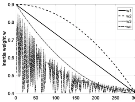
interpre-Figure 1.Inertial weight curves comparison.
tation for its powerful fitting ability. However, the neural-network method is sensitive to its initial parameter settings and falls easily into a local minimum. Many improved meth-ods were proposed for balancing the convergence rate and inversion quality. Zhang and Liu (2011) proposed ant colony optimization for ANN, and they applied high-density resis-tivity and acquired smaller inversion errors and higher deter-minant coefficients. Dai et al. (2014) suggested a differen-tial evolution (DE) for BP which enhanced the global search ability. Rosas-Carbajal et al. (2014) introduced the genetic algorithm for ANN.
The particle swarm optimization (PSO) has a simple struc-ture, fast convergence rate, high accuracy and global op-timization ability. Fernández et al. (2010) successfully in-troduced the PSO in a 1-D resistivity inversion. Godio and Santilano (2018) applied it in a geophysical inversion and deduced a depth resistivity earth model. Due to the PSO’s global searching performance, the BP’s initial weights and thresholds can be trained by the PSO, and the BP’s global optimization ability can be improved. Compared to the stan-dard PSO (SPSO), a chaotic-oscillation inertia weight PSO (COPSO) can accelerate the convergence rate in the early stage, and it was proposed naturally (Shi et al., 2009).
The paper structure is as follows: the principles of the PSO algorithm with different inertia weights schemes, the BP neural network and the proposed COPSO-BP algorithm are given in Sect. 2. Then, the COPSO-BP algorithm perfor-mance is validated by two typical testing functions in Sect. 3. And in a later section, inversion simulations of three-layer and five-layer geoelectric models are carried out; the hidden-layer neuron numbers determining method is put forward; and algorithm performance is compared.
Figure 2.Three-layer BP neural-network structure.
2 Principle of COPSO-BP algorithms 2.1 Chaotic-oscillation PSO algorithm
For ann-dimensional optimization problem, it is supposed that the position (resistivity and thickness for layered-model parameter inversion) and velocity (update speed) of theith particle (global search group number) at timetarexi=(xi1, xi2, . . . ,xiN) andvi=(vi1,vi2, . . . ,viN), respectively. Then, at timet+1, they can be calculated by the iterations as vidt+1=ω·vidt +c1r1(pidt −x
t
id)+c2r2(ptgd−x t
id), (1)
xidt+1=xidt +vtid+1, (2)
wherer1andr2are random values evenly distributed in the interval (0,1),c1andc2are learning factors (usually equal to 2), andpidandpgd are the individual and global maximum values.
The inertia weight parameterωaffects the algorithm per-formance seriously. A fixed weight always was used in the early time, and then various dynamic weights were proposed. Shi et al. (2010) have summarized several methods as ω1(t )=ωs−(ωs−ωe)t /Tmax, (3) ω2(t )=ωs−(ωs−ωe)(t /Tmax)2, (4) ω3(t )=ωs−(ωs−ωe)
h
2t /Tmax−(t /Tmax)2 i
, (5)
whereωsandωeare the start and end weight. ThetandTmax are the current and maximum iterations. The above weights are smooth and monotonically decreasing. In this paper, we proposed a decreasing oscillation weight scheme which was based on the chaotic logistic equation. Its specific calculation formula is
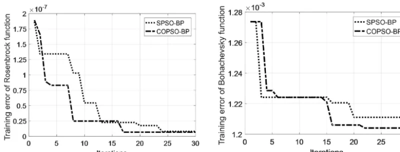
Figure 3.Training error curves of the SPSO-BP and COPSO-BP algorithms.
then obtained from Eq. (7). Numerical experiments were car-ried out correspondingly and showed that the initial value of x0 has little effect on the inertia weight ω. The inertia weight comparison was shown in Fig. 1, where x0=0.234 andµ=4 for chaotic oscillation.
2.2 BP neural network
The BP neural network has a multi-layer feed-forward struc-ture, and a typical three-layer network is shown in Fig. 2 (Li et al., 2009).
For Fig. 2,x1, x2, . . . ,xn are the input values,y1,y2, . . . , ymare the predicted outputs, andwijandwj kare the network weights. The threshold parameterαis defined in the hidden layer with its output,
Hj=f n X
i=1
wijxi−αj !
j=1,2, . . ., l, (8)
wherelis the hidden-layer node numbers,f is the activation function with different expressions, and the most widely used is a sigmoid-type function. The predicted output for thekth unit is calculated by
Ok= l X
j=1
Hjwj k−bk, (9)
and parameterbis the output threshold. Then the prediction error can be determined based on the predicted output Ok and the expected outputTk, which isek=(Tk−Ok)Ok(1− Ok). The updated formula for weights and thresholds is the following:
wij=wij+ηHj(1−Hj)xiPmk=1wj kek wj k=wj k+ηHjek
αj=αj+ηHj(1−Hj)Pmk=1wj kek bk=bk+ek
, (10)
whereiis 1,2, . . . ,n, j is 1,2, . . . ,l,kis 1,2, . . . ,mandηis the learning rate.
2.3 BP neural network with the COPSO algorithm The initial parameters are chosen randomly, which affects the convergence rate, learning efficiency and perhaps falling into a local minimum. The chaotic-oscillation PSO (COPSO) has a much better global optimization capability; therefore, the COPSO algorithm is proposed to optimize the initial weight and threshold of the BP. The COPSO-BP pseudo-codes are briefly described in Algorithm 1.
The formula for calculating theith particle fitness is de-fined as
fi= 1 S
S X
s=1 m X
j=1
Ysj− ˆYsj 2
, (11)
whereSis the number of training set samples,mis the output neurons number,Ysjis thejth true output of thesth sample, andYˆsj is the corresponding predicted output.
3 Algorithm testing
In order to investigate the COPSO-BP performance and reli-ability, Rosenbrock and Bohachevsky testing functions were adopted, which are typical non-convex functions and mainly evaluate the performance of unconstrained algorithms. How-ever, due to the random nature of the function, it is not easy to solve and has a global minimum function value of zero. 3.1 Rosenbrock function
f1(x)=100×
x12−x2 2
+(1−x1)2, xi
∈[−10,10], i=1,2 (12) 3.2 Bohachevsky function
f2(x)=x12+x23−x1x2x3+x3−sin
x22
−cosx1x32
Using the standard PSO-BP (SPSO-BP) with linear decreas-ing inertia weight in Eq. (3), the COPSO-BP tests were car-ried out. The three-layer BP with an n-s-1 structure is con-structed with different hidden nodes. The PSO parameters are the population sizeM=60, learning factors c1=c2= 2.0, maximum iterationTmax=30, inertia weightωs=0.9, ωe=0.4,x0=0.234 andµ=4 for chaotic parameters, and the search dimensionD=n×s+s×1+s+1, which includes all the neuron weights and thresholds. For BP network, 150 training samples and 50 testing samples were randomly pro-duced within the variable range. The training error is defined as
E= 1
S S X
s
(Ts−Os)2, (14)
whereSis the training samples number andTsandOsare the expected and predicted outputs for training samples, respec-tively. The network structures with minimum training errors for the Rosenbrock and Bohachevsky functions are 2-7-1 and
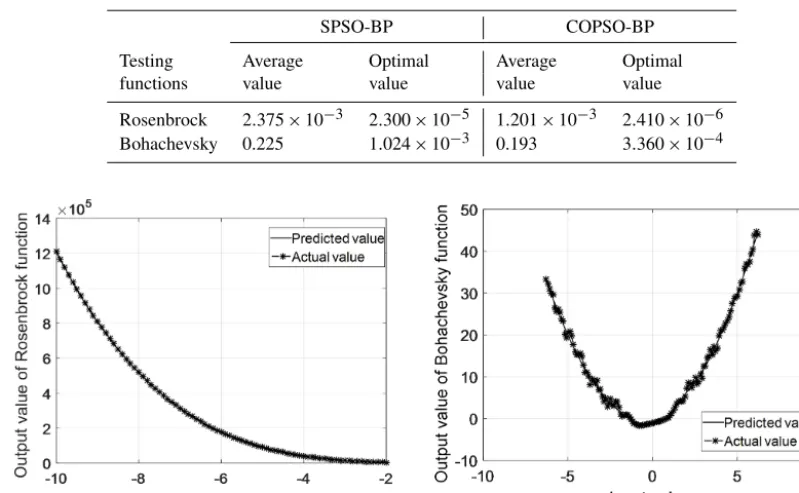
3-6-1, respectively. The simulation is performed 20 times for each testing function with the SPSO-BP and COPSO-BP al-gorithms. The numerical result was shown in Table 1. One of the evolutionary training error curves (randomly selected once in 20 times) was shown in Fig. 3, and the fitting curves of the COPSO-BP algorithm were shown in Fig. 4.
Table 1.Comparison of the SPSO-BP and COPSO-BP algorithms for testing functions.
SPSO-BP COPSO-BP
Testing Average Optimal Average Optimal
functions value value value value
Rosenbrock 2.375×10⁻³ 2.300×10⁻⁵ 1.201×10⁻³ 2.410×10⁻⁶ Bohachevsky 0.225 1.024×10⁻³ 0.193 3.360×10⁻⁴
Figure 4.Fitting curves of the COPSO-BP algorithm.
4 Layered-model and parameter analysis 4.1 Forward model
According to the derivation of Kaufman and Keller (1983), the frequency response of the central loop source for the lay-ered model takes the following Hankel transform:
Hz(ρ, ω)=I a ∞ Z
0
m2 m+m1/R1∗
J1(mρ)dm, (15)
where a is the radius of the transmitting coil, I is the ex-citation current, ρ is the center distance between the trans-mitting coil and the receiving coil, J1(mρ)is the 1st-order Bessel function, m is the integral variable, m1 is equal to (m2-k12)1/2,k1is the conduction current,σ1is the conductiv-ity,k1is equal to−iωµσ1, andR1∗is the first-layer apparent resistivity conversion function, which can be obtained by the following recurrence formula:
Rn∗=1 Rj∗=mjR
∗
j+1+mj+1th(mjhj) mj+1+mjRj∗+1th(mjhj)
. (16)
There is no analytical solution for the time-domain response for the layered model; it can only be solved by numerical cal-culation. The Hankel transform in formula (15) is calculated by an improved digital filtering algorithm with 47 points, the J1 filter coefficient, and then the time response can be
ob-tained using the Gaver–Stehfest transform as follows:
Hz(ρ, t )= ln 2
t N X
n=1
KnHz(ρ, sn), (17)
wheresnis equal to(ln 2/t )×n,Knis the coefficient and N is determined by the computer bits, generally N=12.
The ramp excitation current of TEM is
I (t )=
0, t <0 t /T1,0≤t < T1
1, T1< t
, (18)
whereT1is the turn-off time, and the Laplace transform is
I (s)= 1
T1s2
− 1
T1s2
e−T1s = 1
T1s2
1−e−T1s. (19)
Therefore, for a specific layered model, the apparent resistiv-ity conversion functionR∗1is firstly calculated by the recur-rence in Eq. (16) based on geoelectric structure parameters. And then the frequency response at fixed pointHz(ω)is cal-culated by a Hankel transform as in Eq. (15). For ramp exci-tation, the Laplace transform ofHz(s)should multiplied by I (s). Finally, the time responseHz(t )is obtained by a Gaver– Stehfest transform in Eq. (17). So theHz(t )is obtained by a Gaver–Stehfest transform, a Hankel transform and a recur-rence calculation, and it is somewhat computationally con-suming.
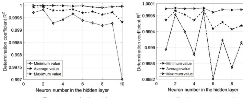
en-Figure 5.Influence of hidden-layer nodes onR2for different geoelectric models.
Figure 6.Distribution of resistivityρ1and thicknessh1in training samples.
gineering applications. It is the inversion input, and the out-puts are geoelectric structure parameters. A method which can avoid the complicated forward model calculation is of great importance in algorithm efficiency.
4.2 BP network design and the COPSO algorithm
For BP structure, the output nodes are determined by the number of inversion geoelectrical parameters, the input nodes are determined by the samples number ofHz(t ), and the hidden nodes vary according to approximation perfor-mance. As a three-layer or five-layer geoelectric model, its geoelectrical parameters are five (three resistivity and two thickness parameters) or nine (five resistivity and four thick-ness parameters); the output nodes are five or nine, corre-spondingly. The characteristic samplings ofHz(t )are chosen as 10 or 20, which are determined by the model’s complexity, with more layers meaning more sampling points needed. The 10 samplings were selected in this paper, hence with 10 input nodes. The hidden-layer neuron number is directly related to the weight and threshold parameter amount and greatly af-fects the BP performance. An appropriate hidden-node num-ber is necessary, and a determination coefficientR2is defined
for evaluation as
R2=
n
n
P
i=1
YiYˆi− n
P
i=1
Yi n
P
i=1
ˆ
Yi
2
n
n
P
i=1
ˆ
Yi2−
n P
i=1
ˆ
Yi
2! n
n
P
i=1
Yi2−
n P
i=1
Yi
2!, (20)
whereYi is the true value,Yˆi is the predicted value for the ith training data andnis the training data number. A larger determination coefficient means better approximation perfor-mance. The simulations on hidden-nodes effects were car-ried out for three-layer and five-layer geoelectric models. The BP structure is 10-s-5 and 10-s-9, and its transfer, training and learning functions are the “log sigmoidal”, “Levenberg– Marquardt” and “gradient descent momentum”, respectively. The average, minimum and maximum values ofR2were ob-tained after running 20 times for each simulation. The R2 curves were shown in Fig. 5.
Table 2.Comparison of different inertia weights in PSO algorithms (ωs=0.9 andωe=0.4).
Inertia Iteration Minimum Average Convergence
weight number fitness fitness time(s)
ω1 9 1.3914×10⁻³ 1.3982×10⁻³ 65.21
ω2 29 1.4406×10⁻³ 1.4418×10⁻³ 204.97
ω3 25 1.4168×10⁻³ 1.4224×10⁻³ 189.17
ωc 6 1.3846×10⁻³ 1.3925×10⁻³ 44.34
chosen as 10-2-5, and four types of inertia weight as in Eqs. (3)–(7) in the PSO were compared in Table 2.
The simulation was implemented on a Core (TM) i5-7500 processor with 8 GB of memory. It is obviously found in Ta-ble 2 that the COPSO algorithm has a much faster conver-gence rate and a lower iteration number and is time consum-ing.
4.3 Layered-model inversion
A three-layer and five-layer geoelectric models were inves-tigated, and the PSO parameter values are the same as those of the “Algorithm testing” section in this paper. In order to simulate actual TEM applications, the ramp turn-off is taken into account. Considering the probability distribution char-acteristic of the above algorithms, the average of 20 simula-tion results was chosen. The BP, SPSO-BP and COPSO-BP algorithms and a nonlinear programming genetic algorithm (NPGA) (Li et al., 2017) were compared.
4.3.1 Three-layer H-type model
The central loop TEM parameters were set as follows: the transmitting coil radius was set toa=100 m; the ramp emis-sion current was set to 100 A; and the turn-off time was set to 1 µs. In the geoelectric model, the resistivity isρ1=100, ρ2=10 andρ3=100m and the thickness ish1=100 and h2=200 m.
The BP training samples, which are a series of Hz(t ) for different geoelectrical parameters, were generated by the TEM forward model. The resistivity ranges were ρ1∈(50, 150),ρ2∈(5, 15) andρ3∈(50, 150) and the thickness ranges wereh1∈(50, 150) andh2∈(100, 300); 1000 random groups were chosen. The resistivity and thickness distributions ofρ1 andh1were shown in Fig. 6. The relative error is defined as
Err_rel=
T_cal∗ −O_ref∗ O_ref∗
, (21)
whereT_cal∗ andO_ref∗ are the calculated and reference values for the geoelectric models.
The inversion results were shown in Table 3 and Figs. 7– 8. The BP type algorithms were superior to the NPGA in-version in Table 3. Moreover, the inin-version accuracy,
conver-Figure 7.Fitness curves of SPSO-BP and COPSO-BP.
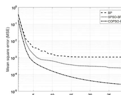
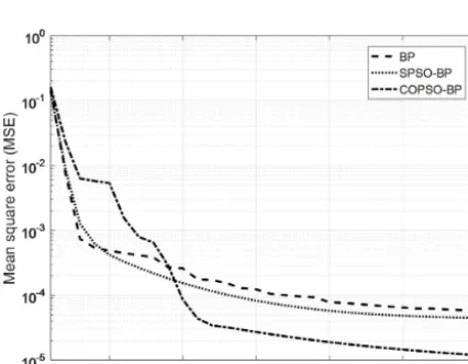
Figure 8.Comparison of mean square error curves.
gence rate and optimization ability of the COPSO-BP algo-rithm were better than others.
Additional results showed that the solution range of ρ1 andh1in the 20 simulations for the above algorithms were ρ1∈(97.980, 103.102) and h1∈(96.962, 102.480) for BP, ρ1∈(98.954, 101.137) andh1∈(96.955, 101.829) for SPSO-BP, ρ1∈(99.382, 100.989) and h1∈(97.877, 101.044) for COPSO-BP, respectively. Therefore, the COPSO-BP can ac-quire a higher accuracy and is more stable.
4.3.2 Five-layer KHK-type model
A five-layer KHK-type geoelectric model was adopted, and its resistivities wereρ1=100,ρ2=300,ρ3=50,ρ4=200 andρ5=30m, and its thickness wereh1=100,h2=200, h3=300 andh4=500 m.
Table 3.Inversion comparison of three-layer H-type geoelectric models.
H type Resistivityρ(m) Thicknessh(m) Total relative
ρ1 ρ2 ρ3 h1 h2 error (%)
True values 100 10 100 100 200 –
BP relative error (%) −0.275 −0.625 0.765 −0.968 −0.649 3.284 SPSO-BP relative error (%) 0.062 −0.322 −0.737 −0.579 −0.970 2.672
COPSO-BP 100.031 9.991 99.310 100.234 200.886 –
COPSO-BP relative error (%) 0.031 −0.087 −0.689 0.234 0.443 1.487 NPGA relative error (%) 0.133 −0.034 3.450 −7.305 −0.401 11.323
Figure 9.Fitness curves of SPSO-BP and COPSO-BP.
Figure 10.Comparison of mean square error curves.
1000 group training samples were generated within the above ranges. The inversion results were shown in Table 4 and Figs. 9–10. It can be seen that the COPSO-BP algorithm has better global optimization performance.
4.3.3 Inversion comparison
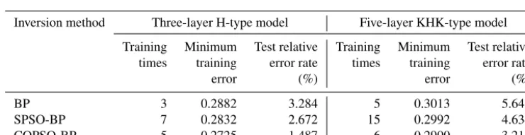
Three kinds of BP methods, the traditional BP, SPSO-BP and COPSO-BP algorithms, were compared in Table 5. Hence, the training times of COPSO-BP were obviously less than those of SPSO-BP and were almost equal to BP; it can obtain better precision especially for its global optimization perfor-mance.
The inversion of COPSO-BP and NPGA were compared in Fig. 11. The fitting ability of COPSO-BP was much better than NPGA.
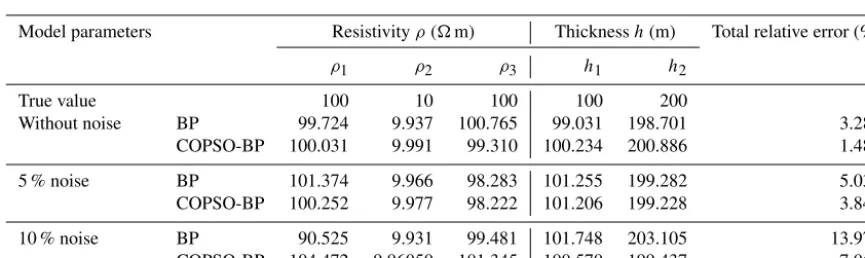
4.3.4 Robust performance analysis
In order to verify the algorithm robustness, 5 % (26 dB) and 10 % (20 dB) Gaussian random noise was added in TEM data for the three-layer geoelectric model. Three kinds of inver-sions were implemented respectively. The results and a com-parison were shown in Table 6. TheHz(t )and data with 5 % noise were shown in Fig. 12.
As can be seen in Table 2, after applying 5 % and 10 % Gaussian noise, the COPSO-BP inversion has a higher robust ability. The accuracy was obviously improved based on the total relative-error data.
4.4 Field example
resis-Table 4.Inversion comparison of five-layer KHK-type geoelectric models.
KHK type Resistivityρ(m) Thicknessh(m) Total relative
ρ1 ρ2 ρ3 ρ4 ρ5 h1 h2 h3 h4 error (%)
True values 100 300 50 200 30 100 200 300 500 –
BP relative error −1.006 −0.862 −1.014 −0.030 1.119 −0.362 −0.298 −0.575 −0.376 5.645 (%)
SPSO-BP relative 0.429 1.040 −0.577 −0.071 −0.883 −0.002 0.657 −0.655 −0.316 4.634 error (%)
COPSO-BP 99.594 299.469 50.082 199.092 29.937 99.501 200.481 301.800 497.670 –
COPSO-BP relative −0.405 −0.176 0.164 −0.453 −0.209 −0.498 0.240 0.600 −0.465 3.214 error (%)
NPGA relative −6.211 −0.008 −0.974 3.930 3.083 −0.691 0.505 −2.900 −3.370 19.062 error (%)
Table 5.Simulation comparison of different algorithms.
Inversion method Three-layer H-type model Five-layer KHK-type model
Training Minimum Test relative Training Minimum Test relative times training error rate times training error rate
error (%) error (%)
BP 3 0.2882 3.284 5 0.3013 5.645
SPSO-BP 7 0.2832 2.672 15 0.2992 4.634
COPSO-BP 5 0.2725 1.487 6 0.2900 3.214
tivity (300–400m), which is surmised to be the first-layer (T2g21) dolomite of the Middle Triassic old Malague sec-tion, with a thickness of about 400 m. The third layer has high resistivity (600–800m), which is speculated to be the sixth-layer (T2g16) limestone dolomite of the Middle Trias-sic old group. The results are baTrias-sically consistent with the geological conditions of the mining area, indicating the fea-sibility and effectiveness of the neural-network method. And the results of COPSO-BP inversion are better than those of the BP, for which the inversion position is more accurate, the shape and spacing are clearer, and the resistivity of each layer is more consistent with the those of the actual geologi-cal model.
5 Discussion
The inversion is performed for three-layer (H-type) and five-layer (KHK-type) geoelectric models in this paper. The re-sults show that the BP neural network is better than the NPGA algorithm because the BP method does not need to use the forward algorithm repeatedly, and its calculation time is short, which is different from the nonlinear heuristic method based on a global space search solution.
The main advantage of the BP is that it can interpret the transient electromagnetic sounding results quickly after training the network. Furthermore, the BP algorithm could automatically obtain the “reasonable rules” between input
and output data by learning, and it can adaptively store the learning content in the network weight, for which the BP neural network has a high self-learning and self-adaptation ability. In addition, the superior simulation results of the test function indicate that the BP algorithm can approximate any nonlinear continuous function with arbitrary precision, which means it has a strong nonlinear mapping ability; the inversion results of the layered geoelectric model with un-correlated noise data prove that the BP algorithm has strong robustness, which means it has the ability to apply learning results to new knowledge. However, the BP neural-network weight is gradually adjusted by the direction of local im-provement, which causes the algorithm to fall into a local extremum, and the weight converges to a local minimum that leads to the network training failure. Moreover, the BP is very sensitive to the initial network weight, and the initialization network with different weight values tends to converge at dif-ferent local minimums, so it obtains difdif-ferent results each time. In addition, the BP algorithm is essentially a gradient descent method, which leads to a slow convergence rate.
Figure 11.Inversion comparison of different geoelectric models.
Table 6.Comparison of inversion results of three-layer H-type (with noise) models.
Model parameters Resistivityρ(m) Thicknessh(m) Total relative error (%)
ρ1 ρ2 ρ3 h1 h2
True value 100 10 100 100 200 –
Without noise BP 99.724 9.937 100.765 99.031 198.701 3.284
COPSO-BP 100.031 9.991 99.310 100.234 200.886 1.487
5 % noise BP 101.374 9.966 98.283 101.255 199.282 5.039
COPSO-BP 100.252 9.977 98.222 101.206 199.228 3.847
10 % noise BP 90.525 9.931 99.481 101.748 203.105 13.976
COPSO-BP 104.472 9.96050 101.345 100.570 199.437 7.064
Figure 12.Forward data of Hz and data with 5 % noise.
and threshold of the BP neural network, which improves the global optimization performance of the algorithm. Further-more, the PSO algorithm adjusts the inertia weight adap-tively based on the chaotic-oscillation curve that is similar to the annealing process in the simulated annealing algo-rithm (SA), which jumps out the local extremum faster in the early stage and accelerates the convergence and reduces the training times. Therefore, compared with the SPSO-BP
and BP algorithms, the inversion results of COPSO-BP are closer to the theoretical data with smaller error fluctuations, stronger anti-noise controls, a better generalization of per-formance and higher stability, which it is effective in solving geophysical inverse problems.
From the simulation experiment, it is not clear how the weight organization affects the BP neural-network weight learning process. It is necessary to conduct a more system-atic study on this problem to improve our understanding of how the BP neural network handles training data.
6 Conclusions
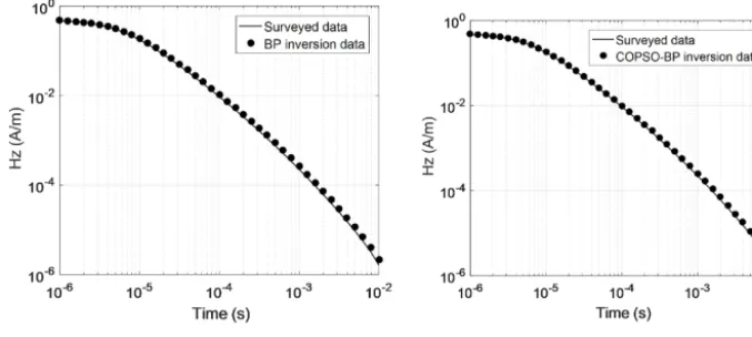
Figure 13.1-D inversion of forward results for(a)BP and(b)COPSO-BP.
Figure 14.Inversion results for BP(a)and COPSO-BP(b).
Code availability. The PSOBP code was developed by
Huaiqing Zhang and Ruiyou Li of Chongqing University in China, who are able to be contacted at the telephone number 13752954568 or e-mail address [email protected]. A computer with MATLAB R2016a is required is to run this code. The programming language of this code is C++, and its size is 10 KB. The source code is available at https://github.com/liruiyou/PSOBP (last access: 22 February 2019).
Author contributions. HZ conceived this paper. RL and HZ devel-oped the main algorithmic idea and the mathematical part. RL and NY carried out the simulation and data analysis. QZ completed the writing and interpretation of this paper. All authors contributed to the writing of the paper and approved the final paper.
Competing interests. The authors declare that they have no conflict of interest.
Acknowledgements. This work was partly supported by the Na-tional Natural Science Foundation of China (grant no. 51377174).
Financial support. This research has been supported by the Na-tional Natural Science Foundation of China (grant no. 51377174).
Review statement. This paper was edited by Norbert Marwan and reviewed by two anonymous referees.
References
Dai, Q., Jiang, F., and Dong, L.: Nonlinear inversion for electrical resistivity tomography based on chaotic DE-BP algorithm, J. Cent. South. Univ., 21, 2018–2025, https://doi.org/10.1007/s11771-014-2151-9, 2014.
Fernández Martínez, J. L., García Gonzalo, E., Fernández Álvarez, J. P., Kuzma, H. A., and Menéndez Pérez, C. O.: PSO: A pow-erful algorithm to solve geophysical inverse problems: Applica-tion to a 1D-DC resistivity case, J. Appl. Geophys., 71, 13–25, https://doi.org/10.1016/j.jappgeo.2010.02.001, 2010.
Jha, M. K., Kumar, S., and Chowdhury, A.: Vertical electri-cal sounding survey and resistivity inversion using genetic algorithm optimization technique, J. Hydrol., 359, 71–87, https://doi.org/10.1016/j.jhydrol.2008.06.018, 2008.
Jiang, F., Dai, Q., and Dong, L.: An ICPSO-RBFNN non-linear inversion for electrical resistivity imaging, J. Cent. South. Univ., 23, 2129–2138, https://doi.org/10.1007/s11771-016-3269-8, 2016a.
Jiang, F., Dai, Q., and Dong, L.: Nonlinear inversion of electri-cal resistivity imaging using pruning Bayesian neural networks, J. Appl. Geophys., 13, 267–278, https://doi.org/10.1007/s11770-016-0561-1, 2016b.
Jiang, F., Dong, L., and Dai, Q.: Electrical resistivity imaging in-version: An ISFLA trained kernel principal component wavelet neural network approach, Neural. Networks., 104, 114–123, https://doi.org/10.1016/j.neunet.2018.04.012, 2018.
Johnson, O. L. and Aizebeokhai, A. P.: Application of Artificial Neural Network for the Inversion of Electrical Resistivity Data, Journal of Informatics and Mathematical Sciences, 9, 297–316, 2017.
Kaufman, A. A. and Keller, G. V.: Frequency and Transient Sound-ing, Elsevier Methods in Geochemistry & Geophysics No 16, 620 pp., 1983.
Li, F. P., Yang, H. Y., and Liu, X. H.: Nonlinear programming ge-netic algorithm in transient electromagge-netic inversion, Geophys-ical and GeochemGeophys-ical Exploration, 41, 347–353, 2017.
Li, Y. Y., Chen, B. C., Zhao, Y. G., Yun, C., Ma, X. B., and Kong, X. R.: Nonlinear inversion for electrical resistivity tomography, Chi-nese J. Geophys., 52, 758–764, https://doi.org/10.1016/S1003-6326(09)60084-4, 2009.
Maiti, S., Erram, V. C., Gupta, G., and Tiwari, R. K.: ANN based inversion of DC resistivity data for groundwater exploration in hard rock terrain of western Maharashtra (India), J. Hydrol., 464, 294–308, https://doi.org/10.1016/j.jhydrol.2012.07.020, 2012. Pek¸sen, E., Yas, T., and Kıyak, A.: 1-D DC Resistivity
Mod-eling and Interpretation in Anisotropic Media Using Particle Swarm Optimization, Pure Appl. Geophys., 171, 2371–2389, https://doi.org/10.1007/s00024-014-0802-2, 2014.
Raj, A. S., Srinivas, Y., and Oliver, D. H.: A novel and generalized approach in the inversion of geoelectrical resistivity data using Artificial Neural Networks (ANN), J. Earth Syst. Sc., 123, 395– 411, https://doi.org/10.1007/s12040-014-0402-7, 2014. Rosas-Carbajal, M., Linde, N., Kalscheuer, T., and Vrugt, J. A.:
Two-dimensional probabilistic inversion of plane-wave electro-magnetic data: methodology, model constraints and joint inver-sion with electrical resistivity data, Geophys. J. Int., 196, 1508– 1524, https://doi.org/10.1093/gji/ggt482, 2014.
Sharma, S. P.: VFSARES – a very fast simulated annealing FOR-TRAN program for interpretation of 1-D DC resistivity sounding data from various electrode arrays, Comput. Geosci., 42, 177– 188, https://doi.org/10.1016/j.cageo.2011.08.029, 2012. Shi, F., Wang, X. C., and Yun, L.: Matlab neural network case study,
The Beijing University of Aeronautics & Astronautics Press, Beijing, 2010.
Shi, X. M., Xiao, M., Fan, J. K., Yang, G. S., and Zhang, X. H.: The damped PSO algorithm and its application for magnetotelluric sounding data inversion, Chinese J. Geophys., 52, 1114–1120, https://doi.org/10.3969/j.issn.0001-5733.2009.04.029, 2009. Srinivas, Y., Raj, A. S., Oliver, D. H., Muthuraj, D., and
Chan-drasekar, N.: A robust behavior of Feed Forward Back propa-gation algorithm of Artificial Neural Networks in the application of vertical electrical sounding data inversion, Geosci. Front., 3, 729–736, https://doi.org/10.1016/j.gsf.2012.02.003, 2012. Tran, K. T. and Hiltunen, D. R.: Two-Dimensional Inversion of Full
Waveforms Using Simulated Annealing, J. Geotech. Geoenviron. Eng., 138, 1075–1090, https://doi.org/10.1061/(ASCE)GT.1943-5606.0000685, 2012.
Wang, H., Liu M. L., Xi, Z. Z., Peng, X. L., and He, H.: Mag-netotelluric inversion based on BP neural network optimized by genetic algorithm, Chinese J. Geophys., 61, 1563–1575 https://doi.org/10.6038/cjg2018L0064, 2018.