https://doi.org/10.5194/amt-11-3177-2018 © Author(s) 2018. This work is distributed under the Creative Commons Attribution 4.0 License.
Neural network cloud top pressure and height for MODIS
Nina Håkansson1, Claudia Adok2, Anke Thoss1, Ronald Scheirer1, and Sara Hörnquist1
1Swedish Meteorological and Hydrological Institute (SMHI), Norrköping, Sweden 2Regional Cancer Center Western Sweden, Gothenburg, Sweden
Correspondence:Nina Håkansson ([email protected]) Received: 6 December 2017 – Discussion started: 30 January 2018 Revised: 20 April 2018 – Accepted: 3 May 2018 – Published: 1 June 2018
Abstract. Cloud top height retrieval from imager instru-ments is important for nowcasting and for satellite climate data records. A neural network approach for cloud top height retrieval from the imager instrument MODIS (Moderate Res-olution Imaging Spectroradiometer) is presented. The neural networks are trained using cloud top layer pressure data from the CALIOP (Cloud-Aerosol Lidar with Orthogonal Polar-ization) dataset.
Results are compared with two operational reference algo-rithms for cloud top height: the MODIS Collection 6 Level 2 height product and the cloud top temperature and height al-gorithm in the 2014 version of the NWC SAF (EUMETSAT (European Organization for the Exploitation of Meteorolog-ical Satellites) Satellite Application Facility on Support to Nowcasting and Very Short Range Forecasting) PPS (Polar Platform System). All three techniques are evaluated using both CALIOP and CPR (Cloud Profiling Radar for CloudSat (CLOUD SATellite)) height.
Instruments like AVHRR (Advanced Very High Resolu-tion Radiometer) and VIIRS (Visible Infrared Imaging Ra-diometer Suite) contain fewer channels useful for cloud top height retrievals than MODIS, therefore several different neural networks are investigated to test how infrared channel selection influences retrieval performance. Also a network with only channels available for the AVHRR1 instrument is trained and evaluated. To examine the contribution of dif-ferent variables, networks with fewer variables are trained. It is shown that variables containing imager information for neighboring pixels are very important.
The error distributions of the involved cloud top height al-gorithms are found to be non-Gaussian. Different descrip-tive statistic measures are presented and it is exemplified that bias and SD (standard deviation) can be misleading for non-Gaussian distributions. The median and mode are found to
better describe the tendency of the error distributions and IQR (interquartile range) and MAE (mean absolute error) are found to give the most useful information of the spread of the errors.
For all descriptive statistics presented MAE, IQR, RMSE (root mean square error), SD, mode, median, bias and per-centage of absolute errors above 0.25, 0.5, 1 and 2 km the neural network perform better than the reference algorithms both validated with CALIOP and CPR (CloudSat). The neu-ral networks using the brightness temperatures at 11 and 12 µm show at least 32 % (or 623 m) lower MAE compared to the two operational reference algorithms when validating with CALIOP height. Validation with CPR (CloudSat) height gives at least 25 % (or 430 m) reduction of MAE.
1 Introduction
and accurate cloud top height products from recent and past satellite measurements.
There are different traditional techniques to retrieve cloud top height see Hamann et al. (2014) for a presentation of 10 cloud top height retrieval algorithms applied to the SE-VIRI (Spinning Enhanced Visible Infrared Imager). Several algorithms to retrieve cloud top height from polar orbiting satellites are available and used operationally for nowcast-ing purposes or in cloud climatologies. These include the CTTH (cloud top temperature and height) from the PPS (Po-lar Platform System) package (Dybbroe et al., 2005), which is also used in the CLARA-A2 (Satellite Application Facil-ity for Climate Monitoring (CM SAF), cloud, albedo and surface radiation dataset from EUMETSAT (European Or-ganization for the Exploitation of Meteorological Satellites)) climate data record (Karlsson et al., 2017), ACHA (Algo-rithm Working Group (AWG) Cloud Height Algo(Algo-rithm) used in PATMOS-x (Pathfinder Atmospheres – Extended) (Hei-dinger et al., 2014), CC4CL (Community Cloud Retrieval for Climate) used in ESA (European Space Agency) Cloud_CCI (Cloud Climate Change Initiative) (Stengel et al., 2017), MODIS (Moderate Resolution Imaging Spectroradiometer) Collection-6 algorithm (Ackerman et al., 2015) and the IS-CCP (International Satellite Cloud Climatology Project) al-gorithm (Rossow and Schiffer, 1999).
We will use both the MODIS Collection-6 (MODIS-C6) and the 2014 version CTTH from PPS (PPS-v2014) as references to evaluate the performance of neural network based cloud top height retrieval. The MODIS-C6 algorithm is developed for the MODIS instrument. The PPS, deliv-ered by the NWC SAF (EUMETSAT Satellite Application Facility on Support to Nowcasting and Very Short Range Forecasting), is adapted to handle data from instruments such as AVHRR (Advanced Very High Resolution Radiome-ter), VIIRS (Visible Infrared Imaging Radiometer Suite) and MODIS.
Artificial neural networks are widely used for non-linear regression problems; see Gardner and Dorling (1998), Meng et al. (2007) or Milstein and Blackwell (2016) for exam-ples of neural network applications in atmospheric science. In CC4CL a neural network is used for the cloud detection (Stengel et al., 2017). Artificial neural networks have also been used on MODIS data to retrieve cloud optical depth (Minnis et al., 2016). The COCS (cirrus optical properties; derived from CALIOP and SEVIRI) algorithm uses artifi-cial neural networks to retrieve cirrus cloud optical thickness and cloud top height for the SEVIRI instrument (Kox et al., 2014). Considering that neural networks in the mentioned ex-amples have successfully derived cloud properties, and that cloud top height retrievals often include fitting of brightness temperatures to temperature profiles, a neural network can be expected to retrieve cloud top pressure for MODIS with some skill.
One type of neural network is the multilayer perceptron described in (Gardner and Dorling, 1998) which is a
super-vised learning technique. If the output for a certain input, when training the multilayer perceptron, is not equal to the target output an error signal is propagated back in the net-work and the weights of the netnet-work are adjusted resulting in a reduced overall error. This algorithm is called the back-propagation algorithm.
In this study we will compare the performance of back-propagation neural network algorithms for retrieving cloud top height (NN-CTTH) with the CTTH algorithm from PPS version 2014 (PPS-v2014) and MODIS Collection 6 (MODIS-C6) algorithm. Several networks will be trained to estimate the contribution of different training variables to the overall result. The networks will be validated using both CALIOP (Cloud-Aerosol Lidar with Orthogonal Polariza-tion) and CPR (Cloud Profiling Radar for CloudSat (CLOUD SATellite)) height data.
In Sect. 2 the different datasets used are briefly described and in Sect. 3 the three algorithms are described. Results are presented and discussed in Sect. 4 and final conclusions are found in Sect. 5.
2 Instruments and data
For this study we used data from the MODIS instrument on the polar orbiting satellite Aqua in the A-Train, as it is co-located with both CALIPSO (Cloud-Aerosol Lidar and Infrared Pathfinder Satellite Observations) and CloudSat at most latitudes and has multiple channels useful for cloud top height retrieval.
2.1 Aqua – MODIS
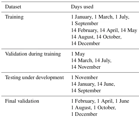
The MODIS is a spectroradiometer with 36 channels cover-ing the solar and thermal spectra. We are uscover-ing level 1 data from the MODIS instrument on the polar orbiter Aqua. For this study the MYD021km (MODIS Science Data Support Team, 2015a) and MYD03 (MODIS Science Data Support Team, 2015b) for all orbits from 24 dates were used (the 1st and 14th of every month of 2010). The data were divided into four parts which were used for training, validation dur-ing traindur-ing (used to decide when to quit traindur-ing), testdur-ing un-der development (used to test different combinations of vari-ables during prototyping) and final validation. The data con-tains many pixels that are almost identical, because a typical cloud is larger than one pixel. Therefore randomly dividing the data into four datasets is not possible as this would, in practice, give four identical datasets which would cause the network to over-train. See Table 1 for distribution of data.
Table 1.MODIS data from 2010 used for training and validation of the neural networks.
Dataset Days used
Training 1 January, 1 March, 1 July, 1 September
14 February, 14 April, 14 May 14 August, 14 October, 14 December
Validation during training 1 May
14 March, 14 July, 14 November
Testing under development 1 November 14 January, 14 June, 14 September
Final validation 1 February, 1 April, 1 June 1 August, 1 October, 1 December
The satellite zenith angles for MODIS when matched with CALIOP vary between 0.04 and 19.08◦; when matched with CPR (CloudSat) they vary between 0.04 and 19.26◦. 2.2 CALIOP
The CALIOP lidar on the polar orbiting satellite CALIPSO is an active sensor and therefore more sensitive to particle con-glomerates with low density than typical imagers. The hori-zontal pixel resolution is 0.07 km×0.333 km, this means that when co-locating with MODIS one should remember that CALIOP samples only a small part of each MODIS pixel. The vertical resolution for CALIOP is 30 m. The viewing an-gle for CALIOP is 3◦. The CALIOP 1 km Cloud Layer prod-uct data were used (for the dates, see Table 1) as the truth to train the networks against, and for validation of the net-works. The 1 km product was selected because the resolution is closest to the MODIS resolution. For training version 3 of the CALIOP data was used. The final validation was made with version 4 because of the more accurate cloud type in-formation in the feature classification flag in version 4. 2.3 CPR (CloudSat)
The CPR (CloudSat) is a radar which derives a ver-tical profile of cloud water. Its horizontal resolution is 1.4 km×3.5 km, its vertical resolution is 0.5 km and the viewing angle is 0.16◦. The CPR (CloudSat) product 2B-GEOPROF-R05 (Marchand et al., 2008) was used as an addi-tional source for independent validation of the networks, see Table 1 for selected dates. The validation with CPR (Cloud-Sat) will have a lower percentage of low clouds compared to CALIOP because ground clutter is a problem for space-borne radar instruments.
2.4 Other data
Numerical weather prediction (NWP) data are needed as in-put for the PPS-v2014 and the neural network algorithm. In this study the operational 91-level short-range archived forecasted NWP data from ECMWF (European Centre for Medium-range Weather Forecasting) were used. The anal-ysis times 00:00 and 12:00 were used in combination with the following forecast times: 6, 9, 12 and 15 h. Under the period Integrated Forecast System (IFS) cycles 35r3, 36r1, 36r3 and 36r4 were operational. Ice maps (OSI-409 version 1.1) from OSISAF (Satellite Application Facility on Ocean and Sea Ice) were also used as input for the PPS cloud mask algorithm.
3 Algorithms
3.1 PPS-v2014 cloud top temperature and height
The cloud top height algorithm in PPS-v2014, uses two dif-ferent algorithms for cloud top height retrieval, one for pixels classified as opaque and another for semitransparent clouds. The reason for having two different algorithms is that the straight forward opaque algorithm can not be used for pix-els with optically thin clouds like cirrus or broken cloud fields like cumulus. The signals for these pixels are a mixture of contributions from the cloud itself and underlying clouds and/or the surface.
The algorithm uses a split-window technique to decide whether to apply the opaque or semitransparent retrieval. All pixels with a difference between the 11 and 12 µm brightness temperatures of more than 1.0 K are treated as semitranspar-ent. This is a slight modification of the PPS version 2014 al-gorithm where the clouds classified as non-opaque by cloud type product are also considered semitransparent.
The retrieval for opaque clouds matches the observed brightness temperatures at 11 µm against a temperature pro-file derived from a short term forecast or (re)analysis of a NWP model, adjusted for atmospheric absorption. The first match, going along the profile from the ground and upwards, gives the cloud top height and pressure. Temperatures colder or warmer than the profile are fitted to the coldest or warmest temperature of the profile below tropopause, respectively.
for opaque clouds. For more detail about the algorithms see SMHI (2015).
PPS height uses the unit altitude above ground. For all comparisons this is transformed to height above mean sea level, using elevations given in the CPR (CloudSat) or CALIOP datasets.
3.2 MODIS Collection 6 Aqua Cloud Top Properties product
In MODIS Collection 6 the CO2slicing method (described
in Menzel et al., 2008) is used to retrieve cloud top pressure using the 13 and 14 µm channels for ice clouds (as deter-mined from MODIS phase algorithm). For low level clouds the 11 µm channel and the IR-window approach (IRW) with a latitude dependent lapse rate is used over ocean (Baum et al., 2012). Over land the 11 µm temperature is fitted against an 11 µm temperature profile calculated from GDAS (Global Data Assimilation System) temperature, water vapor and ozone profiles and the PFAAST (Pressure-Layer Fast Al-gorithm for Atmospheric Transmittance) radiative transfer model is used for low clouds (Menzel et al., 2008). For more details about the updates in Collection 6 see Baum et al. (2012). Cloud pressure is converted to temperature and height using the National Centers for Environmental Predic-tion Global Data AssimilaPredic-tion System (Baum et al., 2012). 3.3 Neural network cloud top temperature and height
NN-CTTH
Neural networks are trained using MODIS data co-located with CALIOP data. Nearest neighbor matching was used with the pyresample package in the PyTroll project (Raspaud et al., 2018). The Aqua and CALIPSO satellites are both part of the A-Train and the matched FOV (field of view) are close in time (only 75 s apart). The uppermost top layer pres-sure variable, for both multi- and single-layer clouds, from CALIOP data was used as training truth. Temperature and height for the retrieved cloud top pressure are extracted us-ing NWP data. Pressure predicted higher than surface pres-sure are set to surface prespres-sure. For prespres-sures lower than 70 hPa neither height nor temperature values are extracted. The amount of pixels with pressure lower than 70 hPa varies between 0 and 0.05 % for the networks.
3.3.1 Neural network variables
To reduce sun zenith angle dependence and to have the same algorithm for all illumination conditions only infrared chan-nels were used to train the neural networks. Several different types of variables were consequently used to train the net-work; the most basic variables were the NWP temperatures at the following pressure levels: surface, 950, 850, 700, 500 and 250 hPa. This together with the 11 or 12 µm brightness temperature (B11orB12) gave the network what was needed
to make a radiance fitting to retrieve cloud top pressure for
opaque clouds, although with very coarse vertical resolution in the NWP data. For opaque clouds that are geometrically thin, with little or no water vapor above the cloud, the 11 and 12 µm brightness temperatures will be the same as the cloud top temperature. If the predicted NWP temperatures are correct the neural network could fit the 11 µm brightness temperature to the NWP temperatures and retrieve the cloud pressure (similar to what is done in PPS-v2014 and MODIS-C6). For cases without inversions in the temperature profile, the retrieved cloud top pressure should be accurate. The cases with inversions are more difficult to fit correctly, as multiple solutions exist and the temperature inversion might not be accurately captured with regards to its strength and height in the NWP data. For semitransparent clouds the network needs more variables to make a correct retrieval.
To give the network information on the opacity of the pixel, brightness temperature difference variables were in-cluded (B11−B12,B11−B3.7,B8.5−B11). Texture variables
with the standard deviation of brightness temperature, or brightness temperature difference, for 5×5 pixels were in-cluded. These contain information about whether pixels with largeB11−B12are more likely to be semitransparent or more
likely to be fractional or cloud edges.
As described in Sect. 3.1, PPS-v2014 usesB11−B12 and B11 of the neighboring pixels to retrieve temperatures for
semitransparent clouds. In order to feed the network with some of this information the neighboring warmest and cold-est pixels inB11 in a 5×5 pixel neighborhood were
iden-tified. Variables using the brightness temperature at these warmest and coldest pixels were calculated, for example the 12 µm brightness temperature for the coldest pixel minus the same for the current pixel:B12C−B12, see Table 2 for more
information about what variables were calculated.
The surface pressure was also included, which provides the network with a value for the maximum reasonable pres-sure. Also the brightness temperature for the CO2channel at
13.3 µm and the water vapor channels at 6.7 and 7.3 µm were included as variables. The CO2channel at 13.3 µm is used in
the CO2slicing method of MODIS-C6 and should improve
the cloud top height retrieval for high clouds.
The instruments AVHRR, VIIRS, MERSI-2 (Medium Resolution Spectral Imager-2), MetImage (Meteorological Imager) and MODIS all have different selections of IR chan-nels; however most of them have the 11 and 12 µm channels. The first AVHRR instrument, AVHRR1, only had two IR channels at 11 and 3.7 µm and no channel at 12 µm. Networks were trained using combinations of MODIS IR-channels cor-responding to the channels available for the other instru-ments. See Table 3 for specifications of the networks trained. Table 4 gives an overview of what imager channels were used for which network.
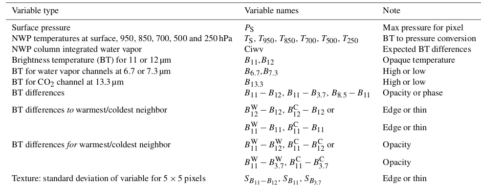
Table 2.Description of variable types used to train the neural networks.
Variable type Variable names Note
Surface pressure PS Max pressure for pixel
NWP temperatures at surface, 950, 850, 700, 500 and 250 hPa TS,T950,T850,T700,T500,T250 BT to pressure conversion
NWP column integrated water vapor Ciwv Expected BT differences
Brightness temperature (BT) for 11 or 12 µm B11,B12 Opaque temperature
BT for water vapor channels at 6.7 or 7.3 µm B6.7,B7.3 High or low
BT for CO2channel at 13.3 µm B13.3 High or low
BT differences B11−B12,B11−B3.7,B8.5−B11 Opacity or phase
BT differencestowarmest/coldest neighbor B12W−B12,B12C−B12or Edge or thin B11W−B11,B11C−B11 Edge or thin
BT differencesforwarmest/coldest neighbor B11W−B12W,B11C −B12C or Opacity B11W−B3.7W,B11C−B3.7C Opacity Texture: standard deviation of variable for 5×5 pixels SB11−B12,SB11,SB3.7 Edge or thin
Table 3.Description of the different networks. See Table 2 for explanation of the variables. The NWP variables:PS,TS,T950,T850,T700, T500,T250are used in all networks.
Network name Network specific variables
NN-NWP Ciwv
NN-OPAQUE B12
NN-BASIC B12,B11−B12,
NN-BASIC-CIWV B12,B11−B12, Ciwv
NN-AVHRR B12,B11−B12, Ciwv,B11W−B12W,B11C−B12C,B12W−B12,B12C−B12,SB11−B12,SB11
NN-VIIRS B12,B11−B12, Ciwv,B11W−B12W,B11C−B12C,B12W−B12,B12C−B12,SB11−B12,SB11,B8.5−B11 NN-MERSI-2 B12,B11−B12, Ciwv,B11W−B12W,B11C−B12C,B12W−B12,B12C−B12,SB11−B12,SB11,B8.5−B11,B7.3 NN-MetImage-NoCO2 B12,B11−B12, Ciwv,B11W−B12W,B11C−B12C,B12W−B12,B12C−B12,SB11−B12,SB11,B8.5−B11,B7.3,
B6.7
NN-MetImage B12,B11−B12, Ciwv,B11W−B12W,B11C−B12C,B12W−B12,B12C−B12,SB11−B12,SB11,B8.5−B11,B7.3, B6.7,B13.3
NN-AVHRR1 B11,B11−B3.7, Ciwv,B11W−B3.7W,B11C−B3.7C ,B11W−B11,B11C−B11,SB3.7,SB11
check. For this network we expect bad results. However good results for this network would indicate that height informa-tion retrieved was already available in the NWP data.
3.3.2 Training
For the training 1.5 million pixels were used, with the distri-bution 50 % low clouds, 25 % medium level clouds and 25 % high clouds. A higher percentage of low clouds was included because the mean square error (MSE) is often much higher for high clouds. Previous tests showed that fewer low clouds caused the network to focus too much on predicting the high clouds correctly and showed degraded results for low clouds. For the validation dataset used during training 375 000
pix-els were randomly selected with the same low/medium/high distribution as for the training data.
The machine learning module scikit-learn (Pedregosa et al., 2011), the Keras package (Keras Team, 2015), the Theano backend (Theano Development Team, 2016) and the Python programming language were used for training the network.
3.3.3 Parameters and configurations
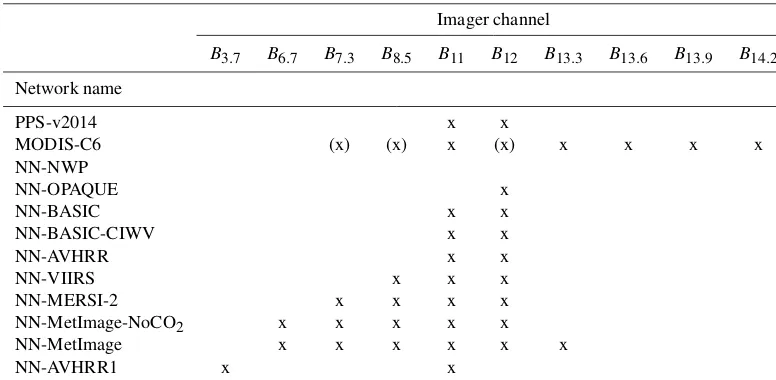
Table 4.Description of the imager channels used for the different algorithms. For MODIS-C6 channels used indirectly, to determine if CO2-slicing should be applied, are noted with brackets.
Imager channel
B3.7 B6.7 B7.3 B8.5 B11 B12 B13.3 B13.6 B13.9 B14.2
Network name
PPS-v2014 x x
MODIS-C6 (x) (x) x (x) x x x x
NN-NWP
NN-OPAQUE x
NN-BASIC x x
NN-BASIC-CIWV x x
NN-AVHRR x x
NN-VIIRS x x x
NN-MERSI-2 x x x x
NN-MetImage-NoCO2 x x x x x
NN-MetImage x x x x x x
NN-AVHRR1 x x
Choosing the number of hidden neurons and hidden layers of the neural network is also important for the training to be effective. Too few hidden neurons will result in under-fitting. We used two hidden layers with 30 neurons in the first layer and 15 neurons in the second.
The initialization of weights before training the network is important for the neural network to learn faster. There are many different weight initialization methods for training the networks; however in this case the Glorot uniform weight ini-tialization was used. The activation function used for the hid-den layers was the tangent hyperbolic (see Karlik and Olgac, 2011) and for the output layer a linear activation function was used.
To determine the changes in the weights an optimization method was used during the back-propagation algorithm. The optimization method used for the multilayer perceptron is mini-batch stochastic gradient descent which performs mini-batch training. A mini-batch is a sample of observations in the data. Several observations are used to update weights and biases, which is different from the traditional stochas-tic gradient descent where one observation at a time is used for the updates (Cotter et al., 2011). Having an optimal mini-batch size is important for the training of a neural network because overly large batches can cause the network to take a long time to converge; we used a mini-batch size of 250.
When training the neural network there are different learn-ing parameters that need to be tuned to ensure an effec-tive training procedure. During prototyping several different combinations were tested. The learning rate is a parameter that determines the size of change in the weights. On one hand, a learning rate that is too high will result in large weight changes and can result in an unstable model (Hu and Weng, 2009). On the other hand, if a learning rate is too low the
training time of the network will be long; we used a learning rate of 0.01.
The momentum is a parameter which adds a part of the weight change to the current weight change, using momen-tum can help avoid the network getting trapped in local min-ima (Gardner and Dorling, 1998). A high value of tum speeds up the training of the network; we had a momen-tum of 0.9. The parameterlearning rate decay, set to 10−6, in Keras, is used to decrease the learning rate after each update as the training progresses.
To avoid the neural network from over-fitting (which makes the network extra sensitive to unseen data), a method calledearly stoppingwas used. In early stopping the valida-tion error is monitored during training to prevent the network from over-fitting. If the validation error is not improved for some (we used 10) epochs training is stopped. The network for which the validation error was at its lowest is then used. The neural networks were trained for a maximum of 2650 epochs, but the early stopping method caused the training to stop much earlier.
4 Results and discussion
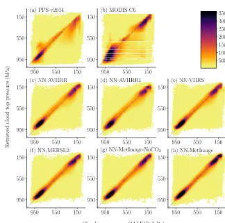
Figure 1.Scatter plots of the pressure for the neural networks and for the reference methods against CALIOP cloud top pressure. The data were divided in 10×10 (hPa) bins for color coding. The number of points in each bin determines the color of the point. The final validation dataset (see Table 1) where all algorithms had a height reported is used.
used for CPR (CloudSat) to include only strong detections. The coarser vertical resolution for CPR (CloudSat) of 500 m means that MAE is expected to be higher than 250 m com-pared to 15 m for CALIOP.
The scatter plots in Fig. 1 show how the cloud top pres-sure retrievals of the neural networks and the reference meth-ods are distributed compared to CALIOP. Figure 2 show the same type of scatter plots for cloud top height with CPR (CloudSat) as truth. These scatter plots show that all neu-ral networks have similar appearance with most of the data retrieved close to the truth. All methods (NN-CTTH, PPS-v2014 and MODIS-C6) retrieve some heights and pressures that are very far from the true values of CPR (CloudSat) or CALIOP. It is important to remember that some of these seemingly bad results are due to the different FOVs for the MODIS and the CALIOP or CPR (CloudSat) sensors.
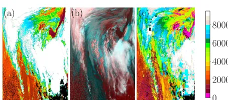
Figure 3 compares the NN-AVHRR and PPS-v2014 for one scene. For semitransparent clouds PPS-v2014 retrieves the same result for 32×32 pixels, which can be seen as blue squares in Fig. 3c. We also observe that a lot of high clouds are placed higher by NN-AVHRR (pixels that are blue in panel (c)and white in panel(a)). For NN-AVHRR
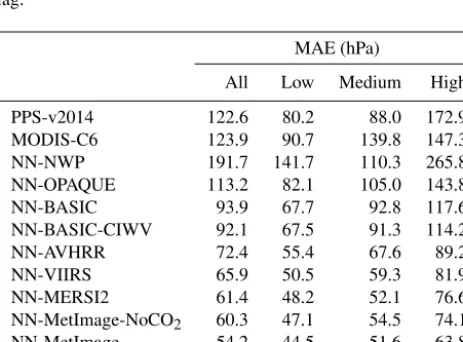
in panel(a)we can see that the large area with low clouds in the lower left corner gets a consistent cloud top height (the same orange color everywhere). Note that the NN-AVHRR has a less noisy appearance and has less “missing data”. 4.1 Validation with CALIOP top layer pressure First we consider the performance of all the trained networks validated with the uppermost CALIOP top layer pressure in terms of mean absolute error (MAE). Results in Table 5 show that both PPS-v2014 and MODIS-C6 have a MAE close to 120 hPa. Notice that the network using only the NWP in-formation and no imager channels (NN-NWP) shows high MAE. This was included as a sanity check to see that the neural networks are mainly using the satellite data, and the high MAE for NN-NWP supports this. The NN-OPAQUE network using onlyB12and the basic NWP data has a 9 hPa
improvement in MAE compared to the reference algorithms. By including the variableB11−B12, the MAE improves by
an additional 19 hPa becauseB11−B12contains information
Figure 2.Scatters plot of the height for the neural networks and for the reference methods against CPR (CloudSat) height. The data were divided in 0.25×0.25 (km) bins for color coding. The number of points in each bin determines the color of the point. The final validation dataset (see Table 1) where all algorithms had a height reported is used. Two points where CPR (CloudSat) had a height above 22 km where excluded. A cloudy threshold of 30 % is used for CPR (CloudSat).
Figure 3.Comparing the cloud top height from the NN-AVHRR(a)
to PPS-v2014(c)with a RGB in the middle(b)using channels at 3.7, 11 and 12 µm. Notice that the NN-AVHRR is smoother, con-tains less“missing data (black)” and that the small high ice clouds in the lower part of the figure are better captured. This is from MODIS on Aqua 14 January 2010, 00:05 UTC.
of 2 hPa on MAE. However adding all variables containing information on neighboring pixels improves the result by an additional 20 hPa. The NN-AVHRR network using 11 and 12 µm from MODIS provides an MAE which is reduced by
about 50 hPa compared to both from MODIS-C6 and PPS-v2014. Notice also that the scores improve for all categories (low, medium and high) when compared with both PPS-v2014 and MODIS-C6. The inclusion of the neighboring pix-els accounts for almost 40 % of the improvement. Note that for medium level clouds NN-BASIC-CIWV, without infor-mation from neighboring pixels, has higher MAE compared to PPS-v2014.
Adding more IR channels further improves the results. Adding channel 8.5 µm (B8.5−B11, NN-VIIRS) improves
MAE by 7 hPa and adding 7.3 µm (B7.3, NN-MERSI-2)
im-proves MAE by 5 hPa. Including the other water vapor chan-nel at 6.7 µm (B6.7, NN-MetImage-NoCO2) only improves
MAE by 1 hPa. The CO2 channel at 13.3 µm (B13.3,
NN-MetImage) improves the MAE by an additional 6 hPa. The NN-AVHRR1 network trained using 3.7 and 11 µm (MAE 76.1 hPa) is a little worse than NN-AVHRR (MAE 72.4 hPa). Note thatB3.7has a solar component which is currently not
treated in any way. IfB3.7was corrected for the solar
Figure 4.Retrieved pressure dependence on satellite zenith angle. CALIOP pressure distribution is shown in light blue. The percent of cloud top pressure results are calculated in 50 hPa bins. The final validation dataset is used (see Table 1).
Table 5.Mean absolute error (MAE) for different algorithms com-pared to CALIOP top layer pressure. The final validation dataset (see Table 1), containing 1 832 432 pixels (45 % high, 39 % low and 16 % medium level clouds) is used. Pixels with valid pressure for PPS-v2014, MODIS-C6, and CALIOP are considered. The low, medium and high classes are from CALIOP feature classification flag.
MAE (hPa)
All Low Medium High
PPS-v2014 122.6 80.2 88.0 172.9
MODIS-C6 123.9 90.7 139.8 147.3
NN-NWP 191.7 141.7 110.3 265.8
NN-OPAQUE 113.2 82.1 105.0 143.8
NN-BASIC 93.9 67.7 92.8 117.6
NN-BASIC-CIWV 92.1 67.5 91.3 114.2
NN-AVHRR 72.4 55.4 67.6 89.2
NN-VIIRS 65.9 50.5 59.3 81.9
NN-MERSI2 61.4 48.2 52.1 76.6
NN-MetImage-NoCO2 60.3 47.1 54.5 74.1
NN-MetImage 54.2 44.5 51.6 63.8
NN-AVHRR1 76.1 54.7 69.9 97.3
scores for all categories (low, medium, and high) compared to PPS-v2014 and MODIS-C6.
The training with CALIOP using only MODIS from Aqua includes only near NADIR observations with all satellite zenith angles for MODIS below 20◦. Figure 4 shows that NN-AVHRR and NN-AVHRR1 networks also perform ro-bustly also for higher satellite zenith angles. The NN-VIIRS and NN-MetImage-NoCO2results deviate for satellite zenith
angles larger than 60◦. The NN-MERSI-2 results deviate for satellite zenith angles larger than 40◦. The NN-MetImage re-trieval already shows deviations above 20◦ satellite zenith angle and for satellite zenith angles larger than 40 the re-trieval has no predictive skill. Notice that the distribution for MODIS-C6 also depends on the satellite zenith angle (with fewer high clouds at higher angles). For PPS-v2014, in com-parison, fewer low clouds are found at higher satellite zenith angles. The neural networks (NN-AVHRR, NN-AVHRR1, NN-VIIRS and NN-MetImage-NoCO2) can reproduce the
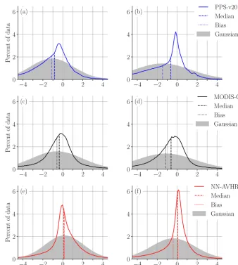
Figure 5.Error distribution compared to CPR (CloudSat)(a, c, e)and CALIOP(b, d, f)with biases and medians marked. The percent of data is calculated in 0.1 km bins. The final validation dataset (see Table 1) where all algorithms had a height reported is used. Note that the values on theyaxis are dependent on the bin size. The peak at 6 % for NN-AVHRR in(f), means that 6 % of the retrieved heights are between the CALIOP height and the CALIOP height+0.1 km. The Gaussian distribution with the same bias and standard derivation is shown in grey.
4.2 Discussion of statistics measures for non-Gaussian error distributions
For pressure we choose a single measure, MAE, to describe the error; however which (and how many) measures are needed to adequately describe the error distribution need to be discussed. For a Gaussian error distribution the obvious choices are bias and SD (standard deviation) as the Gaussian error distribution is completely determined from bias and SD and all other important measures could be derived from bias and SD. Unfortunately the error distributions considered here are non-Gaussian. This is expected, as we know that apart from the errors of the algorithm and the errors due to differ-ent FOV we expect the lidar to detect some thin cloud layers not visible to the imager. These thin layers, not detected by the imager, should result in underestimated cloud top heights.
In Fig. 5 the error distributions for MODIS-C6, PPS-v2014 and NN-AVHRR are shown. The Gaussian error distribution with the same bias and SD are plotted in grey. It is clear that the bias is not at the center (the peak) of the distribution. The median is not at the center either, but closer to it. For vali-dation with CALIOP we can see the expected negative bias for all algorithms and for all cases we can also observe that assuming a Gaussian distribution underestimates the amount of small errors.
PEx=
number of absolute errors> xkm
number of errors (1)
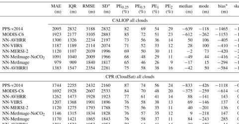
Table 6.Statistic measures for the error distributions for all clouds. For all measures except skewness it is the case that values closer to zero are better. The statistics are calculated for 1 198 599 matches for CPR (CloudSat) and 1 803 335 matches for CALIOP. A small amount 0.2 % of the matches were excluded because of missing height or pressure below 70 hPa for any of the algorithms. PEXdescribes percentage of
absolute errors aboveXkm, see Eq. (1).
MAE IQR RMSE SD∗ PE0.25 PE0.5 PE1 PE2 median mode bias∗ skew
(m) (m) (m) (m) (%) (%) (%) (%) (m) (m) (m)
CALIOP all clouds
PPS-v2014 2095 2832 3188 2832 82 69 54 29 −639 −118 −1465 −1.0
MODIS-C6 1923 2177 3105 2883 85 72 51 23 −612 −262 −1153 −1.5
NN-AVHRR 1300 1326 2234 2197 73 56 36 14 50 106 −405 −1.8
NN-VIIRS 1187 1189 2114 2074 71 52 33 12 28 100 −410 −1.9
NN-MERSI-2 1120 1107 2039 1996 69 50 30 11 −2 73 −420 −2.0
NN-MetImage-NoCO2 1091 1040 2009 1966 68 48 29 11 −49 44 −416 −2.0
NN-MetImage 979 909 1840 1817 65 46 26 9 −17 15 −294 −1.9
NN-AVHRR1 1383 1547 2354 2281 75 58 38 16 −42 50 −584 −1.8
CPR (CloudSat) all clouds
PPS-v2014 1744 2255 2432 2160 87 74 56 24 −833 −426 −1118 −0.1
MODIS-C6 1692 1928 2607 2533 84 70 48 20 −375 −259 −614 −0.1
NN-AVHRR 1262 1473 1928 1923 77 61 41 14 88 −141 143 0.2
NN-VIIRS 1207 1368 1901 1896 76 58 38 13 69 −146 137 0.5
NN-MERSI-2 1120 1275 1793 1788 75 56 35 11 40 −201 136 0.5
NN-MetImage-NoCO2 1146 1315 1834 1828 76 57 35 12 9 −218 147 0.7
NN-MetImage 1170 1421 1865 1843 76 58 37 11 84 −243 285 0.9
NN-AVHRR1 1281 1523 1953 1953 79 63 41 14 30 −128 −14 0.0
∗Interpret bias and SD with caution as distributions are non-Gaussian. Bias is not located at the center of the distribution.
distributions are skewed and non-Gaussian. The mode is cal-culated using the half-range method to robustly estimate the mode from the sample (for more info see Bickel, 2002). The bias should be interpreted with caution. Consider PPS-v2014 compared to CALIOP (Table 6), if we add 1465 to all re-trievals creating a “corrected” retrieval we would have an er-ror distribution with the same SD and zero bias but the cen-ter (peak) of the distribution would not be closer zero. The PE1(percentage of absolute errors above 1 km, see Eq. 1) for
this “corrected” retrieval would increase from 54 to 73 %! For the user this is clearly not an improvement. The general over estimation of cloud top heights of this “corrected” re-trieval would, however, be detected by the median and the mode which would be further away from zero but now on the positive side. This example illustrates the risk of misinterpre-tation of the bias for non-Gaussian error distributions.
Several different measures of variation are presented in Ta-ble 6 MAE, IQR (interquartile range), SD and RMSE. The measures have different benefits; IQR are robust against out-liers and RMSE and SD focus on the worst retrievals as errors are squared. Considering that it is likely not interesting if use-less retrievals with large errors are 10 km off or 15 km off, in combination with the fact that some large errors are expected due to different FOV and different instrument sensitivities, the MAE and IQR provide more interesting measures of vari-ation compared to the SD and the RMSE. In the example
dis-cussed in the previous section the MAE for the “corrected” retrieval would change only 10 m but the RMSE (root mean square error) would improve estimations by 356 m indicat-ing a much better algorithm; when in fact it is a degraded algorithm. If the largest errors are considered very important RMSE is preferred over SD for skewed distributions, espe-cially if bias is also presented. This is owing to the fact that RMSE and bias have a smaller risk of being misinterpreted by the reader as a Gaussian error distribution.
For low level clouds we have even stronger reasons to ex-pect skewed distributions as there is always a limit (ground) to how low clouds top heights can be underestimated and Ta-ble 7 shows that the skewness is large for low level clouds. The bias for low level clouds is difficult to interpret as it is the combination of the main part of the error distribution lo-cated close to zero and the large positive errors (which are to some extent expected due to different FOVs). In Fig. 6e and f the error distributions for MODIS-C6, PPS-v2014 and NN-AVHRR for low level clouds are shown. We can see, in Fig. 6, that the NN-AVHRR less often underestimates the cloud top height for low level clouds which partly explains the higher bias for NN-AVHRR.
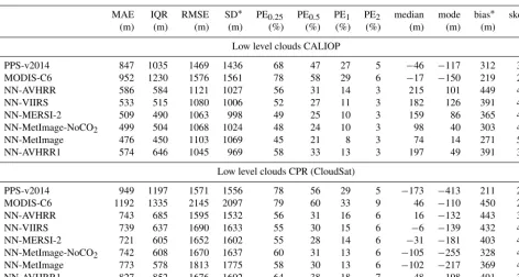
Un-Table 7.Statistic measures for the error distributions for low level clouds. For all measures except skewness it is the case that values closer to zero are better. The statistics are calculated for 328 015 matches for CPR (CloudSat) and 709 434 matches for CALIOP. The low class comes from CALIOP feature classification flag (class 0, 1, 2 and 3) and for CPR (CloudSat) it is the pixels with heights lower or exactly at the NWP height at 680 hPa. PEXdescribes percentage of absolute errors aboveXkm, see Eq. (1).
MAE IQR RMSE SD∗ PE0.25 PE0.5 PE1 PE2 median mode bias∗ skew
(m) (m) (m) (m) (%) (%) (%) (%) (m) (m) (m)
Low level clouds CALIOP
PPS-v2014 847 1035 1469 1436 68 47 27 5 −46 −117 312 3.0
MODIS-C6 952 1230 1576 1561 78 58 29 6 −17 −150 219 2.9
NN-AVHRR 586 584 1121 1027 56 31 14 3 215 101 449 4.0
NN-VIIRS 533 515 1080 1006 52 27 11 3 182 126 391 4.8
NN-MERSI-2 509 490 1063 998 49 25 10 3 159 86 365 4.8
NN-MetImage-NoCO2 499 504 1068 1024 48 24 10 3 98 40 303 4.9
NN-MetImage 476 450 1103 1069 45 21 8 3 74 14 271 5.4
NN-AVHRR1 574 646 1045 969 58 33 13 3 197 49 391 3.8
Low level clouds CPR (CloudSat)
PPS-v2014 949 1197 1571 1556 78 56 29 5 −173 −413 211 2.8
MODIS-C6 1192 1335 2145 2097 79 60 33 9 46 −110 450 2.9
NN-AVHRR 743 685 1595 1532 56 31 16 6 16 −132 443 3.8
NN-VIIRS 739 637 1690 1633 55 30 15 6 −6 −139 432 4.2
NN-MERSI-2 721 605 1652 1602 55 28 14 6 −31 −181 403 4.1
NN-MetImage-NoCO2 742 608 1670 1637 60 31 13 6 −105 −255 328 4.2
NN-MetImage 773 578 1813 1775 58 30 13 6 −102 −217 369 4.1
NN-AVHRR1 827 852 1676 1602 64 38 18 7 48 −198 491 3.6
∗Interpret bias and SD with caution as distributions are non-Gaussian. Bias is not located at the center of the distribution.
der this assumption the PPS-v2014 with a 232 m better bias and only 24 m worse SD is clearly the better algorithm. The PE2and RMSE are very similar between the two algorithms;
however all other measures MAE, IQR, PE0.25, PE0.5, PE1,
median and mode all indicate that NN-AVHRR is the better algorithm. It is also clear in Fig. 6e that the NN-AVHRR has the highest and best centered distribution; contrary to what was indicated by the bias and SD given a false assumption of Gaussian error distribution.
One explanation for the low bias for PPS-v2014 validated with CPR (CloudSat) in Table 7 is seen in Fig. 6e where the error distribution of PPS-v2014 is shown to be bi-modal; the general small underestimation of cloud top heights compen-sates for the mode located close to 1.8 km. The low bias can also be explained by fewer low level clouds predicted much too high. The lowest values for PE2, SD and RMSE support
this reasoning. If we look at the result for the high clouds (Table 9) we see a large negative tendency for PPS-v2014 (mode and median) and this is also part of the explanation for the small RMSE for PPS-v2014 for low level clouds. If high clouds are generally placed 1.5 km too low, it should improve results for low level clouds mistaken for high. This includes cases where the different FOVs causes the imager to see mostly high cloud but the lidar and radar see only the part of the FOV containing low cloud. This consequently has a large impact on SD and RMSE as the errors are squared.
Comparing the RMSE, SD for NN-AVHRR and PPS-v2014 for low level clouds in the validation with CPR (CloudSat) also highlights why the RMSE and SD are less useful as measures of the variation of the error distribution. The RMSE and SD are very similar between the two algo-rithms and do not reflect the narrower and better centered error distribution seen for NN-AVHRR for low level clouds in Fig. 6e. The NN-AVHRR has a larger amount of small errors (see PE0.25, PE0.5) and only 16 % of the errors are
larger than 1 km compared to 29 % for PPS-v2014. But NN-AVHRR has 1 percentage point more absolute errors larger than 2 km and the absolute error for this percent is larger. As the MAE does not square the errors, it indicates instead that the NN-AVHRR has smaller variation of the error distribu-tion. The IQR that does not regard the largest errors at all is more than 500 m better for NN-AVHRR.
Figure 6.Error distribution compared to CPR (CloudSat)(a, c, e)and CALIOP(b, d, f). The percent of data is calculated in 0.1 km bins. For CALIOP the low, medium and high clouds are determined from CALIOP feature classification flag. For CPR (CloudSat) the low, medium, high clouds are determined from CPR (CloudSat) height compared to NWP geopotential height at 440 and 680 hPa. The final validation dataset (see Table 1) where all algorithms had a height reported is used. Note that the values on theyaxis are dependent on the bin size. The peak at 11 % for NN-AVHRR in(f), means that 11 % of the retrieved heights are between the CALIOP height and the CALIOP height+0.1 km.
4.3 Validation results with CALIOP and CPR (CloudSat) height
All measures in Table 6 have better values for all neural net-works compared to both the reference algorithms and both validation truths. Considering the improvement in all the other measures in Table 6 it is also safe to conclude that the lower bias for the neural networks is actually an improve-ment. However the mode and median better describe the im-provement of tendency and for the mode the worst perform-ing network is just a few meters better than the best mode of the reference algorithms. For the comparison to CALIOP in Table 6 we see that most measures improve as we add
more channels to the neural network. Validated with CPR (CloudSat) the results do not improve for the NN-MetImage-NoCO2and NN-MetImage. A possible explanation for this
could be that some high thin cloud layers are not detected by the radar but the neural network places them higher than the detected CPR (CloudSat) layer below. Thin single layer clouds not detected by the radar are of course not included in the analysis.
satel-Table 8.Statistic measures for the error distributions for medium level clouds. For all measures except skewness it is the case that values closer to zero are better. The statistics are calculated for 244 885 matches for CPR (CloudSat) and 295 186 matches for CALIOP. The high class comes from CALIOP feature classification flag (class 4 and 5) and for CPR (CloudSat) it is the pixels with heights between the NWP height at 440 and 680 hPa. PEXdescribes percentage of absolute errors aboveXkm, see Eq. (1).
MAE IQR RMSE SD∗ PE0.25 PE0.5 PE1 PE2 median mode bias∗ skew
(m) (m) (m) (m) (%) (%) (%) (%) (m) (m) (m)
Medium level clouds CALIOP
PPS-v2014 1121 1600 1651 1614 78 59 37 12 −68 124 −348 0.2
MODIS-C6 1759 2590 2304 2192 87 76 60 27 −654 205 −708 0.6
NN-AVHRR 969 1243 1394 1339 78 59 34 7 304 273 387 0.8
NN-VIIRS 832 1048 1227 1206 74 53 28 5 186 23 223 0.7
NN-MERSI-2 731 935 1102 1093 70 47 23 4 83 16 144 0.9
NN-MetImage-NoCO2 762 984 1148 1145 71 49 24 4 28 −1 86 1.1
NN-MetImage 714 905 1091 1090 69 46 22 3 4 −63 36 1.1
NN-AVHRR1 980 1330 1381 1364 79 61 35 7 187 176 213 0.5
Medium level clouds CPR (CloudSat)
PPS-v2014 1364 1978 1927 1858 82 66 46 18 −300 53 −512 0.5
MODIS-C6 1909 2698 2532 2475 88 78 62 30 −597 69 −534 0.9
NN-AVHRR 1215 1541 1817 1770 81 64 40 12 209 −113 409 1.2
NN-VIIRS 1139 1325 1788 1760 77 59 36 11 114 −81 310 1.5
NN-MERSI-2 1059 1203 1706 1686 75 55 32 10 15 −150 264 1.7
NN-MetImage-NoCO2 1091 1259 1752 1740 76 57 33 10 −44 −154 205 1.8
NN-MetImage 1113 1217 1832 1818 75 56 33 11 −45 −174 225 1.9
NN-AVHRR1 1221 1591 1776 1751 81 65 41 13 146 −25 301 1.0
∗Interpret bias and SD with caution as distributions are non-Gaussian. Bias is not located at the center of the distribution.
lite zenith angles, with a 43 % reduction in MAE when com-pared to MODIS-C6 and a 48 % reduction when comcom-pared to PPS-v2014. The NN-MetImage results have even better scores but are not useful for satellite zenith angles exceeding 20◦. In the validation with CPR (CloudSat) the NN-AVHRR shows 430 m lower MAE (corresponding to a 25 % reduction of MAE) compared to MODIS-C6 and 482 m (correspond-ing to a 28 % reduction of MAE) compared to PPS-v2014. The NN-MetImage-NoCO2shows a 32 % reduction of MAE
compared to MODIS-C6 and a 34 % reduction of MAE com-pared to PPS-v2014.
4.4 Validation results separated for low, medium and high level clouds
Results for low level clouds (Table 7) show that all distribu-tions are well centered around zero and the median and mode are within 250 m from zero for all algorithms except the mode for PPS-v2014 and NN-MetImageNoCO2 validated
with CPR (CloudSat). The PE0.25, PE0.5and PE1and most
useful measures of variation, IQR and MAE, show better val-ues for the neural networks than both reference algorithms as compared to both validation truths. This indicates that the neural networks have a larger amount of good retrievals with small errors. When validated with CALIOP, only 31 % of the
absolute errors for NN-AVHRR exceed 0.5 km, compared to 58 % for MODIS-C6 and 47 % for PPS-v2014.
For low level clouds validated with CPR (CloudSat) one needs to keep in mind that some thin cloud layers are not detected by the radar. This means that the CPR (CloudSat) height does not reflect the true upper most layer for these clouds. Correct cloud top height retrievals for these clouds will give large positive errors in the CPR (CloudSat) vali-dation for low level clouds. This can explain why the PE2
and RMSE for all the neural networks are better than both reference algorithms when validated with CALIOP but when validated with CPR (CloudSat) PPS-v2014 have the best PE2
and RMSE. In Sect. 4.2 the reason for the bias and SD not being very informative for these highly skewed distributions is discussed.
Notice that MODIS-C6 has a high MAE (1192 m) for low level clouds when validated with CPR (CloudSat). Also in the CALIOP validation MODIS-C6 has the highest MAE, IQR, RMSE, PE0.25, PE0.5, PE1and PE2for low level clouds.
val-Table 9.Statistic measures for the error distributions for high level clouds. For all measures except skewness it is the case that values closer to zero are better. The statistics are calculated for 625 699 matches for CPR (CloudSat) and 798 715 matches for CALIOP. The high class comes from CALIOP feature classification flag (class 6 and 7) and for CPR (CloudSat) it is the pixels with heights higher or exactly at the NWP height at 440 hPa. PEXdescribes percentage of absolute errors aboveXkm, see Eq, (1).
MAE IQR RMSE SD∗ PE0.25 PE0.5 PE1 PE2 median mode bias∗ skew
(m) (m) (m) (m) (%) (%) (%) (%) (m) (m) (m)
High level clouds CALIOP
PPS-v2014 3564 3367 4475 2842 96 92 84 57 −2918 −1897 −3456 −0.9
MODIS-C6 2846 3095 4196 3342 92 84 68 36 −1586 −917 −2537 −1.5
NN-AVHRR 2057 2775 3072 2704 87 76 57 27 −799 −130 −1457 −1.4
NN-VIIRS 1899 2459 2916 2581 86 74 53 23 −716 −18 −1356 −1.6
NN-MERSI-2 1807 2258 2818 2486 85 72 51 21 −705 −192 −1326 −1.7
NN-MetImage-NoCO2 1739 2134 2760 2464 84 70 48 20 −606 −248 −1242 −1.8
NN-MetImage 1524 1906 2476 2298 83 67 44 16 −360 −83 −920 −2.0
NN-AVHRR1 2250 2913 3292 2791 89 79 61 30 −1099 −475 −1746 −1.3
High level clouds CPR (CloudSat)
PPS-v2014 2309 2384 2930 2092 93 87 74 36 −1789 −1428 −2052 −0.5
MODIS-C6 1869 2142 2845 2578 86 73 51 22 −614 −506 −1203 −1.2
NN-AVHRR 1553 2244 2121 2118 87 75 54 19 143 348 −117 −0.6
NN-VIIRS 1479 2095 2043 2041 86 73 52 17 168 332 −85 −0.7
NN-MERSI-2 1353 1876 1894 1893 85 71 48 14 177 326 −54 −0.9
NN-MetImage-NoCO2 1379 1843 1944 1944 85 71 48 15 219 292 29 −0.7
NN-MetImage 1399 1871 1904 1885 87 74 52 14 463 511 265 −0.8
NN-AVHRR1 1542 2275 2145 2107 87 74 53 19 −67 281 −403 −0.8
∗Interpret bias and SD with caution as distributions are non-Gaussian. Bias is not located at the center of the distribution.
idation scores for MODIS-C6 were not affected by the bug (Steve Ackerman, MODIS Team, personal communication, 2017).
For medium level clouds (see Table 8) the neural networks have better measures for MAE, IQR, RMSE, SD, PE1and
PE2compared to both reference algorithms when validated
with both CALIOP and CPR (CloudSat). For the valida-tion with CPR (Cloudsat) the neural network also has the best PE0.25, PE0.5, median and bias. In the validation with
CALIOP we can see that PPS-v2014 also has good values for PE0.25, PE0.5, median and the bias; these values are even
bet-ter than some of those from the neural network. This is also seen in Fig. 6d where we note that PPS-v2014 has a well centered, high peak for the error distribution, but a larger amount of underestimated cloud top heights compared to NN-AVHRR. All algorithms report good values for the mode within 300 m from zero for medium level clouds.
For high clouds, in Fig. 6, we can see that the NN-AVHRR has fewer clouds predicted too low, especially compared to PPS-v2014. In the validation with CALIOP (Table 9) the neural networks perform better than the two reference algo-rithms. For the high clouds validation with CPR (CloudSat) MODIS-C6 has the highest peak (Fig. 6), but also a bi-modal error distribution with another peak close to−6 km. This ex-plains why the overall MAE (Table 9) for high clouds is bet-ter for the NN-AVHRR. The higher peak for MODIS-C6 for
validation with CPR (CloudSat) is also reflected in a good IQR, PE0.5, PE1and mode, which are in line with the neural
network’s values.
The median and mode for high level clouds for most neu-ral networks are positive when compared to CPR (CloudSat) but negative when validated with CALIOP. This supports the idea that some high thin clouds, or upper part of clouds, are not detected by the radar but by the lidar and the imager. The median for the neural networks for high level clouds are in-creasing for neural networks with more variables. This sug-gests that the extra channels help the neural networks to de-tect the very thin clouds dede-tected by CALIOP. The medians for the validation with CPR (CloudSat) are also increasing (becoming more positive) and this can be explained by some very thin cloud layers not detected by CPR (CloudSat).
Table 10.Mean absolute error (MAE) and median in meters for different algorithms compared to CALIOP top layer altitude. The final validation dataset (see Table 1), containing 1 803 335 pixels (5 % low overcast (transparent), 12 % low overcast (opaque), 19 % transition stratocumulus, 2 % low, broken cumulus, 7 % altocumulus (transparent), 8 % altostratus (opaque), 30 % cirrus (transparent) and 14 % deep convective (opaque)), where all algorithms had a cloud top height is used. The cloud types are from CALIOP feature classification. PE0.5
describes percentage of absolute errors above 0.5 km.
lo
w
o
v
ercast
(transparent)
lo
w
o
v
ercast
(opaque)
transition
stratocumulus
lo
w
,
brok
en
cumulus
altocumulus
(transparent)
altostratus
(opaque)
cirrus
(transparent)
deep
con
v
ecti
v
e
(opaque)
MAE (m)
PPS-v2014 709 637 886 1695 1609 699 4343 1901
MODIS-C6 903 1028 901 1058 2343 1254 3567 1308
NN-AVHRR 519 442 627 1027 1134 825 2608 883
NN-VIIRS 454 407 571 938 1011 678 2398 833
NN-MERSI-2 408 381 550 946 900 584 2283 791
NN-MetImage-NoCO2 395 372 541 929 929 617 2210 734
NN-MetImage 365 364 509 912 885 565 1905 711
NN-AVHRR1 516 448 617 911 1156 827 2847 977
median (m)
PPS-v2014 −183 50 −90 220 −633 63 −3835 −1716
MODIS-C6 −91 331 −138 −477 −1953 85 −2243 -912
NN-AVHRR 223 160 241 380 109 410 −1605 71
NN-VIIRS 185 143 201 315 7 279 −1360 46
NN-MERSI-2 160 116 177 313 −34 145 −1268 −35
NN-MetImage-NoCO2 110 70 102 226 −138 119 −1133 −19
NN-MetImage 53 46 86 214 −163 87 −787 125
NN-AVHRR1 188 140 232 313 −180 380 −1895 −82
PE0.5(%)
PPS-v2014 46 38 49 67 76 44 95 87
MODIS-C6 58 59 56 63 89 64 87 76
NN-AVHRR 33 23 34 47 67 53 83 60
NN-VIIRS 27 19 30 43 63 44 81 58
NN-MERSI-2 24 17 28 42 58 37 79 57
NN-MetImage-NoCO2 22 16 27 40 59 40 78 53
NN-MetImage 20 15 23 37 58 36 74 52
NN-AVHRR1 34 24 37 45 68 54 86 64
4.5 Validation with CALIOP separated for different cloud types
In Table 10, the MAE, median and PE0.5are shown for the
different cloud types from the CALIOP feature classification flag. We can see that the MAE and PE0.5 for all the
neu-ral networks is better than both reference algorithms, except that PPS-v2014 also has a low MAE and PE0.5foraltostratus
(opaque). Large improvements in MAE are seen for the al-tocumulus (transparent),cirrus (transparent)anddeep con-vective (opaque)classes. For PE0.5the largest improvements
is seen for the four low cloud classes and thedeep convective (opaque)class for which the neural networks have at least 12 percentage points fewer errors above 0.5 km compared to both reference algorithms.
Figure 7. Mean absolute error in meters compared to CALIOP height. From the top(a)PPS-v2014,(b)MODIS-C6, and(c) NN-AVHRR. Results are calculated for bins evenly spread out 250 km apart. Bins with fewer than 10 cloudy pixels are excluded (plotted in dark grey). The final validation and testing under development data (see Table 1) are included to get enough pixels.
than both reference algorithms. For thealtostratus (opaque) class the median of the reference algorithms is better than the neural networks. PPS-v2014 also has a MAE and PE0.5that
is better than NN-AVHRR and NN-AVHRR1 for the alto-stratus (opaque)class. The good performance of PPS-v2014 for altostratus (opaque)are also reflected in Fig. 6d where PPS-v2014 have the highest peak.
It is most difficult for all algorithms to correctly retrieve cloud top height for the largest classcirrus (transparent). If we compare NN-MetImage with PPS-v2014 for the cirrus (transparent)class we see that MAE is improved by 2.4 km, the median by 3 km and that 21 percentage points fewer ab-solute errors are larger than 500 m.
4.6 Geographical aspects of the NN-CTTH performance
To show how performance varies between surfaces and dif-ferent parts of the globe, the MAE in meters compared to
Figure 8. Mean absolute error difference in meters between MODIS-C6 and NN-AVHRR compared to CALIOP. Results are calculated for bins evenly spread out 250 km apart. Bins with fewer than 10 cloudy pixels are excluded (plotted in dark grey). Dark green means NN-AVHRR is 1.5 km better than MODIS-C6, dark brown means MODIS-C6 is 1.5 km better than NN-AVHRR. The final validation and testing under development data (see Table 1) are included to get enough pixels.
CALIOP are calculated on a Fibonacci grid (constructed us-ing the method described in González, 2009) with a grid evenly spread out on the globe approximately 250 km apart. All observations are matched to the closest grid point and re-sults are plotted in Fig. 7. We can see that all algorithms have problems with clouds around the Equator in areas where very thin high cirrus is common. The MAE difference (Fig. 8) shows that the NN-AVHRR is better than MODIS-C6 in most parts of the globe, with the greatest benefit observed closer to the poles. At a few isolated locations MODIS-C6 performs better than NN-AVHRR.
4.7 Future work and challenges
Only near nadir satellite zenith angles were used for training. This might limit the performance for the neural networks at other satellite zenith angles. The NN-MetImage network us-ing the CO2channel at 13.3 µm shows strong satellite zenith
angle dependence and is not useful for higher satellite zenith angles. A solution to train networks to perform better at higher satellite zenith angles could be to include MODIS data from satellite Terra co-located with CALIPSO in the training data, as they will get matches at any satellite zenith angle although only at high latitudes. As latitude is not used as a variable, data for higher satellite zenith angles, included for high latitude regions, could also help in other regions. How-ever it is possible that the high latitude matches will not help the network if the variety of weather situations and cloud top heights at high latitudes is too small. Radiative transfer cal-culations for the CO2-channels for different satellite zenith
angles could be another way to improve the performance for higher satellite zenith angles.
several combinations tested, the differences were in the or-der of a few hPa. Networks tested using two hidden layers were found to perform better than those using only one hid-den layer. We did train one network with fewer neurons and one with more layers and neurons with the same variables as NN-AVHRR. The network with fewer neurons in the two hidden layers (20/15) was 1 hPa worse. The network with more neurons in three layers (30/45/45) was 2.5 hPa better than NN-AVHRR but also took five times as long to retrieve pressure. The best technical parameters and network setup to use could therefore be further investigated.
The NN-CTTH algorithm currently has no pixel specific error estimate. The MAE provides a constant error estimate (the same for all pixels). However for some clouds the height retrieval is more difficult, e.g., thin clouds and sub-pixel clouds. Further work to include pixel specific error estimates could be valuable.
Neural networks can behave unexpectedly for unseen data. By using a large training dataset and early stopping the risk for unexpected behavior is decreased. Also the risk for un-expected results in a neural network algorithm can be a fair price to pay given the significant improvements when com-pared to the current algorithms. The training of neural net-works requires reference data (truth). For optimal perfor-mance a neural network approach for upcoming new sensors (e.g., MERSI-2, MetImage) being launched when data from CALIPSO or CloudSat are no longer available, would require another truth or a method to robustly transform a network trained for one sensor to other sensors. A way forward could be to include variables with radiative transfer calculations of cloud free brightness temperatures and brightness tempera-ture differences. Further work is needed to test how the net-works trained for the MODIS sensor perform for AVHRR, AVHRR1, VIIRS and other sensors. Our results show that networks can be trained using only the channels available on AVHRR, but they might need to be retrained with ac-tual AVHRR data as the spectral response functions of the channels differ. The spectral response functions also differ between different AVHRR instruments, and more investiga-tions are needed to see how networks trained for one AVHRR instrument will perform for other AVHRR instruments.
The results here are valid for the MODIS imager on the polar orbiting satellite Aqua. However nothing in the method restricts it to polar orbiting satellites. The method should be applicable for imagers like SEVIRI, which has the two most important channels at 11 and 12 µm, on geostationary satel-lites. However the network trained on MODIS data might need to be retrained with SEVIRI data to ensure optimum performance as the spectral response functions between SE-VIRI and MODIS differ.
5 Conclusions
The neural network approach shows high potential to im-prove cloud height retrievals. The NN-CTTH (for all trained neural networks) is better in terms of MAE in meters than both PPS-v2014 and the MODIS Collection 6. This is seen for validation with CALIOP and CPR (CloudSat) and for low, medium, high level clouds. The neural networks also show best MAE for all cloud types exceptaltostratus (opaque) for which PPS-v2014 is better than some of the neural networks. The neural networks show an overall im-provement of mean absolute error (MAE) from 400 m and up to 1 km. Considering overall performance in terms of IQR, RMSE, SD, PE0.25, PE0.5, PE1, PE2, median, mode and bias
the neural network performs better than both the reference algorithms both when validated with CALIOP and with CPR (CloudSat). In the validation with CALIOP the neural net-works have between 7 and 20 percentage points more re-trievals with absolute errors smaller than 250 m compared to the reference algorithms. Considering low, medium and high levels separately the neural networks perform better than, or for some cases in line with, the best of the two reference al-gorithms in terms of MAE, IQR, PE0.25, PE0.5, PE1, median
and mode. This indicates that the neural networks have well centered, narrow error distributions with a large amount of retrievals with small errors.
The two reference algorithms have been shown to have different strengths; MODIS-C6 validated with CPR (Cloud-Sat) for high clouds shows a well centered and narrow error distribution in line with (and better than some of) the neural networks, although the MAE is higher for MODIS-C6. PPS-v2014 validated with CALIOP for the cloud typealtostratus (opaque)show scores in line with (and better than some of) the neural networks.
The error distributions for the cloud top height retrievals were found to be skewed for all algorithms considered in the paper, especially for low level clouds. It was exemplified why the bias and SD should be interpreted with caution and how they can easily be misinterpreted. The median and mode were found to be better measures of tendency than the bias. The IQR and MAE were found to better describe the spread of the errors, compared to SD and RMSE, as the absolute values of the largest errors are not the most interesting. Mea-suring the amount of absolute error above 1 km (PE1), for
example, was found to provide valuable information on the amount of large/small errors and useful retrievals.
The neural network algorithms are also useful for instru-ments with fewer channels than MODIS, including the chan-nels available for AVHRR1. This is important for climate data records which include AVHRR1 data to produce a long, continuous time series.
neighboring pixels. The networks trained using only two IR-channels at 11 and 12 µm or 3.7 µm showed the most ro-bust performance at higher satellite zenith angles. Therefore, including more IR channels does improve results for nadir observations, but degrades performance at higher satellite zenith angles.
Code and data availability. A neural network cloud top pressure, temperature and height algorithm will be be part of the PPS-v2018 release. The PPS software package is accessible via the NWC SAF site: http://nwc-saf.eumetsat.int (last access: 25 May 2018).
The MODIS/Aqua dataset was acquired from the Level-1 & At-mosphere Archive and Distribution System (LAADS) Distributed Active Archive Center (DAAC), located in the Goddard Space Flight Center in Greenbelt, Maryland (https://ladsweb.nascom.nasa. gov/). The CALIPSO-CALIOP datasets were obtained from the NASA Langley Research Center Atmospheric Science Data Cen-ter (ASDC DAAC – https://eosweb.larc.nasa.gov) (last access: 25 May 2018). The CPR (CloudSat) data were downloaded from the CloudSat Data Processing Center (http://www.cloudsat.cira. colostate.edu/order-data) (last access: 25 May 2018). NWP fore-cast data were obtained from ECMWF (https://www.ecmwf.int/en/ forecasts/accessing-forecasts) (last access: 25 May 2018). The OS-ISAF icemap data can be accessed from http://osisaf.met.no/p/ice/ (last access: 25 May 2018).
Author contributions. All authors contributed to designing the study. CA and NH wrote the code and carried out the experiments. NH drafted the manuscript and prepared the figures and tables. All authors discussed results and revised the manuscript.
Competing interests. The authors declare that they have no conflict of interest.
Acknowledgements. The authors acknowledge that the work was mainly funded by EUMETSAT. The authors thank Thomas Heinemann (EUMETSAT) for suggesting adding CPR (CloudSat) as an independent validation truth.
Edited by: Andrew Sayer
Reviewed by: two anonymous referees
References
Ackerman, S., Menzel, P., and Frey, R.: MODIS
Atmosphere L2 Cloud Product (06_L2),
https://doi.org/10.5067/MODIS/MYD06_L2.006, 2015. Baum, B. A., Menzel, W. P., Frey, R. A., Tobin, D. C., Holz,
R. E., Ackerman, S. A., Heidinger, A. K., and Yang, P.: MODIS Cloud-Top Property Refinements for Collection 6, J. Appl. Me-teorol. Clim., 51, 1145–1163, https://doi.org/10.1175/JAMC-D-11-0203.1, 2012.
Bickel, D. R.: Robust Estimators of the Mode and Skewness of Continuous Data, Comput. Stat. Data Anal., 39, 153–163, https://doi.org/10.1016/S0167-9473(01)00057-3, 2002. Cotter, A., Shamir, O., Srebro, N., and Sridharan, K.: Better
Mini-Batch Algorithms via Accelerated Gradient Methods, in: Ad-vances in Neural Information Processing Systems 24, edited by: Shawe-Taylor, J., Zemel, R. S., Bartlett, P. L., Pereira, F., and Weinberger, K. Q., 1647–1655, Curran Associates, Inc., available at: http://papers.nips.cc/paper/4432-better-mini-batch-algorithms-via-accelerated-gradient-methods.pdf, 2011. Derrien, M., Lavanant, L., and Le Gleau, H.: Retrieval of the cloud
top temperature of semi-transparent clouds with AVHRR, in: Proceedings of the IRS’88, 199–202, Deepak Publ., Hampton, Lille, France, 1988.
Dybbroe, A., Karlsson, K.-G., and Thoss, A.: AVHRR cloud detec-tion and analysis using dynamic thresholds and radiative transfer modelling - part one: Algorithm description, J. Appl. Meteorol., 41, 39–54, https://doi.org/10.1175/JAM-2188.1, 2005.
Gardner, M. and Dorling, S.: Artificial neural networks (the multilayer perceptron) – a review of applications in the atmospheric sciences, Atmos. Environ., 32, 2627–2636, https://doi.org/10.1016/S1352-2310(97)00447-0, 1998. González, Á.: Measurement of Areas on a Sphere Using
Fi-bonacci and Latitude–Longitude Lattices, Math. Geosci., 42, 49, https://doi.org/10.1007/s11004-009-9257-x, 2009.
Hamann, U., Walther, A., Baum, B., Bennartz, R., Bugliaro, L., Derrien, M., Francis, P. N., Heidinger, A., Joro, S., Kniffka, A., Le Gléau, H., Lockhoff, M., Lutz, H.-J., Meirink, J. F., Minnis, P., Palikonda, R., Roebeling, R., Thoss, A., Platnick, S., Watts, P., and Wind, G.: Remote sensing of cloud top pressure/height from SEVIRI: analysis of ten current retrieval algorithms, At-mos. Meas. Tech., 7, 2839-2867, https://doi.org/10.5194/amt-7-2839-2014, 2014.
Heidinger, A. K., Foster, M. J., Walther, A., and Zhao, X. T.: The Pathfinder Atmospheres–Extended AVHRR Climate Dataset, B. Am. Meteorol. Soc., 95, 909–922, https://doi.org/10.1175/BAMS-D-12-00246.1, 2014.
Hu, X. and Weng, Q.: Estimating impervious surfaces from medium spatial resolution imagery using the self-organizing map and multi-layer perceptron neural networks, Remote Sens. Envi-ron., 113, 2089–2102, https://doi.org/10.1016/j.rse.2009.05.014, 2009.
Inoue, T.: On the Temperature and Effective Emissivity Determina-tion of Semi-Transparent Cirrus Clouds by Bi-Spectral Measure-ments in the 10 µm Window Region, J. Meteorol. Soc. Jpn., 63, 88–99, 1985.
Karlik, B. and Olgac, A. V.: Performance analysis of various acti-vation functions in generalized mlp architectures of neural net-works, Int. J. Artif. Intell. Expert Syst., 1, 111–122, 2011. Karlsson, K.-G., Anttila, K., Trentmann, J., Stengel, M., Fokke
Meirink, J., Devasthale, A., Hanschmann, T., Kothe, S., Jääskeläinen, E., Sedlar, J., Benas, N., van Zadelhoff, G.-J., Schlundt, C., Stein, D., Finkensieper, S., Håkansson, N., and Hollmann, R.: CLARA-A2: the second edition of the CM SAF cloud and radiation data record from 34 years of global AVHRR data, Atmos. Chem. Phys., 17, 5809–5828, https://doi.org/10.5194/acp-17-5809-2017, 2017.
Kox, S., Bugliaro, L., and Ostler, A.: Retrieval of cirrus cloud opti-cal thickness and top altitude from geostationary remote sensing, Atmos. Meas. Tech., 7, 3233–3246, https://doi.org/10.5194/amt-7-3233-2014, 2014.
Marchand, R., Mace, G. G., Ackerman, T., and Stephens, G.: Hydrometeor Detection Using Cloudsat – An Earth-Orbiting 94-GHz Cloud Radar, J. Atmos. Ocean. Tech., 25, 519–533, https://doi.org/10.1175/2007JTECHA1006.1, 2008.
Meng, L., He, Y., Chen, J., and Wu, Y.: Neural Network Retrieval of Ocean Surface Parameters from SSM/I Data, Mon. Weather Rev., 135, 586–597, https://doi.org/10.1175/MWR3292.1, 2007. Menzel, W. P., Frey, R. A., Zhang, H., Wylie, D. P., Moeller, C. C., Holz, R. E., Maddux, B., Baum, B. A., Stra-bala, K. I., and Gumley, L. E.: MODIS Global Cloud-Top Pressure and Amount Estimation: Algorithm Descrip-tion and Results, J. Appl. Meteorol. Clim., 47, 1175–1198, https://doi.org/10.1175/2007JAMC1705.1, 2008.
Milstein, A. B. and Blackwell, W. J.: Neural network tempera-ture and moistempera-ture retrieval algorithm validation for AIRS/AMSU and CrIS/ATMS, J. Geophys. Res.-Atmos., 121, 1414–1430, https://doi.org/10.1002/2015JD024008, 2016.
Minnis, P., Hong, G., Sun-Mack, S., Smith, W. L., Chen, Y., and Miller, S. D.: Estimating nocturnal opaque ice cloud optical depth from MODIS multispectral infrared radiances using a neu-ral network method, J. Geophys. Res.-Atmos., 121, 4907–4932, https://doi.org/10.1002/2015JD024456, 2016.
MODIS Science Data Support Team: MYD021KM, https://doi.org/10.5067/MODIS/MYD021KM.006, 2015a. MODIS Science Data Support Team: MYD03,
https://doi.org/10.5067/MODIS/MYD03.006, 2015b.
Pedregosa, F., Varoquaux, G., Gramfort, A., Michel, V., Thirion, B., Grisel, O., Blondel, M., Prettenhofer, P., Weiss, R., Dubourg, V., Vanderplas, J., Passos, A., Cournapeau, D., Brucher, M., Per-rot, M., and Duchesnay, E.: Scikit-learn: Machine Learning in Python, J. Mach. Learn. Res., 12, 2825–2830, 2011.
Raspaud, M., D. Hoese, A. Dybbroe, P. Lahtinen, A. Devasthale, M. Itkin, U. Hamann, L. Ørum Rasmussen, E.S. Nielsen, T. Leppelt, A. Maul, C. Kliche, and Thorsteinsson, H.: PyTroll: An open source, community driven Python framework to pro-cess Earth Observation satellite data, B. Am. Meteorol. Soc., https://doi.org/10.1175/BAMS-D-17-0277.1, online first, 2018. Rossow, W. B. and Schiffer, R. A.: Advances in
Un-derstanding Clouds from ISCCP, B. Am. Meteorol. Soc., 80, 2261–2287, https://doi.org/10.1175/1520-0477(1999)080<2261:AIUCFI>2.0.CO;2, 1999.
SMHI: Algorithm Theoretical Basis Document for Cloud Top Temperature, Pressure and Height of the NWC/PPS, NWCSAF, 4.0 edn., available at: http://www.nwcsaf.org/ AemetWebContents/ScientificDocumentation/Documentation/ PPS/v2014/NWC-CDOP2-PPS-SMHI-SCI-ATBD-3_v1_0.pdf (last access: 1 June 2018), 2015.
Stengel, M., Stapelberg, S., Sus, O., Schlundt, C., Poulsen, C., Thomas, G., Christensen, M., Carbajal Henken, C., Preusker, R., Fischer, J., Devasthale, A., Willén, U., Karlsson, K.-G., McGar-ragh, G. R., Proud, S., Povey, A. C., Grainger, R. G., Meirink, J. F., Feofilov, A., Bennartz, R., Bojanowski, J. S., and Hollmann, R.: Cloud property datasets retrieved from AVHRR, MODIS, AATSR and MERIS in the framework of the Cloud_cci project, Earth Syst. Sci. Data, 9, 881–904, https://doi.org/10.5194/essd-9-881-2017, 2017.
Stubenrauch, C. J., Rossow, W. B., Kinne, S., Ackerman, S., Ce-sana, G., Chepfer, H., Girolamo, L. D., Getzewich, B., Guig-nard, A., Heidinger, A., Maddux, B. C., Menzel, W. P., Min-nis, P., Pearl, C., Platnick, S., Poulsen, C., Riedi, J., Sun-Mack, S., Walther, A., Winker, D., Zeng, S., and Zhao, G.: Assess-ment of Global Cloud Datasets from Satellites: Project and Database Initiated by the GEWEX Radiation Panel, B. Am. Me-teorol. Soc., 94, 1031–1049, https://doi.org/10.1175/BAMS-D-12-00117.1, 2013.