https://doi.org/10.5194/npg-26-73-2019
© Author(s) 2019. This work is distributed under the Creative Commons Attribution 4.0 License.
Lyapunov analysis of multiscale dynamics: the slow bundle of the
two-scale Lorenz 96 model
Mallory Carlu1, Francesco Ginelli1, Valerio Lucarini2,3,4, and Antonio Politi1
1SUPA, Institute for Complex Systems and Mathematical Biology, King’s College, University of Aberdeen, Aberdeen, UK 2Department of Mathematics and Statistics, University of Reading, Reading, UK
3Centre for the Mathematics of Planet Earth, University of Reading, Reading, UK 4CEN, University of Hamburg, Hamburg, Germany
Correspondence:Mallory Carlu ([email protected]) Received: 17 September 2018 – Discussion started: 10 October 2018 Revised: 6 March 2019 – Accepted: 8 April 2019 – Published: 7 May 2019
Abstract.We investigate the geometrical structure of insta-bilities in the two-scale Lorenz 96 model through the prism of Lyapunov analysis. Our detailed study of the full spectrum of covariant Lyapunov vectors reveals the presence of aslow bundlein tangent space, composed by a set of vectors with a significant projection onto the slow degrees of freedom; they correspond to the smallest (in absolute value) Lyapunov ex-ponents and thereby to the longer timescales. We show that the dimension of the slow bundle is extensive in the number of both slow and fast degrees of freedom and discuss its re-lationship with the results of a finite-size analysis of instabil-ities, supporting the conjecture that the slow-variable behav-ior is effectively determined by a nontrivial subset of degrees of freedom. More precisely, we show that the slow bundle corresponds to the Lyapunov spectrum region where fast and slow instability rates overlap, “mixing” their evolution into a set of vectors which simultaneously carry information on both scales. We suggest that these results may pave the way for future applications to ensemble forecasting and data as-similations in weather and climate models.
1 Introduction
Understanding the dynamics of multiscale systems is one of the great challenges in contemporary science, both for the theoretical aspects and the applications in many areas of in-terests for the society and the private sectors. Such systems are characterized by a dynamics that takes place on diverse spatial and/or temporal scales, with interactions between
dif-ferent scales combined with the presence of nonlinear pro-cesses. The existence of a variety of scales makes it hard to approach such systems using direct numerical integrations, since the problem is stiff. Additionally, simplifications based on naïve scale analysis, where only a limited set of scales are deemed important and the others are outright ignored, might be misleading or lead to strongly biased results. The nonlin-ear interaction with scales outside the considered range may, indeed, be important as a result of (possibly slow) upward or downward cascades of energy and information.
A crucial contribution to the understanding of multiscale systems comes from the now classic Mori–Zwanzig theory (Zwanzig, 1960, 1961; Mori et al., 1974), which allows one to construct an effective dynamics specialized for the scale of interest, which are, typically, the slow ones. The enthusi-asm one may have for the Mori–Zwanzig formalism is partly counterbalanced by the fact that the effectivecoarse-grained
dynamics is written in an implicit form so that it is of limited direct use. More tractable results can be obtained in the limit of an infinite timescale separation between the slow modes of interest and the very fast degrees of freedom one wants to ne-glect; in this case, the homogenization theory indicates that the effect of the fast degrees of freedom can be written as the sum of a deterministic, drift-like correction plus a stochastic white-noise forcing (Pavlioti and Stuart, 2008).
chal-lenge in predicting and understanding weather and climate. A fundamental difficulty in the study of the multiscale nature of the climate system comes from the lack of any spectral gap, namely, a clear and well-defined separation of scales. The climatic variability covers a continuum of frequencies (Peixoto and Oort, 1992; Lucarini et al., 2014), so the pow-erful techniques based on homogenization theory cannot be readily applied.
On the other side, there is a fundamental need to construct efficient and accurate parametrizations for describing the im-pact of small scales on larger ones in order to improve our ability to predict weather and provide a better representation of climate dynamics. For some time it has been advocated that such parametrizations should include stochastic terms (Palmer and Williams, 2008). Such a point of view is becom-ing more and more popular in weather and climate modelbecom-ing, even if the construction of parametrizations is mostly based on ad hoc, empirical methods (Franzke et al., 2015; Berner et al., 2017). Weather and climate applications have been in-strumental in stimulating the derivation of new general re-sults for the construction of parametrizations of multiscale systems and for understanding the scale–scale interactions. Recent advances have been obtained using the (i) Mori– Zwanzig and Ruelle response theory (Wouters and Lucarini, 2012, 2013), (ii) the generalization of the homogenization-theory-based results obtained via the Edgeworth expansion (Wouters and Gottwald, 2017), and (iii) the use of hidden Markov layers (Chekroun et al., 2015a, b) from a data-driven point of view. An extremely relevant possible advantage of using theory-based methods is the possibility of constructing scale-adaptive parametrizations (see discussion in Vissio and Lucarini, 2017, ;).
Another angle on multiscale systems deals with the study of the scale–scale interactions, which are key in understand-ing instabilities and dissipative processes and the associ-ated predictability and error dynamics. Lyapunov exponents (Pikovsky and Politi, 2016), which describe the linearized evolution of infinitesimal perturbations, are mathematically well-established quantities and seem to be the most natural choice to start addressing this problem. However, as it is well known in multiscale systems, the maximum (or leading) Lya-punov exponent controls only the early-stage dynamics of very small perturbations (Lorenz, 1996). As time goes on, the amplitude of the perturbations of the fastest variables start saturating, while those affecting the slowest degrees of freedom grow at a pace mostly controlled by the (typically weaker) instabilities characteristic of the slower degrees of freedom. While nonlinear tools, such as finite-size Lyapunov exponents (Aurell et al., 1997), are able to capture the rate of this multiscale growth, they lack the mathematical rigor of infinitesimal analysis. In particular, they are unable to convey information on the leading directions of these perturbations when they grow across multiple scales – an essential problem if one wishes to investigate, at a deterministic level, the non-trivial correlations across structures and perturbations acting
on different scales. It is therefore of primary importance to better understand the multiscale and interactive structure of these instabilities and, in particular, to probe the sensitivity of multiscale systems to infinitesimal perturbations acting at different spatial and temporal scales and different directions. To this purpose, infinitesimal Lyapunov analysis allows one to compute not only a full spectrum of Lyapunov exponents (LEs) but also their correspondingtangent-spacedirections, the so-called covariant Lyapunov vectors (CLVs; Ginelli et al., 2007). CLVs are associated with LEs (in a relationship that, loosely speaking, resembles the eigenvector–eigenvalue pairing) and provide an intrinsic decomposition of tangent space that links growth (or decay) rates of (small) perturba-tions to physically based direcperturba-tions in configuration space. In principle, they can be used to associate instability timescales (the inverse of LEs) with well-defined real-space perturba-tions or uncertainties.
While this information is gathered at the linearized level, one may nevertheless conjecture that LEs and CLVs associ-ated with the slowest timescales (i.e., the smallest LEs in ab-solute value) can capture relevant information on the large-scale dynamics and its correlations with the faster degrees of freedom. In a sense, one may conjecture that the small LEs and the corresponding CLVs could be used to gain ac-cess to a nontrivial effective large-scale dynamics. See, for instance, Norwood et al. (2013), where three coupled Lorenz 63 systems are investigated. Accordingly, the identification of linear instabilities in full multiscale models is then ex-pected to have practical implications in terms of control and predictability. In the following, we will begin to investigate these ideas, studying the tangent-space structure of a sim-ple two-scale atmospheric model, the celebrated Lorenz 96 (L96) model first introduced in Lorenz (1996).
The L96 model provides a simple yet prototypical repre-sentation of a two-scale system where large-scale, synoptic variables are coupled to small-scale, convective variables. The Lorenz 96 model was quickly established as an impor-tant test bed for evaluating new methods of data assimila-tion (Trevisan and Uboldi, 2004; Trevisan et al., 2010) and stochastic-parametrization schemes (Vissio and Lucarini, 2017; Orrel, 2003; Wilks, 2006). In the latest decade, it also received considerable attention in the statistical physics com-munity (Abramov and Majda, 2007; Hallerberg et al., 2010; Lucarini and Sarno, 2011; Gallavotti and Lucarini, 2014), while an earlier study – limited to the stronger instabilities – highlighted the localization properties of the associated CLVs (Herrera et al., 2011).
aligned almost exclusively along the fast, small-scale degrees of freedom. Moreover, we show that the LE corresponding to the first CLV of the slow bundle (i.e., the most expand-ing direction within this subspace) approaches the finite-size Lyapunov exponent in a large-perturbation range, where lin-earization is not generally expected to apply.
Altogether, it should be made clear that the timescale sep-aration between the slow bundle and the fast degrees of free-dom is large but finite and stays finite when the number of degrees of freedom is let to diverge (i.e., it is not a standard hydrodynamics component). Additionally, the stability is not absolutely weak in the sense of nearly vanishing Lyapunov exponents.
The paper is organized as follows. Section 2 introduces both the L96 model and the fundamental tools of the Lya-punov analysis used in this paper. Evidence for the existence of a slow bundle is presented in Sect. 3. In Sect. 4, we inves-tigate how this slow structure arises from the superposition of the instabilities of the slow and fast dynamics. Section 5, on the other hand, is devoted to a comparison with results of finite-size analysis. Finally, in Sect. 6 we discuss our results, further commenting on their generality and proposing future developments and applications.
2 The Lorenz 96 model: a simple multiscale system 2.1 Model definition and scaling considerations The L96 model is a simple example of an extended mul-tiscale system such as the Earth atmosphere. Its dynamics is controlled by synoptic variables, characterized by a slow evolution over large scales, coupled to the so-called convec-tive variables characterized by a faster dynamics over smaller scales.
The synoptic variables Xk, with k=1, . . ., K, represent generic observables on a given latitude circle; each Xk is coupled to a subgroup of J convective variables Yk,j (j= 1, . . ., J) that follow the faster convective dynamics typical of theksector,
˙
Xk=Xk−1(Xk+1−Xk−2)−Xk+Fs− hc
b X
j
Yk,j, (1a) ˙
Yk,j=cbYk,j+1(Yk,j−1−Yk,j+2)−cYk,j
+c
bFf+ hc
b Xk. (1b)
In both sets of equations, the nonlinear nearest-neighbor in-teraction provides an account of advection due to the move-ment of air masses, while the last terms describe the mutual coupling between the two sets of variables. Each Xk vari-able is affected by the sum of the associatedYk,j variables, while eachYk,jis forced by the variableXkcorresponding to the same sectork. Finally, the linear terms−Xk and−cYk,j account for internal dissipative processes (viscosity) and are responsible for the contractions of the phase space.
We remark that in our configuration, following Vissio and Lucarini (2017), energy is injected in the system both at large and at small scales, provided by the constant termsFsandFf, which impact the slow and fast scales of the system, respec-tively.
The presence of the additional forcing term acting on the Yk,j variables makes it possible to have chaotic dynamics on the small scales also in the limit of vanishing coupling (h→0), as opposed to the typical L96 setting, where the small-scale variables become spontaneously chaotic without the need of being forced by their associatedXkas a result of downward energy cascade from the slow variables.
Moreover, the parameterccontrols the timescale separa-tion between theXkandYk,j variables, whilebcontrols the relative amplitude of theYk,j components. Finally,hgauges the strength of the coupling between slow and fast variables. The L96 model thus containsKslow variables andK×J fast variables for a total ofN=K(1+J )degrees of freedom. It is complemented by the boundary conditions
Xk−K=Xk+K=Xk, Yk−N,j=Yk+K,j=Yk,j, Yk,j−J =Yk−1,j,
Yk,j+J =Yk+1,j. (2) In his original work (Lorenz, 1996), Edward Lorenz consid-ered K=36 slow variables and J =10 fast variables for each subsector, for a total ofN=396 degrees of freedom. As usual, one is ideally interested in dealing with arbitrar-ily largeKandJ values, so it is preferable to formulate the model in such a way that it remains meaningful in the limit K, J→ ∞. In this respect, the only potential problem is the global coupling, represented by the sum in Eq. (1a), which should stay finite forJ→ ∞. This can be easily ensured by setting the coefficient in front of the sum to be inversely pro-portional toJ. The most compact representation is obtained by introducing the rescaled variables Zk,j =bYk,j and re-placingbwith a new parameterf:
f =J c
b2 . (3)
With these transformations, Eqs. (1a) and (1b) can be rewrit-ten as
˙
Xk=Xk−1(Xk+1−Xk−2)−Xk+Fs−hfZk,jj, (4a) 1
c
˙
Zk,j =Zk,j+1(Zk,j−1−Zk,j+2)−Zk,j
+Ff+hXk, (4b)
where
Zk,jj= 1 J
J X
j=1
Zk,j, (5)
slow and fast variables. From its definition, it is clear that f strongly depends on the scale separationb. For the stan-dard choice of the parameter values (see below),f =1, i.e., the average influence of the fast scales on the slow ones is the same as the opposite. On the other hand, if we increase the value ofb,f →0, which corresponds to a master–slave limit, where the fast variables do not affect the slow ones but are actually slaved to them. This makes sense because the small-scale variables have extremely small amplitude. The opposite master–slave limit, perhaps more interesting from a climatological point of view, corresponds to taking theh→0 andf → ∞limits, while keeping the producthf constant. In this case, the fast variables follow up to first approxima-tion their own autonomous dynamics but still drive the slow ones through the finite coupling termhfZk,jj. In this latter limit, we envision the presence of an upscale energy transfer. Apart from helping to clarify these master–slave limiting cases, such a reformulation of the model also allows us to better understand that, in order to maintain a fixed amplitude of the coupling term, it is necessary to keepf constant when J is varied. Selecting a constant value for the timescale sep-arationc, we choose to rescalebwithJas follows:
b= s
J c
f . (6)
With reference to the Lorenz original parameter choices (Lorenz, 1996),b=c=10 andJ=10, we havef =1 and the suggested scaling,
b= √
10J . (7)
It is finally interesting to note that, in the absence of forcing and dissipation, Eqs. (1a) and (1b) reduce to
˙
Xk=Xk−1(Xk+1−Xk−2)− hc
b X
j
Yk,j, (8a)
˙
Yk,j=cbYk,j+1(Yk,j−1−Yk,j+2)+ hc
b Xk, (8b) which conserve a quadratic form of slow and fast vari-ables (Vissio and Lucarini, 2017),
E=X k
X2k+X k,j
Yk,j2 =X k
X2k+f
c D
Z2k,j E
j
. (9)
This conservation law, of course, does not hold in the more interesting forced and dissipative case. However, this result suggests thatE can be identified with a bona fide energy – and represents a natural norm – also in the forced and dis-sipative case. Note also that, according to the last equality in Eq. (9), changing the number of fast variables does not change the total energy budget, provided that the ratio f/c remains constant.
Given the more natural definition of the energy, when ex-pressed in terms of theY variables, in the following we keep
using the original Lorenz notations, denoting the slow vari-ables with the letterY. Moreover, unless otherwise specified, we will implicitly consider f =1 and typically adopt the slow forcing and the timescale separation originally adopted by Lorenz, Fs=10 and c=10, and choose values for b andJ that satisfy the scaling condition (7). According to Lorenz’s original derivation, one time unit in this model dy-namics is roughly equivalent to 5 d in the real climate evolu-tion (Lorenz, 1996).
We will fixFf=6, which guarantees chaoticity in the un-coupled fast variables in the absence of coupling. Lorenz’s original choice for the coupling between the slow and fast scales was h=1, but here we will also explore the weak coupling regime, considering coupling values as small as h=1/16.
2.2 Elements of Lyapunov analysis: Lyapunov exponents and covariant Lyapunov vectors
As mentioned above, the right tools to quantify rigorously the rate of divergence (or convergence) of nearby trajecto-ries are the LEs and their associated covariant CLVs. We provide here a qualitative description of these objects. For a more thorough discussion, the reader can look to Ruelle (1979), Eckmann and Ruelle (1985), Ginelli et al. (2013), and Kuptsov and Parlitz (2012) and references therein.
For definiteness, let us consider an N-dimensional continuous-time dynamical system,
˙
x(t )=f(x(t )) , (10)
withx(t )being the state of the system at timet. One can linearize the dynamics around a given trajectory, thus obtain-ing the evolution of an infinitesimal perturbationδx(t )in the so-called tangent space:
δx(t )˙ =J(x, t )δx(t ) , (11)
where we have introduced the Jacobian matrix J(x, t )=∂f(x(t ))
∂x(t ) . (12)
ting (Eckmann and Ruelle, 1985), i.e., an infinitesimal per-turbationδxi(t0)exactly aligned with theith CLVvi(x(t0)), and after a sufficiently long time,twill grow or decay as
kδxi(t0+t )k ≈ kδxi(t0)keλit. (13) LEs are global quantities, measuring the average exponential growth rate along the attractor, while CLVs are local objects, defined at each point of the attractor and transforming co-variantly along each trajectory, according to the linearized dynamics (11),
v(x(t ))=M(x0, t )v(x0) , (14)
wherex0≡x(0)and thetangent linear propagatorM(x0, t ) satisfies
˙
M(x0, t )=J(x, t )M(x0, t ) , (15) withM(x0,0)being the identity matrix.
In the following, we always refer to CLVs assuming that they have been properly normalized. With the above-mentioned exception of degeneracies, CLVs constitute an intrinsic (they do not depend on the chosen norm) tangent-space decomposition into the stable and unstable directions associated with the different LEs. LEs themselves have units of inverse time so that the largest positive (in absolute value) exponents – and their associated CLVs – describe fast grow-ing (or contractgrow-ing) perturbations, while the smaller ones cor-respond to longer timescales.
Unfortunately, Eqs. (13)–(14) cannot be used to directly compute any LEs or CLVs beyond the first one. Unavoid-able numerical errors generated while handling higher-order CLVs are amplified according to a rate dictated by the largest LE so that any tangent-space vector quickly converges to the first CLV. In order to avoid this collapse, it is customary to periodically orthonormalize the vectors with a QR decompo-sition (Shimada and Nagashima, 1979; Benettin et al., 1980). LEs are thereby computed as the logarithms of the basis vec-tor normalization facvec-tors, time averaged along the entire tra-jectory.
The mutually orthogonal vectors, obtained as a by-product of this procedure, constitute a basis in tangent space and are usually referred to as Gram–Schmidt vectors (by the name of the algorithm used to perform the QR decomposition) or backward Lyapunov vectors (BLVs; because they are ob-tained by integrating the system forward until a given point in time, thus spanning the past trajectory with respect to this point). Being forced to be mutually orthogonal, BLVs allow only reconstructing the orientation of the subspaces spanned by the most expanding directions. In this work, we concen-trate on the CLVs for the identification of the various expand-ing and/or contractexpand-ing directions. This is done by implement-ing a dynamical algorithm based on a clever combination of both forward and backward iterations of the tangent dynam-ics, introduced in Ginelli et al. (2007) and more extensively discussed in Ginelli et al. (2013).
In practice, one first evolves the forward dynamics, fol-lowing a phase-space trajectory to compute the full LS
{λi}i=1,...,Nand the basis of BLVs{gi(tm)}i=1,...,Nwith a se-ries of QR decompositions performed along the trajectory for everyτ time unit, at timestm=mτ, withm=1, . . ., M. One is then left with a series of orthogonal matricesQm, whose columns are the BLVsgi(tm), and the upper triangular ma-tricesRmwhich contain the vector norms and their mutual projections.
The key idea is then to project a generic tangent-space vec-toru(tm)on the covariant subspacesSj(tm)spanned by the firstj BLVs at times tm. It can be easily shown (Ginelli et al., 2013) that this projection, evolved backward in time ac-cording to the inverse tangent-space dynamics, converges ex-ponentially quickly to thejth covariant vector2. In practice, this backward procedure can be performed by expressing the CLVs in the BLVs basis,
vj(tm)= j X
i=1
ci,j(tm)gi(tm) . (16)
The coefficients ci,j(tm)thus compose an upper triangular matrixCm, whose dynamics is actually determined by the Rmmatrices obtained from the QR decomposition
Cm=RmCm−1. (17)
This last relationship is easily invertible, assuring a computa-tionally efficient and precise method to follow the backward dynamics.
2.3 Lorenz 96 tangent-space dynamics and algorithmic aspects
The tangent-space dynamics of L96 can be readily obtained by linearizing the phase-space evolution Eqs. (1a) and (1b),
δX˙k=δXk−1(Xk+1−Xk−2) +Xk−1(δXk+1−δXk−2)−δXk
−hc
b X
j
δYk,j, (18a)
δY˙k,j =cb
δYk,j+1(Yk,j−1−Yk,j+2)
+Yk,j+1(δYk,j−1−δYk,j+2)−cδYk,j
+hc
b X
j
δXk, (18b)
whereδXk andδYk,j are infinitesimal perturbations of, re-spectively, slow and fast variables. Together, they define the tangent-space vector u≡(δX1, . . ., δXK, δY1,1, . . .δYK,J). One can easily deduce the Jacobian matrix from Eqs. (18a) and (18b).
In this paper, we numerically integrate Eqs. (1a), (1b), (18a) and (18b) using a Runge–Kutta fourth-order algorithm with a time step 1t=10−3, shorter than the choice1t=
5×10⁻³typically made for the standard L96 model. In fact, we have verified that such a small time step is actually re-quired in order to compute the entire spectrum of LEs and CLVs with sufficient accuracy. Typically, to discount tran-sient effects in numerical simulations, we discard the first 103 time units, split in two equal parts: the first 500 time units al-low for the phase-space trajectory to reach its attractor, while the second is used for the convergence of the tangent-space vectors towards the BLVs basis. Afterwards, a forward inte-gration of typicallyT =103 time units is performed in or-der to analyze the properties of tangent space. Due to the highly unstable nature of the L96 model (we will see in the following that the maximum LE is around 20 for our choice of parameter values), we have to perform the tangent-space orthonormalization everyτ =10−2time unit. Finally, a tran-sient of 102time units is used during the backward dynam-ics to ensure the convergence of the backward vectors to the true CLVs. We have also carefully verified that the forward and backward transients are long enough to guarantee a suf-ficiently accurate convergence to the true LEs and CLVs. 2.4 The Lorenz 96 Lyapunov spectrum
Spatially extended systems are known to typically exhibit an extensive Lyapunov spectrum (Ruelle, 1978; Livi et al., 1986; Grassberger, 1989). This property is instrumental for the identification of intensive and extensive observables in the thermodynamic sense. Extensivity means that forN tend-ing to infinity (i.e., in the so-called thermodynamic limit), the spectrumλi is a function of the rescaled indexρ=i/N only3.
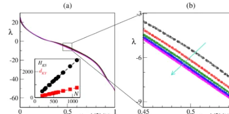
The single-scale L96 model (i.e., Eq. 1a) without the cou-pling to the fast scale) is no exception (Karimi and Paul, 2010; Gallavotti and Lucarini, 2014). Here we show that extensivity of chaotic behavior holds also in the two-scale model provided that – as discussed in Sect. 2.1 – the rela-tion (6) is satisfied. In the present context, the total number Nof degrees of freedom is controlled by two separate indica-tors,KandJ, so that, in principle, one can define two distinct thermodynamic limits, i.e.,K→ ∞andJ→ ∞. However, in practice, as long asK, J1, the spectral shape depends only onN alone, as seen in Fig. 1, where several different LSs nicely overlap.
In order to appreciate the different role ofK andJ, it is necessary to zoom in, as shown in Fig. 1b, where the re-gion characterized by a larger spread is displayed. The single spectra are grouped into five different branches, each corre-sponding to three different values ofK(K=18, 24 and 36, respectively marked as circles, squares and triangles) and to 3Actually, it is customary to defineρas(i−1/2)/N to reduce the amplitude of finite-size corrections (Pikovsky and Politi, 2016).
Figure 1.Extensivity of chaos.(a)Lyapunov spectra as functions of the rescaled indexir=(i−1/2)/NforK=18, 24 and 36 andJ= 10, 15, 20, 25 and 30 (all possible combinations).(b)Details of the central regionir∈(0.45,0.55). The cyan arrow marks the direction of increasingJ values, while eachJbranch is the superposition of the spectra forK=18 (circles),K=24 (squares) andK=36 (tri-angles). Inset of panel(a): Kolmogorov–Sinai entropyHKS(black circles) and Kaplan–Yorke dimensiondKY(red squares) as a func-tion of the number of degrees of freedomN=K(J+1). The dashed lines mark a linear fit with zero intercept and slope≈2.6 (HKS) and≈0.7 (dKY). Simulations have been performed withh=1 and
b= √
10J(see main text).
the sameJ. AsJ increases from 10 to 30, these branches converge to a limiting spectrum, which corresponds to the double thermodynamic limitK, J→ ∞. The indistinguisha-bility of the spectra obtained for the sameJ shows that K-type finite-size corrections are very small for the givenK; this is not a surprise, since the number of fast variables,KJ, is much larger than that of the slow variables,K.
The existence of a limit spectrum implies that the Kolmogorov–Sinai entropyHKS – a measure of the diver-sity of the trajectories generated by the dynamical system – is proportional to the numberNof degrees of freedom. This can be appreciated in the inset of Fig. 1a (see the black cir-cles), whereHKSis determined through the Pesin formula, which provides an upper bound toHKS(Eckmann and Ru-elle, 1985),
HKS= X
λ>0
λi. (19)
Similarly, the dimension of the attractor, i.e., the number of “active” degrees of freedom, is proportional toN, as seen again from Fig. 1a, where we have plotted the Kaplan– Yorke dimensionDKY (see red squares; Eckmann and Ru-elle, 1985):
DKY=M+ P
i≤Mλi |λM+1|
, (20)
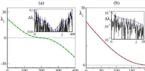
Figure 2. (a) Lyapunov spectrum for the conservative setup in Eqs. (8a) and (8b). Parameters are b=10, K=36 and J=10 (N=396 LEs), and initial conditions are chosen such that the con-served energy isE=36. The black solid line corresponds toh=1, while the dashed green line corresponds toh= −1; in the inset, the absolute difference1λibetween the two LSs is compared with one standard error in our numerical estimate (blue dashed line).(b)The second half of the Lyapunov spectrum (i∈ [199,396]; red dashed line) is folded under the reflection transformationλi→ −λN−i+1 over its first half (i∈ [1,198]; black solid line); in the inset, the ab-solute difference1λi between LS and its folded transformation is compared with one standard error in our numerical estimate (dashed blue line).
have chosenE=36 – see Eq. 9)4. Moreover, from Fig. 2b, we can appreciate that the LS is perfectly symmetric, since the second half of the spectrum superposes to the first half under the transformation λi → −λN−i+1 within numerical precision. This symmetry is an unexpected general property, which holds for any choice ofh,candb. In fact, the conser-vation law can only account for the existence of an extra zero-Lyapunov exponent. The overall symmetry of the LS must follow from more general properties such as the symplectic structure of the model or invariance under time reversal of the evolution equations. Unfortunately, this model is known to possess no symplectic structure, even if the energy is con-served (Blender et al., 2013), and the only symmetry we have been able to find is the invariance under the transformation t→ −t,Xk→ −Xk andYk,j → −Yk,j, accompanied by a change of the coupling constanth. Indeed, the green dashed line in Fig. 2a shows that the Lyapunov spectrum is invari-ant under the transformationh→ −h. Therefore, the overall symmetry remains an unexplained property.
3 Slow tangent-space bundle
3.1 Projection of CLVs in theXsubspace
We now come to the central result of this paper, namely the existence of a nontrivial subspace in tangent space associated with the slow dynamics of the L96 model.
4The invariant measure is absolutely continuous with respect to the Lebesgue one in the energy shell.
The individual LEsλi represent the average growth rate (and thus the inverse of suitable timescales) of well-defined small perturbations aligned along the corresponding CLV,vi. It is therefore logical to ask which of these “fundamental” perturbations are more relevant for the evolution of the ac-cessible macroscopic observables. In the present case, it is natural to focus our attention on the alignment along the slow variablesXk.
The norm of the (rescaled)ith CLV can be written as
||δX(i)||2+ ||δY(i)||2=1, (21) where the two addenda represent the squared Euclidean norm of the projection onto the slow and fast variables, δX(i)=(δX1(i), . . ., δXK(i))andδY(i)=(δY1(i),1, . . .δYK,J(i) ), re-spectively. The most natural indicator of how much theith CLV projects on the slow modes is thus theX-projected norm φi ≡ ||δX(i)||2.
However, it should be noted that, although the CLVs are intrinsic vectors, their mutual angles do depend on the rela-tive scales used to represent the single variables and, in par-ticular, fast and slow ones. If we change the units of measure used to quantify the fastY variables, introducingVj=γ Yj, the (Euclidean) norm of theith CLV becomes
L=φi+γ2(1−φi) .
As a result, in the new representation, the weight of the pro-jection onto the slow variables becomes
φi0=φi
L ,
which shows how the amplitude of the projection depends on the relative scale used to measure fast and slow variables. Since in the very definition of energy (see Eq. 9),XandY variables are weighted in the same way, it is natural to main-tain the original definition, i.e., to assume thatγ =1. Never-theless, as we will see while discussing the evolution of finite perturbations, the relative scale is an important parameter we can play with to extract useful information.
Given the strong temporal fluctuations ofφi(t )when the vectors are covariantly transformed along a trajectory (see the end of this section), it is convenient to refer to its time average (which, assuming ergodicity, corresponds to an en-semble average over the invariant measure),
Figure 3.CLV projection onto the slow variables.(a)CLV average projection norm8i of the CLVs (see text) as a function of the vec-tor index forK=36,J=10 andb=10 upon varying the coupling constanth. The upper part of(b)is the same as in(a)but in a log-arithmic scale vertical scale; in the bottom part of the panel are the corresponding Lyapunov spectra.
In fact, only a “central band” constituted by the CLVs asso-ciated with the smallest LEs displays a significative projec-tion over the slow variables. Note, however, that the typical LEs associated with the central band CLVs are clearly finite and are deemed “small” only in a relative sense, i.e., when compared with the largest positive and negative exponents of the full spectrum. For instance, for h=1/4, we can ap-proximately estimate the corresponding portion of the LS to extend between a magnitude of 2 and−5. We will comment further on this point in Sect. 4.
Note also that the CLV associated with the only null LE (in the following we simply denote it as the 0-CLV) displays a sharp peak of the projection norm8i. This is just a con-sequence of the delocalization of this CLV: the perturbation corresponding to the zero exponent points exactly along the trajectory. Direct integration of the phase-space equations (not shown) confirms that the total variability of the slow variables is of the same order of magnitude as the total vari-ability of the fast ones. This central band of CLVs defines the tangent-space slow bundle relevant for this paper. It be-comes more sharply defined for small values of the coupling h, but it keeps approximately the same position and width as the coupling his increased. In particular, for this set of pa-rameter values, this nontrivial slow bundle extends in tangent space over roughly 120 CLVs, much more than theK=36 slow degrees of freedom. The extension of the slow bundle can be better appreciated in Fig. 3b, where the time-averaged projections are shown on the logarithmic scale (top part of panel) and compared with the full spectrum of LEs (bottom part of panel).
We are interested in the dependence of this bundle on the number of slow and fast variables. As discussed in the pre-vious section, the L96 model is extensive in both the slow and fast variables, provided that the ratiof =J c/b2is kept constant (for the standard choice of parameters c=10 and f =1, so that it is sufficient to set b=
√
10J). In the
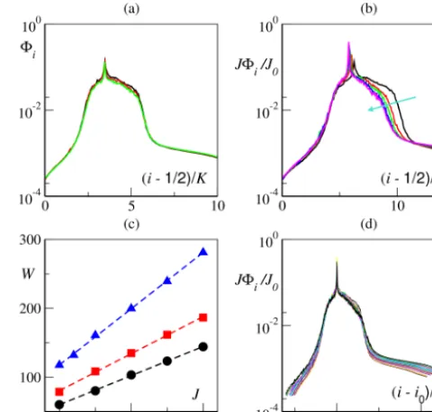
fol-Figure 4. Slow-bundle scaling forh=0.5 and f=1. (a) CLV time-averaged X-projected norm 8i forK=18, 24 and 36 and
J=10 vs. the rescaled index(i−0.5)/K.(b)Rescaled (see main text) CLV average projection norm8iforK=18 andJ=10, 15, 20, 25 and 30 (increasing along the cyan arrow) vs. the rescaled index(i−0.5)/J. A lack of precise collapse can be appreciated on the rightmost side of the central band.(c)Central band widthW(see main text for details) as a function ofJforK=18 (black circles),
K=24 (red squares) andK=36 (blue triangles). The best lin-ear fits, marked by the dashed lines, areW=18(1)+4.20(5)J(for
K=18),W=26(2)+5.4(1)J(K=24) andW=36(2)+8.2(2)J
(K=36).(d)Rescaled CLV average projection norm8i forK= 18, 24 and 36 andJ=10, 15, 20, 25 and 30 (all combinations) vs. the rescaled index(i−i0)/Ns. Herei0is the index of the 0-CLV and
Ns=K(1+αJ ), withα≈0.22 (see text). We choose the vertical axis rescaling reference asJ0=10.
lowing we present results forh=0.5, but we have carefully verified that analogous results hold for other values of the coupling constanth.
We first setJ=10 and explore the behavior of the slow bundle whenK is varied (note that no parameter rescaling is required while changing K). Our simulations, reported in Fig. 4a, clearly show that the slow bundle is extensive with respect toK: upon rescaling the vector index as i→
(i−0.5)/K, we observe a clear collapse of the projection patterns.
Xnorm to be inversely proportional toJ. The projection data reported in Fig. 4b indeed show a convincing vertical col-lapse of the rescaledXnorm8iJ /J0(here we fix a reference J0=10), but accompanied by a shrinking of the central band on the right side, asJis increased.
In order to accurately determine the width of the central band, i.e., the slow-bundle dimension, we fix a threshold for therescaledXnorm,J 8i/J0=10−2and estimate the num-berNsof CLVs with a projection above such a threshold (we have verified that our results hold within a reasonable range of thresholds). The resulting widthsNs(K, J ), computed for different numbers of slow variables K, are summarized in Fig. 4c, where they are plotted versusJ. For the fixedK, we see a clear linear increase, compatible with the law
Ns(K, J )=K (1+αJ ) , (23) where the coefficientαdepends on the values ofh,c,Fsand Ff. In the present case, a best fit gives α≈0.22. The most general representation of the projections is finally obtained by rescaling the index according toNs and by using the 0-CLV (which corresponds to the peak of8i) as the origin of the horizontal axis. The excellent collapse in Fig. 4d con-firms the extensivity of the slow bundle with bothKandJ. The slow bundle is not a simple representation of theX sub-space: it does not coincide with the slow variables themselves but involves also a finite fractionαof the fast ones, singling out a fundamental set of tangent-space perturbations closely associated with the slow dynamics. The origin of the phe-nomenological scaling law (23) will be discussed in the next section.
Before concluding this section, we would like to briefly discuss the time-resolved projected norm φi(t ). So far, we have discussed time-averaged quantities, but it is worth men-tioning that the X projections of individual CLVs are ex-tremely intermittent, hinting at a complex tangent-space flow structure.
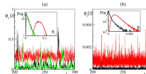
In Fig. 5a we display a few selected time series of the norm φi(t ) for b=10, K=36, J=10 and h=1/4 (the overall picture does not change qualitatively for different choices of the coupling strength). The time series correspond to the 110th vector, located in the left part of the central band (before the 0-CLV), the 160th vector, located in the right part, and the 0-CLV (vector indexi=122). We clearly see a strong intermittency, resulting in a very skewed distribution of the time-resolved Xnorms. The 0-CLV is an exception, displaying more regular oscillations and a rather symmetric distribution around its mean value. This confirms the pecu-liar nature of the 0-CLV, whose delocalized structure is es-sentially determined by its alignment with the phase-space flow.
In Fig. 5b we display vectors outside the slow bundle: the 1st and the 250th, which are on the left- and right-hand side of the central band, respectively. We see that also vectors out-side the slow bundle display a certain degree of intermittency, albeit on a faster timescale, and rather skewed distributions of
Figure 5.Time trace and probability distribution of CLV instan-taneous projection in theXsubspace forh=1/4 andb=10 and
K=36 andJ=10.(a)Slow-bundle vectors,i=110 (black line),
i=122 (red line, the 0-CLV) andi=160 (green line). In the in-set are the corresponding probability distributions of the three CLV time traces.(b)For two other CLVs with negligibleXprojection, first vector (black line) and 255th vector (red line). In the inset are corresponding probability distributions of the two CLV time traces.
theirφi(t )values. TheirXprojection, of course, is strongly suppressed and remains very close to 0. In Sect. 4, we will further comment on the intermittent behavior ofφi(t ), show-ing that it arises from near degeneracies in the instantaneous instability rates.
4 The origin of the slow bundle
In the previous section, we have identified a slow bundle in the tangent space of the L96 model – a central band centered around the 0-CLV – whose covariant vectors are character-ized by a large projection over the slow degrees of freedom. It is natural to expect this band to be associated not only with long timescales (i.e., the inverse of the corresponding LEs) but also with large-scale instabilities.
We begin by discussing the pedagogical example of the uncoupled limit (h=0). In this case, the X andY subsys-tems evolve, by definition, independently, and one can sep-arately determineK LEs associated with the slow variables andKJexponents associated with the fast variables. The full spectrum can be thereby reconstructed by combining the two distinct spectra into a single one. The result is illustrated in Fig. 6a, where the red crosses correspond to theXLEs. Note that the same area is also spanned by the central part of the fast-variable spectrum. The region covered by the slow LEs, where the instability rates of the two uncoupled systems have the same magnitude, roughly corresponds to the location of the slow bundle in the coupled-model CLVs spectrum. This suggests that the origin of the slow bundle can be traced back to a sort ofresonancebetween the slow variables and a suit-able subset of the fast ones.
there-fore, is strictly equal to either 0 or 1, depending on the vector type, and can be used to distinguish the two types of vec-tors when the full set of (uncoupled) equations is integrated simultaneously.
We now proceed to discuss the coupled case. When the coupling is switched on, it has a double effect: (i) it modi-fies the overall dynamics, i.e., the evolution in phase space, in Eqs. (1a) and (1b), and (ii) it directly affects the tangent-space evolution, in Eqs. (18a) and (18b), destroying the block diagonal structure of the uncoupled Jacobian matrix. This, in turn, prevents one from identifying single LEs with ei-ther the slow or the fast dynamics. In order to be able to also distinguish the two contributions in theh >0 case, we study an intermediate setup characterized by a full coupling in real space but remove it from the tangent-space dynam-ics. In practice, we simulate the full nonlinear model (1a and 1b) and use the resulting trajectories to “force” an un-coupledtangent-space dynamics, that is
δX˙k=δXk−1(Xk+1−Xk−2)
+Xk−1(δXk+1−δXk−2)−δXk, (24a) δY˙k,j =cb
δYk,j+1(Yk,j−1−Yk,j+2)
+Yk,j+1(δYk,j−1−δYk,j+2)−cδYk,j, (24b) where the coupling terms, proportional to h in Eqs. (18a) and (18b), have been ignored. This way, the Jacobian matrix is still block diagonal.
Thanks to this approximation, we can define tworestricted
spectra λXk andλYj for the slow and fast variables, respec-tively, and thereby recombine them into a single spectrum by ordering the exponents from the largest to the most negative one. A comparison between the resulting reconstructed spec-tra and the full ones (with coupling acting both in real and tangent space) shows an excellent agreement, at least in the rangeh∈(0,1). Two examples forh=1 andh=1/16 are given in Fig. 6b, while the dependence of their root-mean-square difference1λR onhis reported in Fig. 6c (blue di-amonds). It is not, however, clear to what extent this is a general property of high-dimensional dynamics; we are not aware of similar analyses made in high-dimensional models. The modifications induced by real-space coupling are more substantial. They can be quantified by computing the root-mean-square differences
1λX(h)= v u u t 1 K
K X
k=1 h
λXk(h)−λXk(0)i2, (25)
1λY(h)= v u u t
1 KJ
KJ X
j=1 h
λYj(h)−λYj(0)i2,
which measure the average variation in the restricted spec-tra upon increasing the coupling. Numerical simulations, re-ported in Fig. 6c, show that both1λXand1λY increase ap-proximately linearly withh, the main difference being that
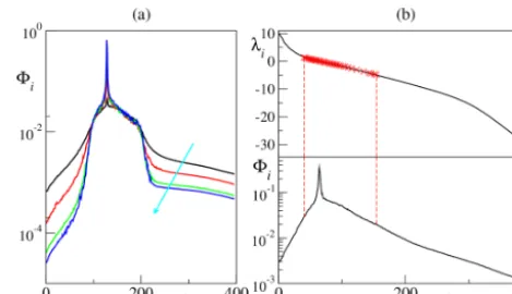
Figure 6. (a)Lyapunov spectra for the uncoupled (h=0) case de-composed in its slow (λX; red crosses) and fast (λY; black solid line) parts.(b)Full Lyapunov spectra (full lines) superimposed with spectra reconstructed from their restricted (see text) counterparts (dashed lines) forh=1 andh=1/16.(c)Root-mean-squared dif-ference between the finitehrestricted spectra and the completely uncoupled fast and slow spectra, for both fast (black squares) and slow (red circles) dynamics. Power law fits (dashed lines) return slopes close to unity (respectively≈0.9 and≈1.1), suggesting a simple linear growth with the couplingh. Blue diamonds refer to the root-mean-square difference1λRbetween the full LS and the reconstructed ones in the restricted tangent-space approximation. Both axes are represented in a double logarithmic scale. In the up-per part of(d)is an enlarged view of the central part (i∈ [50,250] of the restricted spectra forh=1/8, with the slow (λX, red crosses) and fast (λY, black solid line) components differently marked. In the lower part of the panel is the same enlarged view of theh=1/8 projection norm, as computed from the fully coupled dynamics. The vertical red dashed lines mark the upper (iL) and lower (iR) bound-aries of the superposition region as reported in Table 1. In all panels, we have fixed the following:b=10,K=36 andJ=10.
over the entire central band. This means that the orientation of the CLVs is very sensitive to the coupling itself.
The main mechanism responsible for the reshuffling of the CLV orientation is the (multifractal) fluctuations of finite-time LEs (Pikovsky and Politi, 2016). Fluctuations are the unavoidable consequence of the different degrees of stabil-ity experienced in different regions of the phase space, and they occur in both strictly hyperbolic and nonhyperbolic dy-namical systems, although they are typically much larger in the latter context. Fluctuations may be so large as to bridge the gap between distinct LEs, which results in a lack of dom-ination of the Oseledets splitting (Pugh et al., 2004; Bochi and Viana, 2005) and in the sporadic occurrence of near tan-gencies between pairs of different CLVs (Yang et al., 2009; Takeushi et al., 2011)5. Fluctuations are also responsible for the so-calledcoupling sensitivity(Daido, 1984; Pikovsky and Politi, 2016): strictly degenerate LEs in uncoupled systems may separate by an amount of the order of 1/|lnε|, whereε is the (small) amplitude of the coupling strength.
Let us be more quantitative and introduce the finite-time Lyapunov exponents γi(t ), computed from the average ex-pansion rate over a window of lengthτw,
γi(t )= 1 τw
ln||M(xt, τw)vi(t )||, (26)
whereM(xt, τw)is the propagator (15) for the tangent-space evolution over time τw, while the CLVs vi is normalized to unity. Their asymptotic time average obviously coincides with the corresponding LEs,hγi(t )it≡λi.
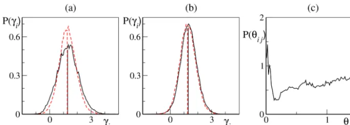
We are interested in the probability distributionP (γi)of γi, obtained by evolving a long trajectory. For short times, γi fluctuations significantly depend on the coordinates used to parametrize the dynamics, but upon increasing τw, such a variability is progressively lost and the width of P (γ ) scales as 1/√τw, as prescribed by the multifractal formal-ism (Pikovsky and Politi, 2016). In the following, we have set τw=0.5, after having verified that it is long enough. Here, for illustrative purposes, we have selected two vectors which, in the absence of tangent-space coupling, are of the XandY type, respectively6. From Fig. 7a, it is clear that the amplitude of the fluctuations largely exceeds the difference between the corresponding mean values (i.e., the asymptotic LEs; see the vertical straight lines) and that the same holds true after restoring the coupling in tangent space (Fig. 7b).
Consistently, in Fig. 7c, we show that the corresponding CLVs are characterized by nonnegligible near tangencies: 5Perfect tangencies may occur, but only for a set of zero-measure initial conditions, such as the homoclinic tangencies in low-dimensional chaos.
6Given the two restricted spectraλX
k andλYj, they are combined into a single set of ordered LEs and labeled according to the indexi. Depending whether theith exponent belongs to theXorYrestricted spectra, we conclude that the correspondingith CLV in the fully coupled spectrum is of theXorY type.
The probability distribution of the relative angle,
θi,j(t )=arccosvi(t )·vj(t ), (27) indeed exhibits a peak near 0.
We have verified this to be the generic behavior, as ex-pected due to the nonhyperbolic nature of the L96 model. The near tangencies between different CLVs within the slow bundle provide strong numerical evidence of the mixing be-tween slow and fast degrees of freedom and are perfectly consistent with the nonnegligible projection onto the slow X subspaces of all vectors in the slow bundle. In fact, in the presence of two similarly unstable directions, the cor-responding CLVs tend to wander in a (fluctuating) two-dimensional subspace, selecting their current direction on the basis of the relative degree of instability. It is therefore natu-ral to expect that, in the presence of strong fluctuations, an X-type vector (in the uncoupled limit) temporarily aligns along theY directions and vice versa, thereby giving rise to a pro-jection pattern such as the one seen in the central region of the CLVs spectrum, where all vectors have a nonnegligible average projection over theXdegrees of freedom.
The intermittent nature of the instantaneousXprojection φi(t )discussed in Sect. 3.1 further validates this picture: it is the result of the large fluctuations exhibited by finite-time LEs, which are, in turn, associated with changes of direc-tions when the CLV comes close to tangencies. Furthermore, the large ratio between the amplitude of the fluctuations and the separation between consecutive LEs suggests that this ex-change of directions may extend beyond the nearest neigh-bors along the spectrum. We conjecture that the relatively smooth boundary of the central band is precisely a manifes-tation of this sort of extended interaction.
Finally, we return to the restricted LEs to see whether – as implied by the above conjecture – their knowledge can help to identify the slow-bundle boundaries. In practice, we have first identified the borders of the region covered by both slow LEs. They are given by the indices (within the reconstructed spectrum) of the largest and smallest restricted slow LE, la-beled, respectively, asiL and iR. They are reported in Ta-ble 1, together with the corresponding value of the restricted Lyapunov exponent, for different coupling values. The agree-ment with the actual boundaries of the slow bundle – as re-vealed by a visual inspection of the projection patterns8i – is actually pretty good (see, e.g., Fig. 6d forh=1/8).
Altogether, our analysis suggests that coupling in real space induces a sort of “short-range” interaction within tan-gent space: each LE (and the corresponding CLV) tends to affect and be affected by exponents with a similar magnitude and thereby characterizes a similar degree of instability in a sort of resonance phenomenon.
Figure 7. (a–b)Probability distribution of the finite-time LEs (26) for two nearby LEs belonging to the slow bundle. We show results for the 92nd (black solid line) and 93rd (red dashed line) LEs which, in the absence of tangent-space coupling (the restricted setup; see text), belong, respectively, to theλXandλY restricted spectra.(a)Finite-time LEs fluctuations in the restricted case. The vertical lines mark the mean valuesλX92=1.30 andλY93=1.275 (indices refer to the full spectrum position, and they correspond to the 5th and 88th, respectively, LE in theXandYrestricted spectra).(b)Finite-time LEs fluctuations in the fully coupled case. The vertical lines mark the mean valuesλ92=1.31 andλ93=1.25.(c)Probability distribution of the angleθij(see Eq. 27) between the two corresponding CLVs in the fully coupled case. All simulations have been performed forK=36,J=10,b=10 andh=1/16. We have fixed the following in all panels:K=36 andJ=10.
Table 1.X-restricted largest (λX1) and smallest (λXK) LE with the corresponding full spectrum indices (iLandiR). All data refer to
b=10,K=36 andJ=10.
h λX1 λXK iL iR 1 1.33 −4.57 104 192 1/2 1.89 −5.18 93 197 1/4 2.13 −5.42 85 198 1/8 2.23 −5.53 80 199 1/16 2.29 −5.58 77 199
5 Finite perturbations
So far we have studied the geometry of the L96 model, deal-ing exclusively with infinitesimal perturbations. A legitimate question is whether we can learn something more by looking at finite perturbations.
Finite-size analysis has been implemented in the L96 model since its introduction (Lorenz, 1996), and it has been formalized with the definition of the so-called finite-size Lya-punov exponents (FSLEs; Aurell et al., 1997). In a nutshell, the rationale for introducing FSLEs is – as already recog-nized by Lorenz – that in nonlinear systems the response to finite perturbations may strongly depend on the observa-tion scale. Dropping the limit of vanishing perturbaobserva-tions, of course, weakens the level of mathematical rigor of the in-finitesimal Lyapunov analysis, but it nevertheless allows for a meaningful study of the underlying instabilities.
Here, we follow the excellent review (Cencini and Vulpi-ani, 2013), where applications to L96 were also discussed. Given a generic trajectory x(t ), the idea is to define a se-ries of thresholds δn=δ0σn, with σ >1, and to measure the times τ (δn)needed by the norm of a finite perturbation 1x(t )=x0(t )−x(t )to grow from the amplitudeδntoδn+1.
The FSLE3(δn)is then defined as 3(δn)=
lnσ
hτ (δn)i
, (28)
whereh·idenotes an average over many realizations of the perturbation. In practice, one starts at time t0 with a finite perturbation k1x(t0)k δ0 to ensure a correct alignment (along the most expanding direction) by the time the pertur-bation amplitude reaches the first thresholdδ0. Subsequently, both trajectoriesxandx0are followed, registering the cross-ing times of all δn thresholds. By repeating this procedure many times, one is able to estimate the FSLEs for all am-plitudesδn via Eq. (28). The FSLE in principle depends on the norm used to define the size of the perturbation (Cencini and Vulpiani, 2013). However, by construction, for vanishing perturbations, the FSLE should coincide with the largest LE, regardless of the norm:
lim δ→03(δ)
=λ1. (29)
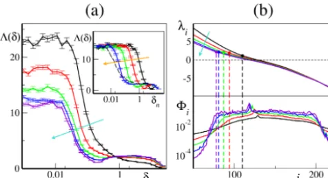
Figure 8. FSLE analysis.(a)FSLEs for different coupling con-stants,h=1 (black line),h=1/2 (red line),h=1/4 (green line),
h=1/8 (blue line) andh=1/16 (red line) – decreasing along the cyan arrow – vs. the finite-size amplitudes δn for theγ=10−3 norm. In the inset are the FSLEs forh=1/4 and differentγnorms (γ=1, 10−1, 10−2and 10−3, decreasing along the orange arrow). The error bars measure one standard error. The black dashed line marks the FSLEs for the limiting caseγ→0. Note the logarithmic scale for the abscissa of both graphs.(b)Details of the LE spectrum (top part of panel) and of the8i average projection norm patterns (bottom part of panel) as in Fig. 3b. The solid dots and the vertical dashed line mark the value and the location of the LEsλiSas
iden-tified in Table 2 (see main text for more details). Different coupling constant values are color-coded as in panel(a), withhdecreasing along the cyan arrow in the top part of the panel.
In this section we repeat this analysis in our setup, compar-ing the behavior of the FSLE with the analysis of the tangent-space slow bundle. In the following we use our standard pa-rameters (K=36,J=10 andb=10), using σ=
√
2 and δ0=10−3 and averaging the crossing times over 103 real-izations. For each realization, the initial finite perturbation (1X1, . . ., 1XK, 1Y1,1, 1YK,J)is chosen at random, with an initial amplitude of 10−5.
As we expect the FSLE to depend on the norm, we have decided to transform this weakness into an advantage by studying the behavior of an entire family of Euclidean norms, thereby extracting useful information from the dependence on the chosen norm. More precisely, we introduce the γ -dependent norm
k·kγ= s
X
k
X2k+γX k,j
Yk,j2 , (30)
which, for γ=1, coincides with the standard Euclidean norm. We considerγ ∈(0,1], a choice which allows explor-ing a broad range of weights of the slow variables.
In the inset of Fig. 8a, we see that the main effect of chang-ing the norm is a variation in the length of the two plateaus: upon decreasing γ, the first plateau shrinks, leaving space for a longer second plateau. The height of the two plateaus is largelyγ independent. This behavior can be qualitatively understood as follows. At early times, all components of the perturbation grow according to the maximum LE, which we
Table 2.Estimated slow dynamics finite-size instability3s(h) com-pared to the closest LE and its indexiSfor different coupling con-stants. Numbers in parenthesis refer to the uncertainty in3Sand, accordingly, ofiS. Results of the restricted analysis carried on in Sect. 4 are reported from Table 1 for comparison. All data have been obtained withb=10,K=36 andJ=10.
h 3s λiS iS λ
X 1 iL 1 1.2 (3) 1.15 110 (6) 1.33 104, 1/2 1.86 (11) 1.90 94 (2) 1.89 93, 1/4 2.07 (8) 2.04 87 (1) 2.13 85, 1/8 2.16 (11) 2.15 81 (1) 2.23 80, 1/16 2.2 (1) 2.18 78 (1) 2.29 77.
know from the previous analysis to be mostly controlled by the dynamics of the fastY variables. As time goes on, the perturbations of theY variables start saturating, while those of the slow variables keep growing, however, at a pace con-trolled by their (weaker) intrinsic instability. Upon decreas-ingγ, the relative weight of the less unstable, slow variables increases. However, there is a limit: even whenγ→0, the growth rate of theX perturbations is initially controlled by the fast variable. The range of this initial, approximately lin-ear regime depends on the initial amplitude of the fast com-ponents; this limit corresponds to the dashed curve in the in-set of Fig. 8a.
The FSLEs obtained for different coupling parametersh are shown in Fig. 8a, all for γ=10−3. Two plateaus are clearly visible, at least forh <1. The first one coincides with the maximum LE of the whole system, as per Eq. (29). The second one approximately extends over a range of 1 order of magnitude (at large scales, the plateau is obviously limited by the attractor size). Its height corresponds to the character-istic instability3s(h)associated with the effective dynamics of the slow variables, as conjectured in Cencini and Vulpiani (2013).
For each coupling h, we estimated the corresponding 3s(h)as the average of3(δn)in the intervalδn∈ [1,10]and identified the closest LEλiS and its indexiSin the Lyapunov
spectra. The results of this procedure are summarized in Ta-ble 2 and compared with the results of the restricted analysis obtained in Sect. 4.
plateau becomes less sharply defined, up to the caseh=1, where it is practically impossible to define a threshold. Cor-respondingly, the boundaries of the slow bundle in tangent space, as defined by inspection of8i, also become less well defined.
Altogether, the slow-variable (large-scale) instability 3s emerging from the finite-size analysis roughly coincides with the upper boundary of the slow bundle (i.e., the LEs associ-ated with the CLVs with a relevant projection onto the Xk variables). Following the analysis of the restricted spectra carried out in the previous section,3sis also close to the first restricted LE associated with theX subspaceλX1, as shown in Table 2. The parameterγ proves to be useful in improving the accuracy of the two plateaus exhibited by the FSLEs.
It is remarkable that the analysis of a single pair of trajec-tories allows for extracting information about (at least) two different Lyapunov exponents. We conjecture that the lin-early controlled growth of small, finite perturbations stops as soon as the fast components saturate because of nonlin-earities. Afterwards, fast variables act as a sort of noise on the slow ones, whose dynamics is still in the linear regime. Finally, in view of the above-mentioned closeness between the restricted and fully coupled LS, it is reasonable to con-jecture that, since coupling does not play a crucial role in tangent space, the growth rate corresponds, in this second regime, to the maximal LE of the slow variables, as indeed observed. Our result supports an earlier conjecture of Cencini and Vulpiani (2013) concerning the existence of an effective lower-dimensional dynamics capturing the slow-variable be-havior.
6 Discussion and conclusions
Our analysis of the tangent-space structure of the L96 model has identified a slow bundle within the full tangent space. It is composed of the set of covariant Lyapunov vectors charac-terized by a nonnegligible projection over the slow degrees of freedom. Vectors in this set are associated with the smallest (in absolute value) LEs and thus with the longest timescales. We have verified that the number of such vectors increases linearly with the total number of degrees of freedom so that the slow-bundle dimension is an extensive quantity.
The upper and lower boundaries of the slow bundle are better defined for a weak couplingh. However, the rescaled formulation of L96 (see Eq. 4a) shows that the effective upward coupling (from the fast to the slow variables) is hf =hJ c/b2, thereby suggesting that an increase of the am-plitude separationbcan increase the sharpness of the slow-bundle boundaries even for large h. As reported in Fig. 9a, numerical simulations withh=1 and increasing values ofb actually confirm this intuition, indicating that a slow bundle can be clearly defined also in the strong coupling limit, pro-vided that the slow- and fast-scale amplitudes are sufficiently separated.
Figure 9. (a)X-projection patterns 8i for Lorenz 96 with fast-variable forcing (Ff=6), strong coupling h=1 and increasing (along the direction of the cyan arrow) values of amplitude sepa-ration,b=10, 20, 40 and 50.(b)Lyapunov spectrum (top part of panel) andX-projection patterns (bottom part of panel) for Lorenz 96 with no fast-variable forcing (Ff=0) and standard parameter values,h=1 andb=c=10. The red crosses mark the values of theX-restricted spectrum (see Sect. 4 for more details). System size isK=36 andJ=10 in both panels.
In order to clarify the origin of the slow bundle, we have introduced the notion of restricted Lyapunov spectra and ar-gued that the central region, where the CLVs retain a signi-ficative projection over both slow and fast variables, corre-sponds to the range where the restricted spectra overlap with one another. In this region, fluctuations of the finite-time LEs much larger than the typical separation between consecutive LEs lead inevitably to frequent “near tangencies” between CLVs, thereby mixing slow and fast degrees of freedom into a nontrivial set of vectors which carries information on both sets of variables.
Besides, we have found that coupling in tangent space weakly influences the actual LEs, provided that it is ac-counted for in real space. This is one of the reasons for the finite-size analysis being able to give information about the instability of the slow bundle (i.e., the correspondence be-tween the second plateau displayed by the FSLE and the up-per boundary of the slow bundle). Further investigations are necessary to put our consideration on firmer ground.
thor-ough study, preliminary simulations indicate that the signa-ture of a slow bundle can be found also in the classical setup for sufficiently strong coupling. In particular, as reported in Fig. 9b forh=1, one can see that the region of nonnegligible Xprojections of the CLVs again coincides with the superpo-sition region of the slow and fast restricted spectra.
As already mentioned, the slow bundle is identified as the set of CLVs with a nonnegligible projection onto the slow degrees of freedom. One might argue that the average pro-jection8on theXsubspace decreases withJ, being at best of the order of 1/J, i.e., the fraction of slow degrees of free-dom. However, what matters is not the actual value of8but rather the ratio between the height of the plateau and that of the underlying background. The scaling analysis reported in Fig. 4 shows that this ratio stays finite while increasing the number of fast variables.
Altogether, we conjecture that (i) the fast stable directions lying beyond the slow-bundle central region are basically slaved degrees of freedom, which do not contribute to the overall dynamical complexity, and (ii) the fast unstable di-rections act as a noise generator for the Y degrees of free-dom (their projection onto theXvariables being negligible, and they do not talk directly with the slow variables). There-fore, it is natural to conjecture that the two subsystems mu-tually interact only through the slow-bundle instabilities so that suitably aligned perturbations of the fast variables can affect the slow variables and vice versa (see also Vannitsem and Lucarini , 2016). While this is a mere conjecture to be ex-plored in future works, it suggests that (some) covariant vec-tors could be profitably applied to ensemble forecasting and data assimilation in weather and climate models. In particu-lar, it has already been shown that restricting variational data assimilation to the full unstable subspace can increase the forecasting efficiency (Trevisan and Uboldi, 2004; Trevisan et al., 2010). In the future, we would like to explore whether a data assimilation scheme restricted to the slow bundle only (which does not encompass the entire unstable space) can lead to further improvements in forecasting.
The mechanism discussed in Sect. 4, relying on the overlap of the two restricted Lyapunov spectra should be common in nonlinear multiscale systems; therefore we believe our find-ings to be fairly generic. In the future, it will be interesting to extend the present analysis of Lyapunov exponents and covariant Lyapunov vectors to models with multiple scales and/or higher complexity and relevance, such as the coupled atmosphere–ocean model MAOOAM (De Cruz et al., 2016), or simplified multilayer models of the atmosphere, such as PUMA (Fraedrich et al., 2005) or SPEEDY (Molteni, 2003), thus going beyond the LEs studies of De Cruz et al. (2018) to include the full tangent-space geometry.
Data availability. All data have been generated by numerically
in-tegrating the model equations mentioned in the paper. While all
al-gorithmic details are duly given in our paper, in case of future needs, the authors are willing to provide their numerical codes on request.
Author contributions. AP and FG devised the research, MC is
re-sponsible for the simulations, and all authors analyzed the data and wrote the paper.
Competing interests. The authors declare that they have no conflict
of interest.
Acknowledgements. Francesco Ginelli warmly thanks
Mas-simo Cencini for truly invaluable early discussions. We ac-knowledge support from EU Marie Skłodowska-Curie ITN grant no. 642563 (COSMOS). Mallory Carlu acknowledges financial support from the Scottish Universities Physics Alliance (SUPA) as well as Sebastian Schubert and the Meteorological Institute of the University of Hamburg for the warm welcome and the stimulating discussions. Valerio Lucarini acknowledges the support received from the DFG Sfb/Transregion TRR181 project and the EU Horizon 2020 projects Blue-Action (grant agreement number 727852) and CRESCENDO (grant agreement number 641816).
Review statement. This paper was edited by Amit Apte and
re-viewed by two anonymous referees.
References
Abramov, R. V. and Majda, A.: New approximations and tests of linear fluctuation-response for chaotic nonlinear forced-dissipative dynamical systems, J. Nonlinear Sci., 18, 303–341, https://doi.org/10.1007/s00332-007-9011-9, 2007.
Aurell, E., Boffetta, G., Crisanti, A., Paladin, G., and Vulpiani, A.: Predictability in the large: an extension of the concept of Lya-punov exponent, J. Phys. A, 30 1, https://doi.org/10.1088/0305-4470/30/1/003, 1997.
Benettin, G., Galgani, L., Giorgilli, A., and Strelcyn, J. M.: Lyapunov characteristic exponents for smooth dynam-ical systems and for Hamiltonian systems; a method for computing all of them. Part 1: Theory, Meccanica, 15, https://doi.org/10.1007/BF02128236, 1980.
Berner, J., et al.: Stochastic parametrization: Toward a new view of weather and climate models, B. Am. Meteorol. Soc., 98, 565, https://doi.org/10.1175/BAMS-D-15-00268.1, 2017.
Blender, R., Lucarini, V., and Wouters, J.: Avalanches, breathers, and flow reversal in a continuous Lorenz-96 model, Phys. Rev. E, 88, 013201, https://doi.org/10.1103/PhysRevE.88.013201, 2013. Bochi, J. and Viana, M.: The Lyapunov exponents of generic volume-preserving and symplectic maps, Ann. Math., 161, 1423–1485, 2005.