https://doi.org/10.5194/esd-9-757-2018
© Author(s) 2018. This work is distributed under the Creative Commons Attribution 4.0 License.
Recent trends in the frequency
and duration of global floods
Nasser Najibi1,2,3and Naresh Devineni1,2,3
1Department of Civil Engineering, City University of New York (City College), New York, 10031, USA
2Center for Water Resources and Environmental Research (City Water
Center), City University of New York, New York, 10031, USA
3NOAA/Cooperative Science Center for Earth System Sciences and Remote Sensing
Technologies (CREST), City University of New York, New York, 10031, USA
Correspondence:Nasser Najibi ([email protected])
Received: 11 June 2017 – Discussion started: 4 July 2017 Revised: 7 April 2018 – Accepted: 16 May 2018 – Published: 8 June 2018
Abstract. Frequency and duration of floods are analyzed using the global flood database of the Dartmouth Flood Observatory (DFO) to explore evidence of trends during 1985–2015 at global and latitudinal scales. Three classes of flood duration (i.e., short: 1–7, moderate: 8–20, and long: 21 days and above) are also considered for this analysis. The nonparametric Mann–Kendall trend analysis is used to evaluate three hypotheses addressing potential monotonic trends in the frequency of flood, moments of duration, and frequency of specific flood duration types. We also evaluated if trends could be related to large-scale atmospheric teleconnections using a generalized linear model framework. Results show that flood frequency and the tails of the flood duration (long duration) have increased at both the global and the latitudinal scales. In the tropics, floods have increased 4-fold since the 2000s. This increase is 2.5-fold in the north midlatitudes. However, much of the trend in frequency and duration of the floods can be placed within the long-term climate variability context since the Atlantic Multidecadal Oscillation, North Atlantic Oscillation, and Pacific Decadal Oscillation were the main atmospheric teleconnections explaining this trend. There is no monotonic trend in the frequency of short-duration floods across all the global and latitudinal scales. There is a significant increasing trend in the annual median of flood durations globally and each latitudinal belt, and this trend is not related to these teleconnections. While the DFO data come with a certain level of epistemic uncertainty due to imprecision in the estimation of floods, overall, the analysis provides insights for understanding the frequency and persistence in hydrologic extremes and how they relate to changes in the climate, organization of global and local dynamical systems, and country-scale socioeconomic factors.
1 Introduction
Higher levels of vulnerabilities to extreme events, especially floods, are becoming a “new normal” in both developing and developed countries (Mirza, 2003; Thomalla et al., 2006). There is rapidly growing population, assets, and expanding residential and commercial sectors that are susceptible to damages during these events (Hallegatte et al., 2013; Singh and Zommers, 2014). Moreover, while flood-related fatali-ties have substantially decreased in recent decades mainly due to improved early warning systems and better flood
con-trol infrastructure, statistics still point out that there are peo-ple (in)directly affected by these events. For instance, Guha-Sapir et al. (2016) in their annual disaster statistical review of 2016 reported that the number of people affected by hy-drologic disasters (floods or landslides) is 78.1 million, ap-proximately 13.7 % of all people affected in 2016. It is also striking to note that 60 million of these 78.1 million people were affected by one flood in China.
dis-turbances in the food supply chain, undernutrition, water-/vector-borne diseases, and being injured, displaced, or left homeless) (Schultz, 2006; Milojevic et al., 2011; Lowe et al., 2013; Moftakhari et al., 2017). An unusual increase in the bacillary dysentery risk in Baise (Guangxi Province, China) during the years 2004 to 2012 is a case in point (see more details in Liu et al., 2017). The recent Thailand floods that occurred in July 2011 and December 2014 also caused severe supply chain disruptions (Ziegler et al., 2012; Haraguchi and Lall, 2015; Promchote et al., 2016).
Often, these impacts are magnified when the floods are due to persistent and recurrent rainfall. Such floods typically last longer (henceforth called long-duration floods) and are asso-ciated with repeated rainfall events in the regions. Recently, Robertson et al. (2011), Nakamura et al. (2013), Lu et al. (2013), Ward et al. (2015), Haraguchi and Lall (2015), Najibi et al. (2017), Gao et al. (2017), and Lu and Lall (2017) have attempted to quantify the causal mechanisms and impacts of such long-duration floods at the regional scale. An important question in this context is whether we understand the plan-etary nature of the trends in the frequency and duration of these long-duration floods. Understanding the global trends and quantifying their potential climate-related attributes can help improve flood forecasting systems and better manage flood control infrastructure.
Global and near-daily observations from the Earth’s sur-face are now available through satellite microwave sensors (active/passive), which are being employed to measure the changes of water surfaces (e.g., river discharge and water-shed runoff) (Brakenridge et al., 2007). Utilizing such infor-mation even with limited ground-based discharge data can allow the mapping of flood inundation extents at many lo-cations around the world. Such satellite-based measurements have a particular advantage in understanding the impacts of floods in developing nations where there is a lack of sufficient in situ measurements (Brakenridge et al., 2007; Van Dijk et al., 2016; Brakenridge et al., 2016). In this study, we pro-vide a global-scale analysis of the recent trends in the fre-quency and probability distribution of the duration of floods provided by such satellite imagery products with an objec-tive to understand the trends from the context of ocean– atmospheric interactions and socioeconomic factors.
Given the floods (especially the long-duration floods) are caused by a systematic organization of the global-to-local dy-namical systems of climate and atmosphere (Najibi et al., 2017), characterizing the underlying features of temporal trends, i.e., whether the trend is due to secular changes or due to low-frequency oscillations manifesting as periods of wet–dry phases (regime-like behavior) will help us better un-derstand the frequency and persistence in the organization of these systems. We can use this understanding to explore their predictability using state space models (Abarbanel and Lall, 1996; Karamperidou et al., 2014; Perdigão and Blöschl, 2015). Together, the characterization of the trends and the predictability of these extremes will enable us to improve the
climate impact assessment and understand whether or not a regional persistent flood regime is likely to end or continue.
Consequently, we utilized the global active archive of flood events (with 31 years of data from 1985 to 2015) to address the following five questions:
1. How has the annual frequency of floods changed at the global scale and various latitudinal belts during the last 3 decades?
2. How has the probability distribution of flood dura-tion (represented by the moments and extreme values) changed at the global scale and various latitudinal belts during the last 3 decades?
3. Are the changes (if any) in the flood frequency and the probability distribution of flood durations due to the changes in a specific flood class, i.e., short, moderate, or long duration?
4. Can the changes (if any) in the flood frequency and the probability distribution of flood durations be related to the variability in the atmospheric teleconnections and low-frequency climate oscillations?
5. Which countries are most vulnerable to short-, moderate-, and long-duration floods?
We address each question using a formal hypothesis-testing framework. This paper is organized as follows: Sect. 2 provides the detailed information about the global flood database, design hypotheses, and employed methodology in this study. Section 3 presents the results of the hypothesis tests and the country-scale vulnerability analysis to different flood durations. In Sect. 4, we present a generalized linear model (GLM) framework to investigate the potential causes of the observed trends and also discuss the other compara-ble global trend studies. Finally, we present the concluding remarks and highlights in Sect. 5.
2 Data, methodology, and hypotheses
2.1 Global active archive of flood events: Dartmouth Flood Observatory (DFO)
DFO mostly takes advantage of orbital remote-sensing sen-sors to identify, measure, and monitor global flood events by gathering globally consistent information on surface water changes, in particular since 1999. Floods are detected us-ing MODIS (Moderate-Resolution Imagus-ing Spectroradiome-ter) sensors (approximately 250 m footprint pixel), and river discharges are measures using satellite microwave data such as AMSR-E (Advanced Microwave Scanning Radiometer for Earth Observation System (EOS) from Global Change Observation Mission – Water, GCOM-W). The discharge values and runoff coefficients are then calculated from the Water Balance Model (WBM) embedded with the specific soil type, surface gradient, soil permeability, and land use– land cover (LULC) characteristics. These remote-sensing and model outputs are employed conjunctively to map the potential flood inundation extents frequently. Then, a num-ber is assigned to the flood if (a) it is unusually “large” com-pared to the typical annual high water and previously mapped water–land extents, and/or (b) if there are significant dam-ages caused to the structures, extensive land inundation, and fatalities (Brakenridge et al., 2016).
It is important to note that the quality of data has improved in recent times. The improvements in the level of media re-porting and information quality have improved the reliability of the data. At the same time, the likely improvements in the accuracy of in situ measurements, advances in satellite and ground-based sensors, data storage, and transfer facili-ties also contributed to the data quality. Moreover, Braken-ridge et al. (2003, 2005, 2012) have discussed that the fre-quent temporal sampling of satellite-based observations and ground sources (media reporting) determines the accuracy level amongst the (non-)flood event candidates. The dataset covers flood events at the global scale from 1 January 1985 to present. Any recent flood event is added immediately to the data archive. In this study, we considered 31 years of global flood events from 1 January 1985 to 31 December 2015. This comprehensive dataset includes information on the lo-cation of the flood events (longitude, latitude, and the name of the country), flood beginning and end dates, their dura-tion (which is the number of days between the flood be-ginning and end dates), and damages due the flood (which is an estimation of flood-induced damage according to all the relevant sources). It is reported by the DFO that occa-sionally when there is no flood beginning date mentioned in the news report, they assume middle of the month as the start date (http://floodobservatory.colorado.edu/Archives/ ArchiveNotes.html, last access: 1 March 2016). We verified the fraction of such events among the total events and found that less than 5 % (194 out of 4311 events globally over the 31 years) have such an assumption. We also explored the dis-tribution of the month of occurrence for the flood beginning and end dates across the globe. While investigating these records, it become apparent that the days 1, 5, 10, 15, 20, and 25 also have an increased number of flood counts (around 4 %), which suggests a reporting bias or a phenomenon of
rounding off to the nearest fifth day. While there was infor-mation on the phenomenon of rounding off to the middle of the month in the DFO data description, we did not find any relevant information on the pattern every fifth day. However, we did not find any systematic spatial pattern for these ap-parent reporting biases (see Appendix B for more details). The DFO is the only global dataset of observed flood events. Many of the prior studies either focused on rainfall-based datasets or model-based river flow data. In this regard, the present study adds a new dimension to the flood literature, especially the understanding of the long-duration floods at the global scale.
2.2 Aggregating floods on the basis of the latitudinal belts
The flood events are spatially aggregated to five climate
zones – tropics (23.5◦S to 23.5◦N), Northern Hemisphere
subtropics (23.5–35◦N) and midlatitudes (35–55◦N), and
Southern Hemisphere subtropics (23.5–35◦S) and
midlat-itudes (35–55◦S) (Environmental Literacy Council, ELC,
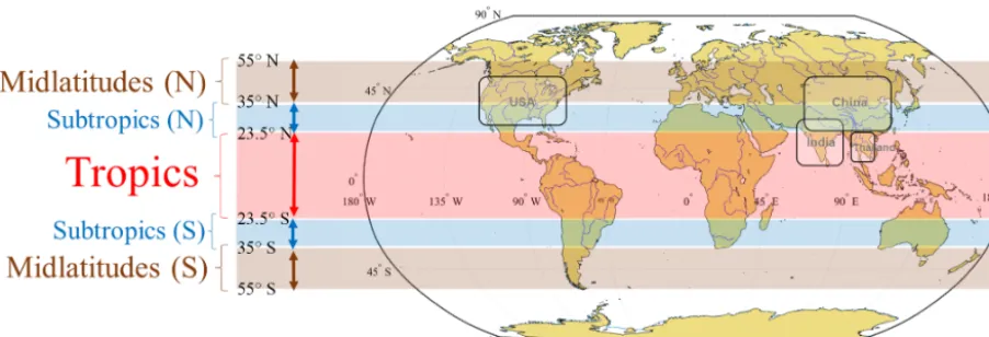
2015). We chose these spatial aggregations along the latitudi-nal belts to be consistent with the global circulation dynam-ics, zonally symmetric thermal forcing (Walker and Schnei-der, 2005; Zhai and Boos, 2015), temperature variabilities, and precipitation patterns (Gabler et al., 2008). In addition, such specifications will result in achieving higher coherency in satellite-based data acquisition in particular for the passive sensors because of varying solar reflectivity and ascending– descending satellite orbits along different latitudes (Thenk-abail, 2015). Figure 1 represents the schematic of the five cli-mate zones. We also show the geographical locations of four countries (United States, China, India, and Thailand) that have already experienced high rates of long-duration floods among all the countries from 1985 to 2015.
Next, for each latitudinal belt, the total number of floods per year (calendar year from 1 January to 31 December), the duration of these floods, and their location (name of country) are processed. This procedure is formulated as follows:
FCt,r=total number of flood event(s) in latitudinal beltr
and yeart [count(s)], (1)
Ft,Dr=duration(s) of flood event(s) in latitudinal beltr
and yeart[day(s)], (2)
Ft,Lr=location(s) of flood event(s) in latitudinal beltr
and yeart[name of country(ies)], (3)
whereFCindicates the flood counts (frequency), andFDand
FLdenote the vectors of flood duration and flood location for
each of these flood events, respectively. The superscriptsr
andtdenote the latitudinal belt (r= {global, tropics,
midlat-itudes (N and S), subtropics (N and S)}) and year (t= {1985,
Figure 1.Spatial segmentation to assign the global flood events (1985 to 2015) into different latitudinal belts: midlatitudes (N): 35–55◦N;
subtropics (N): 23.5–35◦N; tropics: 23.5◦S–23.5◦N; subtropics (S): 23.5–35◦S; and midlatitudes (S): 35–55◦S; (N) and (S) indicate
North-ern Hemisphere and SouthNorth-ern Hemisphere, respectively; the four rounded rectangles shows the United States of America (USA), China, India, and Thailand.
In addition, the number of floods in each latitudinal belt are also categorized in terms of their duration. We denote the event as a short-duration floodFCt,r
Sif the duration is between
1 and 7 days, moderate-duration floodFCt,r
Mif the duration is
between 8 and 20 days, and as a long-duration floodFCt,r
L if
the duration is greater than or equal to 21 days. These cate-gories are also consistent with the DFO’s flood classification (Brakenridge, 2016). The subscripts “S”, “M”, and “L” stand for short-, moderate-, and long-duration flood events, respec-tively.
2.3 Atmospheric teleconnections and climate indices
We used large-scale ocean–atmospheric teleconnections to investigate the extent to which the trends in the floods can be related to natural variability (Enfield et al., 2001; Ward et al., 2016) in the climate–atmospheric system. Since the climate system has as quasi-periodic nature that often man-ifests as wet and dry regimes, it is important to understand whether the trends, if observed, can be attributed to these nat-ural oscillations. Hence, we used the El Niño–Southern Os-cillation (ENSO), Pacific Decadal OsOs-cillation (PDO), North Atlantic Oscillation (NAO), and Atlantic Multidecadal Oscil-lation (AMO) as proxies for interannual, decadal, and multi-decadal climate variability.
We obtained 31 years (1985–2015) of ENSO data (aggre-gated based on the monthly anomalies of Niño 3.4) from the HadISST1 dataset (Rayner et al., 2003). Monthly AMO and PDO anomalies are obtained from the NOAA/Earth System Research Laboratory at http://www.esrl.noaa.gov/psd/data/ climateindices/list (last access: 1 March 2016) (Zhang et al., 1997), and then averaged to yearly time series from 1985 to 2015. Similarly, the monthly NAO indices are obtained from the NOAA/National Weather Service, Climate Pre-diction Center at http://www.cpc.ncep.noaa.gov/products/
monitoring_and_data/ (last access: 1 March 2016) (Barnston and Livezey, 1987; Hurrell and Van Loon, 1997) and aver-aged to yearly time series.
2.4 Calculating resistant metrics from the distribution of flood duration
In addition to the frequency of the floods (FCt,r), we
calcu-late a set of “resistant measures” to evaluate the existence of any significant monotonic time trend in the probability dis-tribution of flood duration. Four moment indicators are se-lected because of their scale-invariant characteristics suitable for such asymmetric distributions. These metrics include the median, median absolute deviation (MAD), resistant skew-ness, and the 90th percentile of the distribution of flood du-rations in each year. Each of these metrics is computed as a time series of 31 years (1985–2015) for each of the six spa-tial scales (i.e., global, tropics, midlatitudes – N, midlatitudes – S, subtropics – N, subtropics – S). It is straightforward to calculate the median and 90th percentile from the distribu-tion of flood duradistribu-tion each year. We explain the formuladistribu-tion and the properties of the other two metrics here.
2.4.1 Median absolute deviation (MAD) of flood durations
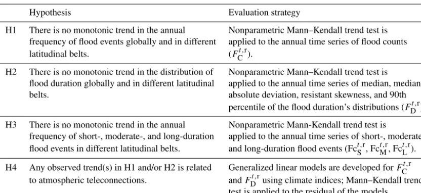
Table 1.Proposed hypotheses and evaluation approach.
Hypothesis Evaluation strategy
H1 There is no monotonic trend in the annual Nonparametric Mann–Kendall trend test is
frequency of flood events globally and in different applied to the annual time series of flood counts
latitudinal belts. (FCt,r).
H2 There is no monotonic trend in the distribution of Nonparametric Mann–Kendall trend test is
flood duration globally and in different latitudinal applied to the annual time series of median, median
belts. absolute deviation, resistant skewness, and 90th
percentile of the flood duration’s distributions (FDt,r).
H3 There is no monotonic trend in the annual Nonparametric Mann-Kendall trend test is
frequency of short-, moderate-, and long-duration applied to the annual time series of short-, moderate-,
flood events in different latitudinal belts. and long-duration flood events (Fct,Sr, Fct,Mr, Fct,Lr).
H4 Any observed trend(s) in H1 and/or H2 is related Generalized linear models are developed forFCt,r
to atmospheric teleconnections. andFDt,rusing climate indices; Mann–Kendall trend
test is applied to the residual of the models.
to SD, as it measures the deviation from the average flood duration. MAD is computed as follows:
Ft,Dr
MAD=median
F
t,r D −F
t,r DMedian
, (4)
where “t”, “r”, andFt,Dr are the same variables defined in
Eq. (2) and FDt,r
Median refers to the median of distribution of
flood duration.
2.4.2 Resistant skewness of flood durations
The presence of outliers amongst the variables will generate a large and possibly misleading measure of skewness (Helsel and Hirsch, 1992). Instead, the resistant skewness is a more robust measure for capturing the asymmetrical or symmetri-cal properties in the data. It is estimated using the following equation:
FDt,r
rSkewness=
FDt,r
0.75−F
t,r DMedian
−FDt,r
Median−F
t,r D0.25
FDt,r
0.75−F
t,r D0.25
, (5)
whereFDt,r
rSkewness is the resistant skewness of flood duration,
“r” and “t” are the same variables previously given in Eq. (2),
andFDt,r
0.25andF
t,r
D0.75refer to the 25th and 75th percentiles of
flood durations for each year for the specified latitudinal belt. Note that the sample sizes (number of floods) may be dif-ferent for difdif-ferent years. For instance, the total number of floods in 1985 at the global scale is 69. We compute the median, MAD, skewness, and the 90th percentile of the du-ration for these 69 events. Similarly, the total number of floods in 2015 at the global scale is 101, and we compute the median, MAD, skewness, and the 90th percentile for these 101 events. After obtaining the time series of these metrics, we then investigate for monotonic time trends.
2.5 Country-scale flood frequency and flood damage statistics
For a specific country, we calculate the relative flood fre-quency of short, moderate, and long durations with respect to the total flood events occurring in that country. This can help us identify what flood duration class has occurred more frequently from 1985 to 2015 in that country. Correspond-ingly, the reported flood damage for that event has also been noted along with its relative damage in reference to the total flood damages in that country from 1985 to 2015.
In order to investigate the association between flood du-ration and damage at the country scale, we present a linear
model for flood damage (Fdamage) as a function of flood
du-ration (FD) in the log space as follows:
Fdamage=αFDβH⇒log Fdamage=log(α)+βlog (FD),
(6)
whereα andβ are the intercept and scaling exponents,
re-spectively, of flood damage for a specific country. The
pa-rameterβ in this formulation captures the change in flood
damage due to changes in flood duration.
2.6 Hypotheses
Most of the global precipitation studies indicate that there is a recent increase in both the annual precipitation and extreme rainfall intensities (Solomon, 2007; Zhou et al., 2013). Con-sequently, our goal here is to investigate whether we see a significant trend in the frequency and duration of floods dur-ing the last 3 decades. Based on this, the main hypotheses (H1, H2, H3, and H4) and the evaluation procedure are pre-sented in Table 1.
the flood events. We test this hypothesis using the Mann– Kendall (MK) trend test (Mann, 1945). The MK test uses the ranks of the data and assumes no underlying probability dis-tribution (Helsel and Hirsch, 1992). The test statistic is based on a pairwise comparison among the values and is indepen-dent of the distribution of the original series. The magnitude of the slope of the trend is estimated using the method of Sen, the median of the pairwise slopes among the elements of the series (Sen, 1968). Ties in the data are adjusted using an as-sumption that the number of ties is equal to an even number of positive and negative differences (Burkey, 2006). Statisti-cal significance is evaluated at the 5 % significance level, the probability of incorrectly rejecting the null hypothesis.
In hypothesis H2, we explore whether there is a change in the probability distribution of the flood duration over time. We test this hypothesis by applying the MK trend test on the three resistance moments (median, MAD, and skewness) and the 90th percentile (extreme flood duration) of the annual distribution of the flood duration. H3 is intended to investi-gate the changes in the patterns of flood frequencies for each category: short-, moderate-, and long-duration floods. Lastly, in H4, we investigate the potential large-scale atmospheric teleconnections to which the observed trend(s) in H1 and H2 can be related by using a GLM framework.
2.7 The generalized linear model (GLM) framework
Our hypothesis (H4) is that the detected time trend is due to cyclical climate influences (i.e., oscillatory behavior) asso-ciated with the large-scale ocean–atmospheric interactions. Hence, for all the cases in which the null hypothesis of no trend is rejected, we attempted to understand whether the trend relates to large-scale climate oscillations. For this pur-pose, we employed a GLM framework on the time series of the above-developed metrics with ENSO, AMO, PDO, and NAO as covariates. GLMs are the mathematical extension of classical linear regression models to include a broad class of model assumptions such as linear, Poisson, exponential, log-linear, and so on with specified link functions (McCul-lagh, 1984; Yang et al., 2005; Chandler and Wheater, 2002). For all the spatial scales at which we see a statistically sig-nificant trend, a GLM is fit to the time series (1985–2015) ofFC,FDMedian, andFD90with climate covariates.
FC=a+b1ENSO+b2AMO+b3PDO+b4NAO, (7) FDMedian=a+b1ENSO+b2AMO+b3PDO+b4NAO, (8)
FD90=a+b1ENSO+b2AMO+b3PDO+b4NAO, (9)
wherea,b1,b2,b3, andb4 are the GLM’s coefficients
(pa-rameters). We then select the best model using the forward and backward stepwise regression and obtain the residuals of the best model in each case. The residuals represent the values forFC,FDMedian, andFD90after adjusting for the
influ-ence of exogenous variables. In other words, they reveal the variability beyond what could be attributed to exogenous
cli-mate factors. The analysis of the time trends in the residuals will help discern any unexplained trend after accounting for background variability due to the climatic modulation (e.g., Merz et al., 2012; Armal et al., 2017). The models are fit using the “stepwiseglm” toolbox in MATLAB 2017a (Mc-Cullagh, 1984) that uses the forward and backward regres-sion algorithm. We used the deviance information criterion for the best model selection among a finite set of models. Results from the models are presented in Sect. 4 in which we discuss the associations.
3 Results
3.1 Addressing H1: trends in the annual frequency of flood events
The MK test (Eqs. A1–A3) is applied to each time series
ofFC(i.e., global, tropics, midlatitudes – N, midlatitudes –
S, subtropics – N, and subtropics – S) for the detection of
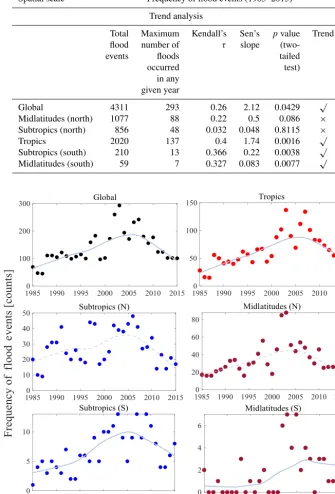
monotonic trends. Figure 2 presents the time series ofFCfor
the global scale and the five latitudinal belts. A solid LOESS (local regression) curve is shown if the trend is significant. Alternately, a dashed LOESS curve is shown for the time series that do not exhibit a statistically significant trend. The detailed statistics derived from the trend analysis are given in Table 2.
A total of 4311 flood events occurred during last 3 decades worldwide. The results of the MK test on the annual fre-quency of global floods indicate that there is a statistically
significant monotonic trend withτ(Kendall correlation
coef-ficient betweenFCand time) andβ(robust Sen slope) values
of 0.26 and 2.12, respectively. A total of 2020 events (out of the 4311 floods) occurred in the tropics. The hypothesis that there is no trend in the frequency of floods in the tropics is rejected. This is also the case for both the subtropics (S) and midlatitudes (S). However, while we see an uptrend in the number of floods in the midlatitudes (S) post-2000, we urge caution in interpreting this trend as zeros dominate the time series. Finally, for both the subtropics (N) and midlati-tudes (N), the hypothesis that there is no trend in the annual frequency of floods cannot be rejected at the 5 % significance level.
– H1. There is a statistically significant increase in the
fre-quency of floods at the global scale, and over the tropics, subtropics (S), and midlatitudes (S). The temporal pat-tern of the data for global floods resembles that of the tropics.
3.2 Addressing H2: trends in the distribution of flood duration
Table 2.Summary of trend analysis (Mann–Kendall test with a significance levelα=0.05) on the frequency of flood events at the global scale and the five latitudinal belts.
Spatial scale Frequency of flood events (1985–2015)
Trend analysis
Total Maximum Kendall’s Sen’s pvalue Trend
flood number of τ slope
(two-events floods tailed
occurred test)
in any given year
Global 4311 293 0.26 2.12 0.0429 √
Midlatitudes (north) 1077 88 0.22 0.5 0.086 ×
Subtropics (north) 856 48 0.032 0.048 0.8115 ×
Tropics 2020 137 0.4 1.74 0.0016 √
Subtropics (south) 210 13 0.366 0.22 0.0038 √
Midlatitudes (south) 59 7 0.327 0.083 0.0077 √
Figure 2.Frequency of flood events at the global scale and the latitudinal scales (i.e., tropics, subtropics – N, subtropics – S, midlatitudes – N, and midlatitudes – S); a LOESS curve fitting is shown (solid line) for the time series in which a significant trend in the number of
flood events is observed (Mann–Kendall test with significance levelα=0.05). A dashed line indicates the LOESS curve for the regions with
insignificant trends.
the flood duration. The following four subsections elaborate the results for each metric.
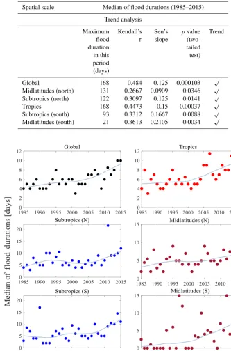
3.2.1 Trends in the median of flood durations
Table 3.Same as Table 2 but for the median of flood durations.
Spatial scale Median of flood durations (1985–2015)
Trend analysis
Maximum Kendall’s Sen’s pvalue Trend
flood τ slope
(two-duration tailed
in this test)
period (days)
Global 168 0.484 0.125 0.000103 √
Midlatitudes (north) 131 0.2667 0.0909 0.0346 √
Subtropics (north) 122 0.3097 0.125 0.0141 √
Tropics 168 0.4473 0.15 0.00037 √
Subtropics (south) 93 0.3312 0.1667 0.0088 √
Midlatitudes (south) 21 0.3613 0.2105 0.0034 √
Figure 3.Same as Fig. 2 but for the median of flood durations.
global scale and all sub-spatial scales. We see that the median of the flood duration at the global scale has increased steadily from 4 days in the year 1985 to 10 days in the year 2015, in-dicating that the median flood duration changed to moderate duration in 2015 from short duration in 1985. In other words, it shifted one class from being less than 1 week to between 1 week and 3 weeks. Similar shifts can be observed in the
Figure 4.Same as Fig. 2 but for median absolute deviation (MAD) of flood durations.
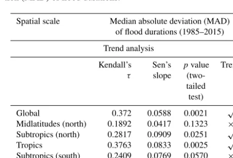
3.2.2 Trends in the median absolute deviation (MAD) of flood durations
The MK trend test is performed on the MAD of flood dura-tion (Eq. 4) at the different global and latitudinal scales and presented in Fig. 4 and Table 4.
The output statistics show that there is a significant in-creasing trend in MAD at the global scale, and in the tropics and subtropics (N). It is interesting to note that the MAD has essentially remained constant, around 2–3 days from 1985 to 2000, and has increased since to around 5 days in 2015, in-dicating increased variability in flood durations within years in these belts recently. There is no significant change in the variability in the midlatitudes (N and S) and subtropics (S).
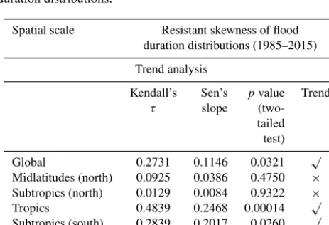
3.2.3 Trends in the resistant skewness of flood duration
The resistant skewness of flood duration is calculated for each time series using Eq. (5) and presented in Fig. 5. As before, the MK trend test is applied to these time series. A statistically significant trend in the skewness is observed at the global scale and tropical and subtropical (S) latitudes. Similar to Tables 2–4, in Table 5 we present the test statis-tics. We observe that the yearly asymmetrical/symmetrical behavior of the distribution of flood durations has
consider-Table 4. Same as Table 2 but for the median absolute devia-tion (MAD) of flood duradevia-tions.
Spatial scale Median absolute deviation (MAD) of flood durations (1985–2015)
Trend analysis
Kendall’s Sen’s pvalue Trend τ slope
(two-tailed test)
Global 0.372 0.0588 0.0021 √ Midlatitudes (north) 0.1892 0.0417 0.1323 × Subtropics (north) 0.2817 0.0909 0.0251 √ Tropics 0.3763 0.0833 0.0025 √ Subtropics (south) 0.2409 0.0769 0.0570 × Midlatitudes (south) 0.1914 0.00001 0.0924 ×
Figure 5.Same as Fig. 2 but for the resistant skewness of flood durations.
Table 5.Same as Table 2 but for the resistant skewness of flood duration distributions.
Spatial scale Resistant skewness of flood duration distributions (1985–2015)
Trend analysis
Kendall’s Sen’s pvalue Trend τ slope
(two-tailed test)
Global 0.2731 0.1146 0.0321 √ Midlatitudes (north) 0.0925 0.0386 0.4750 × Subtropics (north) 0.0129 0.0084 0.9322 × Tropics 0.4839 0.2468 0.00014 √ Subtropics (south) 0.2839 0.2017 0.0260 √ Midlatitudes (south) 0.2903 0 0.0092 √
duration in the subtropics (N) and midlatitudes (N) at the 5 % significance level.
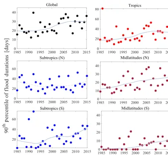
3.2.4 Trends in the 90th percentile of flood durations
Finally, we test for monotonic trend in the extreme values (expressed here as the 90th percentile) of flood duration. This
measure serves as a surrogate for extremely long-duration flood events each year. By definition, the 90th percentile of the flood duration (FDt,r
90) is the value which is exceeded by
only 10 % of the events in that year (year “t”) in the
latitudi-nal belt “r”. Consequently, a value as large as this indicates the long-duration extent of the flood. Figure 6 and Table 6 present the summary of MK analysis on the 90th percentile of flood duration.
The extreme duration of floods has substantially changed over the last 3 decades at the global scale, tropics, midlat-itudes (N and S), and subtropics (S), as presented in Ta-ble 6. The null hypothesis that there is no monotonic trend in the tails is rejected in all regions, except the subtropics (N). Furthermore, we find that the extreme values of the long-duration flood events are more than 30 days in the recent decade, whereas they were less than 20 days in the 1980s and 1990s. The increase was monotonic.
The highlights of trend analyses presented in Figs. 3 to 6 and Tables 3 to 6 are outlined below:
– H2. The median of flood duration has increased at the
in-Figure 6.Same as Fig. 2 but for the 90th percentile of flood durations.
Table 6.Same as Table 2 but for the 90th percentile of flood dura-tion distribudura-tions.
Spatial scale 90th percentile of flood durations (1985–2015)
Trend analysis
Kendall’s Sen’s pvalue Trend τ slope
(two-tailed test)
Global 0.3699 0.4417 0.0037 √ Midlatitudes (north) 0.3355 0.4875 0.0084 √ Subtropics (north) 0.0452 0.0750 0.7338 × Tropics 0.3054 0.6364 0.0165 √ Subtropics (south) 0.2946 0.7385 0.0206 √ Midlatitudes (south) 0.3570 0.3182 0.0038 √
crease in the resistant skewness of flood duration around the globe, tropics, subtropics (S), and midlatitudes (S). For the extreme flood durations (i.e., 90th percentile), we see an increasing trend in all spatial scales except the subtropics (N) over the past 3 decades. Due to the presence of a significant number of zeros in the
statis-tics of the floods, we urge caution in interpreting the trends seen in the midlatitudes (S).
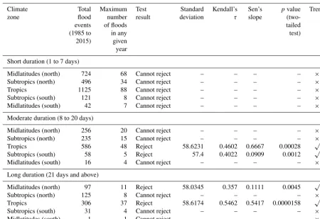
3.3 Addressing H3: trends in the frequency of short-, moderate-, and long-duration floods
Given that we find statistically significant trends in the tails of the distribution (90th percentile of the duration of floods), we were interested in exploring whether there would be a trend in the frequency of the long-duration floods as well. To investigate this, we performed the MK test on the
fre-quency of long-duration floods (FCL) for the tropics,
sub-tropics, and midlatitudes. We also performed these tests on
short-duration flood frequency (FCS) and moderate-duration
flood frequency (FCM). We present these results in Table 7.
Table 7.Summary of trend analysis (Mann–Kendall test with a significance levelα=0.05) on three flood classes: short, moderate, and long durations of flood events over five latitudinal belts.
Climate Total Maximum Test Standard Kendall’s Sen’s pvalue Trend
zone flood number result deviation τ slope
(two-events of floods tailed
(1985 to in any test)
2015) given
year
Short duration (1 to 7 days)
Midlatitudes (north) 724 68 Cannot reject – – – – ×
Subtropics (north) 496 34 Cannot reject – – – – ×
Tropics 1125 88 Cannot reject – – – – ×
Subtropics (south) 121 8 Cannot reject – – – – ×
Midlatitudes (south) 42 7 Cannot reject – – – – ×
Moderate duration (8 to 20 days)
Midlatitudes (north) 256 20 Cannot reject – – – – ×
Subtropics (north) 235 15 Cannot reject – – – – ×
Tropics 586 48 Reject 58.6231 0.4602 0.6667 0.00028 √
Subtropics (south) 58 5 Reject 57.4 0.4022 0.0909 0.0012 √
Midlatitudes (south) 16 4 Cannot reject – – – – ×
Long duration (21 days and above)
Midlatitudes (north) 97 11 Reject 58.0345 0.357 0.1111 0.0045 √
Subtropics (north) 125 8 Cannot reject – – – – ×
Tropics 306 37 Reject 58.6174 0.5462 0.5417 0.0000158 √
Subtropics (south) 31 4 Cannot reject – – – – ×
Midlatitudes (south) 1 1 Cannot reject – – – – ×
results from H2, where we see a trend in the skewness and the tails of floods in these belts. An increase in the frequency of moderate- and long-duration floods will result in a shift of the quantile of flood duration distribution, thereby changing the skewness and the tails.
For the long-duration flood events in the tropics, the total number of events has increased from 60 before 2000 to 249 after 2000. Similarly, the total number of events in the midlat-itudes has increased from 27 to 70 post-2000. In other words, there are 4 times more long-duration floods that occurred dur-ing the most recent 15 years than before the year 2000. The increase across the midlatitudes (N) is around 2.5 times pre-and post-2000.
– H3. In summary, frequency of moderate- and
long-duration flood classes has changed recently, but remains unchanged for the short-duration floods in all the lati-tudinal belts. The annual frequencies of moderate- and long-duration flood events have increased across the tropics and midlatitudes (N) (on the scale of 4 and 2.5 events per year, respectively) over last 3 decades.
3.4 Country-scale vulnerability analysis to short-, moderate-, and long-duration flood events
There were 4311 flood events that occurred from 1985 to 2015 around the world. According to Tables 2 and 7, globally, the total number of short-, moderate-, and
long-duration flood events was 2508 (≈59 %), 1151 (≈27 %), and
560 (≈13 %), respectively. In addition to the aggregate
anal-yses at the latitudinal level, we also explored the country-scale vulnerability to short-, moderate-, and long-duration floods. We interpret vulnerability as the expected value of the damage due to floods, i.e., the severity of the consequence of the floods (Holling, 1978; Hashimoto et al., 1982).
(66 events), Pakistan (66 events), Nigeria (57 events), Malaysia (54 events), Kenya (49 events), Canada (48 events), Colombia (44 events), Peru (43 events), Turkey (41 events), Nepal (40 events), France (40 events), Romania (38 events), Ethiopia (35 events), Somalia (34 events), and New Zealand (31 events).
Then, the fraction of flood frequencies for each country and duration class – short, moderate, and long – is calculated. Figure 7a presents these fractions for the 28 countries using the ternary plot. For 23 of these countries, we have the data on the damages due to the floods. We computed the expected value of the damages for each country and plotted the frac-tional damage due to short-, moderate-, and long-duration floods as the second ternary plot in Fig. 7b. The color bars indicate the total number of events (Fig. 7a) and the total flood damage (Fig. 7b). In each plot, the location of the country shows the relative fraction of short-, moderate-, and long-duration flood frequency and damage. For example, in Fig. 7a, the United States is identified as a red circle in the top
corner with >60 % of floods being short duration, between
20 and 30 % of the floods being moderate, and only<10 %
of them being long-duration floods. However, in terms of the vulnerability to floods (Fig. 7b), the United States is located in the bottom right corner of the triangle, indicating that most of the vulnerability is due to low-probability long-duration floods. Similar observations can be made for Vietnam, Mex-ico, Indonesia, Australia, and Malaysia, to name a few. These countries have a very low probability of long-duration floods, but the consequence of these floods is the most important in terms of the vulnerability. It is also noteworthy to emphasize that for most of the countries, the overall damage is dom-inated by the damage due to moderate- and long-duration floods. This can be seen from the fact that many of the coun-tries are found in the bottom left and right corners of the ternary plot.
To further understand the relation between flood duration and flood damage, we fit log-linear models given in Eq. 6 for four selected countries: the United States, Thailand, In-dia, and China. The results of the log-linear models for these four countries are shown in Fig. 8a. These countries are se-lected because they have the highest number of long-duration
floods among all countries (Fig. 8b). Parameterβis the
scal-ing exponent of the damages to the flood duration. Note that the scaling exponent is similar for the United States (0.89) and China (1.03) while India (0.23) and Thailand (0.56) have much smaller exponents. In total, 226 flood events occurred across India, of which around 43, 32, and 25 % of them were short-, moderate-, and long-duration events, respectively. In the United States, short-, moderate-, and long-duration flood events account for 66, 26, and 8 % of 388 flood events that occurred in the last 3 decades. However, the fraction of long-duration flood events is much higher for Thailand (30 % of total flood events). In China, around half of the flood events were related to the moderate- or long-duration flood classes (34 and 16 %, respectively). This opens up new questions
about whether there are consistent relations like this across the globe and how different these scaling exponents would be. We do not pursue them as part of this investigation, how-ever, in the spirit of examining flood duration and damages, in Fig. 8b and c, we present the data on flood duration and flood damage ranked for various other countries.
According to the DFO flood data from 1985 to 2015, the ranking results show that the frequency of short-duration floods for the United States, China, India, and the Philippines is respectively 255, 173, 133, and 122. For moderate-duration floods, the countries of China, the United States, India, and the Philippines have experienced 118, 101, 74, and 52 flood events, respectively. The long duration floods were seen mostly in India (55 events), China (53 events), the United States (32 events), and Thailand (20 events) from 1985 to the end of 2015. It should be noted that here we only presented the top 21 countries in each category.
As discussed in this section, the consequences of floods of different durations should be paid attention to, as this plays a big role in designing appropriate flood-proofing infrastruc-ture and developing early warning systems and flood insur-ance payout structures. The relation between the duration of floods and the induced damages, and how they might vary across different countries, was also investigated here.
4 Discussion
The trends in the frequency and the distribution of the floods (prominent in long-duration floods) may be related to several causes ranging from measurement uncertainty in the DFO flood data, climate and atmospheric teleconnections, and so-cioeconomic contributions such as the increased exposure to the flood events. We attempt to explain these possibilities in the following two sections.
4.1 What are the uncertainties in DFO flood archive data, and/or has the exposure to the flood events changed?
Total flood events
(b)
(a)
Total flood damages
[log10 USD]
-Figure 7.(a)Relative frequency of short- (less than 7 days), moderate- (8 to 20 days), and long-duration (21 days and above) floods for
the countries with at least 31 events from 1985 to 2015;(b)relative flood damages due to short-, moderate-, and long-duration floods with
0 50 100 150 200 250 USA China Indonesia Philippines India Australia Iran Vietnam Afghanistan Japan Mexico Brazil Russia Pakistan SouthAfrica Bangladesh UK Nigeria Turkey Canada France
Total number of short-duration floods
[1985 – 2015]
0 50 100
China USA India Philippines Indonesia Australia Vietnam Bangladesh Brazil Mexico Thailand SriLanka Russia Malaysia Afghanistan Ethiopia Nigeria Iran Romania Canada Kenya
Total number of moderate-duration floods
[1985 – 2015]
0 10 20 30 40 50 60
India China USA Thailand Australia Brazil Kenya Pakistan Colombia Bangladesh Indonesia Chad Vietnam Argentina Mozambique Nepal Peru Sudan Malaysia Paraguay Russia
Total number of long-duration floods
[1985 – 2015]
1 10 100 1000
USA Canada China UK Iran South Korea India Turkey Venezuela Philippines Taiwan Thailand Australia Indonesia France Austria Fiji North Korea Argentina South Africa Switzerland Millions
Total damages due to short-duration floods
[1985 – 2015]
1 10 100 1000 10 000
China Romania USA India Philippines UK France Taiwan Italy Bangladesh Mexico Brazil Pakistan Bolivia Iran Russia Argentina Germany Vietnam Indonesia Thailand Millions
Total damages due to moderate-duration floods
[1985 – 2015]
1 10 100 1000 10 000
China USA Germany North Korea India Mexico Argentina Vietnam Bangladesh Mozambique Australia Indonesia Namibia Peru Guyana Thailand Malaysia Canada South Africa Pakistan Sudan Millions
Total damages due to long-duration floods
[1985 – 2015]
[USD ($), log-scale] (c)
(b)
(a)
D
[Counts]
Figure 8.(a)Covariation of flood duration with the corresponding flood damages for the top four countries with the maximum number
of long-duration flood events (i.e., India, China, the United States, and Thailand),(b)total number of short- (less than 7 days),
moderate-(8 to 20 days), and long-duration (21 days and above) floods, and(c)total damages due to short-, moderate-, and long-duration floods. These
clouds, cloud shadows, and mountainous terrain (Braken-ridge et al., 1998). Further, inclusion of this improved tech-nology will result in better monitoring of floods. This im-provement is likely a potential driver of trend in the flood duration. In our analysis of H3, we find that there is no sig-nificant trend in the frequency of short-duration events across all latitudinal scales (Table 7), but a significant trend can be seen across the tropics for moderate- and long-duration flood events. The introduction of improved satellite products would have increased the chances of detecting more short-duration floods (small events) along with providing better resolution for longer floods. We think that it is not possible to see the systematic contributions of such products into only one specified type(s) of flood duration.
To validate the DFO’s flood statistics, we have corrobo-rated the DFO floods with the available in situ streamflow ob-servations from the GRDC (The Global Runoff Data Centre, 56068 Koblenz, Germany, 2013, http://grdc.bafg.de, last ac-cess: 1 December 2017). Among the stations that had match-ing time periods and locations, we found that a high percent
of stations (≈90 %) have very few errors (i.e., less than 7
days) when their flood durations were compared. The re-sults demonstrate that the recorded flood information in the DFO appears to be reliable with respect to the GRDC river discharge measurements (see more details in Appendix B). However, we did identify a reporting bias in the start and end dates of the floods where the events with no reported flood beginning date are assumed to start in the middle of the month. Some biases were also identified for days 1, 5, 10, 15, 20, and 25, which had an increased number of flood counts. These biases will potentially lead to estimation un-certainties in the trend model. We believe that interpretation at the global level will remain robust due to the effect of av-eraging and large numbers; at the local level interpretation needs more attention to such reporting details.
While understanding such uncertainties is essential, espe-cially while interpreting trends in limited data, it is also doc-umented in the literature that there has been an increased ex-posure to floods in recent times. The number of people, res-idential and industrial properties, and assets exposed to the flood events has drastically increased (Bouwer, 2011; Jong-man et al., 2012; Kundzewicz et al., 2014). The type of vul-nerability to flood risk is mostly connected to development of the country and its land use and environmental manage-ment (Peduzzi et al., 2009). Recent studies by Di Baldassarre et al. (2010) and Vogel et al. (2011) in Africa and the United States, respectively, showed that there had been a consider-able change in the flood frequency and magnitude in regions which have undergone intense urbanization.
While exposure of people to floods is the main concern in developing countries, exposure of assets and properties to floods is the vital concern for the developed countries (Jong-man et al., 2012). Recently, much residential and industrial infrastructure has moved to the flat and cheap lands of flood-plains (Peduzzi et al., 2011). The nature of
geomorphologi-cal features of land has been modified to embrace these new developments. Hirabayashi et al. (2013) and Stevens et al. (2016) have recently indicated that the increase in the report-ing of floods can be linked to the rise in the land use devel-opment in the floodplains.
4.2 Can the trends be related to natural variability in the climate and atmospheric systems?
The frequency of heavy precipitation events has increased at the global scale (Groisman et al., 2005; Zhou et al., 2013; Liu and Zipser, 2015). Using daily precipitation observations from the Global Historical Climatology Network (GHCN) dataset, Alexander et al. (2006) showed that the distribu-tions of precipitation indices in the 1979–2003 period are significantly different from the 1901–1950 period with a ten-dency towards wetter conditions. Solomon (2007), in the fourth assessment report of the Intergovernmental Panel on Climate Change (IPCC), discussed that the annual precip-itation intensity has increased over high latitudes during the period from 1901 to 2005, except the southwest of the United States, northwestern Mexico, and the Baja California Penin-sula. This IPCC report also highlights the increasing con-tribution of extreme rainfall events to the total precipitation across Europe and the United States, which mostly occurred during the last 3 decades of the 20th century. Westra et al. (2013) tested 8326 land-based rainfall stations (with at least 30 years of record from 1900 to 2009) and found that the an-nual maximum daily precipitation has significantly increased for more than two-thirds of these stations at the global scale. Theoretical studies also discussed the fact that mean global precipitation intensity increased by 1–3 % (conditional on
available energy budgets) in proportion to the 1◦C increasing
rate of surface air temperature. Trenberth (1999), Trenberth et al. (2003), Trenberth (2011), Schiermeier (2011), and Glur et al. (2013) among others have also argued that an in-crease in air temperature will inin-crease the atmospheric water-holding capacity (Clausius–Clapyron relationship), leading to more intense and frequent precipitation events. Hence, fluctuating precipitation regimes would interrupt the current balances of components within the hydrological cycle and human activities (Doherty et al., 2000; Dentener et al., 2006). Consequently, a warmer and wetter atmosphere is likely to intensify the global water cycle that ultimately will result in more frequent and larger flood events.
Hence, in an effort to investigate any significant relation-ship between the observed trend in the flood data (charac-terized in H1 and H2) and the variability in the climate and atmospheric circulation patterns, we considered large-scale atmospheric teleconnections and climate indices (with quasi-periodicity in nature that can lead to wet–dry regimes) to ex-plain the trend, i.e., to place the short-term trends within a longer climate variability context as argued by Merz et al. (2012) and Armal et al. (2017).
Addressing H4: relationship between observed trend(s) in hypotheses H1 and/or H2 and the atmospheric
teleconnections
Our hypothesis (i.e., H4) is that the detected time trend is due to cyclical climate influences (i.e., oscillatory behavior) asso-ciated with the large-scale ocean–atmospheric interactions as recorded in the ENSO, AMO, PDO, and NAO indices. The corresponding residual time-trend analysis from the models explains whether the long-term natural variability dominates the trends. We considered Poisson distribution as the link
function forFCandFD90andFDMedianin the GLM framework
since they represent the counts. The detailed information on the GLM’s outputs, best-choice explanatory variables, and the MK test’s outputs on the residuals is shown in Table 8. The most important remarks from Table 8 are given below.
1. ENSO, AMO, and NAO are related toFCat the global
scale. There is no statistically significant trend in the residuals of the model, indicating that the trend initially observed in the global flood frequency data could be in part due to the variability in these indices. AMO and PDO in the tropics, AMO in the subtropics, and AMO and PDO in the midlatitudes (S) are the climate indi-cators that are dominant in explaining the variability in the flood frequency. The trend in the residuals is nonex-istent. Together, we can see that the monotonic trend ini-tially observed in the frequency of floods at the global and the sub-spatial scales may be due to the variability in the climate and atmospheric teleconnections. Ward et al. (2016) and Emerton et al. (2017) have previously demonstrated the role of ENSO in modulating global floods. In addition, Hodgkins et al. (2017) demonstrated recently that AMO has a significant negative (positive) relationship with 25- and 50-year flood occurrence for large (medium) catchments in North America (Europe). Our results corroborate with their remarks along with showing that the decadal oscillations also modulates the floods both at the global scale and in each latitudinal belt.
2. We did not find any significant climate indicators that can explain the variability in the median of the floods except for the midlatitudes (S). However, as we pointed out before, given the limited data available at this lat-itudinal belt, we do not further interpret these climate
indicators as causing the trends. There should be one or a set of inexplicable factor(s) beyond climate
telecon-nections that might drive the observed trend inFDMedian.
We speculate that this increase relates to improved in-strumentations and LULC conditions among others.
3. AMO and NAO have an association withFD90 at the
global scale. There is no statistically significant trend in the residuals after adjusting for the background vari-ance. In the midlatitudes (N), the trends in the extreme
flood duration values (i.e.,FD90) can be explained using
AMO, PDO, and NAO. In the tropics, AMO, PDO, and
NAO are related to theFD90, but we still observe a
sta-tistically significant trend after adjusting for this factor.
In contrast, the trend inFD90 across the subtropics (S)
can be related to ENSO, AMO, and NAO. ENSO and NAO can explain the trends across the midlatitudes (S).
– H4. In summary, we have approached the explanation of
observed trends in an exploratory spirit and formulated models based on well-known atmospheric teleconnec-tions. We see that the observed trends in flood frequency across the globe and tropics can be largely linked to the decadal and multidecadal climate variability. Regarding the flood duration, the observed trends in the median could not be associated with any of these climate fac-tors, while extreme flood duration can be partially asso-ciated with AMO for the globe and tropics and ENSO for the southern subtropics and midlatitudes. We note that the time series (both observed variables and ex-ogenous variables) may have autocorrelation structure that may manifest as a trend in limited data. Detection of autocorrelation before ascribing trends is important. We investigated for any structured autocorrelation in the residuals after accounting for the exogenous variables and found none. We did not examine the effect of the lagged dependence of the climate variables here. One can develop models in which an appropriate lag can be chosen based on the model performance.
4.3 Comparison of results to recent studies
To our knowledge, this study is the first analysis of global flood events that exclusively focuses on the variability in the flood duration using the DFO dataset over the last 3 decades (i.e., 1985–2015). In this part, we are corrobo-rating the presented results here with the most relevant previous studies. A high number of recent flood stud-ies have focused on the regional scale, and/or have used the flood duration to calculate the flood magnitude (i.e.,
log×duration×severity×affected area). For instance,
b) that there is an increasing tendency in the number of floods with large magnitude and severity in Europe. These are con-sistent with our findings.
Several flood-related studies analyzed the trends in the an-nual maximum streamflow and/or precipitation across multi-ple spatiotemporal scales. For exammulti-ple, an increasing trend in annual maximum precipitation intensities was found by Min et al. (2011) in addition to the increasing trend in the ex-treme precipitation (Lehmann et al., 2015) at the global scale, but the catchment characteristics and river geomorphology can substantially regulate the streamflow regimes despite the intensified rainfall trends (Hall et al., 2014). Recently, Do et al. (2017) used the Global Runoff Data Center (GRDC) database to investigate the potential trends in the annual max-imum streamflow and found decreasing trends for many sta-tions in western North America but increasing trends in east-ern North America, some parts of Europe and South Amer-ica, and southern Africa. A complete comparative analysis is required in this regard, especially to identify the DFO lo-cations with the river basins and then analyze the trends in those river basins. We believe that this involves developing a separate study in the future.
5 Conclusions
A global assessment of flood events is performed here, fo-cusing on the flood frequencies and duration characteris-tics at different global–latitudinal–country scales from the year 1985 to 2015. The comprehensive assessment of the fre-quencies of flood events and characteristics of the probability distribution of flood durations presented here is the very first large-scale study of “actual” flood events worldwide focus-ing on understandfocus-ing the temporal changes over the last 3 decades. It was verified here that the frequency of floods in-creased at the global scale, tropics, subtropics (S), and mid-latitudes (S). Selected metrics of the flood duration showed a monotonic increasing trend for the median (at all spatial scales), MAD (across the globe, tropics, and subtropics – N), resistant skewness (across the globe, tropics, subtropics – S, and midlatitudes – S), and extremes (all spatial scales except the subtropics – N). More importantly, we find that the fre-quency of moderate- and long-duration floods has increased recently, but remains unchanged for the short-duration floods at all spatial scales. The trends in the flood frequency and ex-treme durations at a global scale can be largely ascribed to ENSO, AMO, and NAO, the interannual to decadal to mul-tidecadal modes of variability, while the trend in the median flood durations remains unexplained. An overall summary is presented below.
– The frequency of flood events has increased; the
year 2003 is recognized as the year with the maximum number of flood occurrences across all spatial scales; however much of this increase is within the long-term decadal to bi-decadal climate cycles.
– There is a statistically significant trend in the moments
of the flood duration at the global scale, tropics, sub-tropics, and midlatitudes; the extreme floods post-2000 are more than 30 days as opposed to less than 20 days in the 1980s and 1990s. These trends in extreme flood
du-rations (FD90) can be related to climate teleconnections,
whilst the trend in the median is still unexplained.
– The yearly number of moderate- and long-duration
flood occurrences increased (from before to after the 2000s) by a factor of 4 and 2.5 events per year across the tropics and midlatitudes (N), respectively.
– There was no monotonic trend observed in the
frequen-cies of short-duration floods (i.e., flood duration of 1 to 7 days) across all the spatial scales.
– Comparison of the DFO flood events with the
corre-sponding GRDC streamflow over the midlatitudes (N) and subtropics (N) (locations that had common records) reveals that the reported flood events by the DFO are reasonably reliable. For instance, 90 % of the events contain less than 7 days of deviation in their flood dura-tions.
In addition, we also presented a simple overview of the vulnerability profile for different countries. This can be help-ful to inform and improve the flood warning systems tailored to the various types and resource management practices dur-ing the post-disaster responses. Furthermore, with increas-ing globalization, countries are now interdependent through supply chain networks to achieve streamlined production and overall cost reductions. A country-level understanding of the exposure to different types of floods can help more accurately predict the vulnerable nodes that might cause a systemic net-work failure. It can also provide the necessary analysis for pricing and portfolio risk management for the agencies that insure and hedge against the flood losses.
While this study explores the trends in the frequency and duration of global floods, especially the long-duration floods, it is necessary to investigate the cause–effect mechanism of these trends along with socioeconomic variables to fully un-derstand the emergence of floods. Unun-derstanding these hier-archical layers will provide us with comprehensive informa-tion and realizainforma-tion that can be translated into better defining the multiscale flood risk management and damage control strategies.
Appendix A: Nonparametric trend test
The nonparametric rank-based Mann–Kendall (MK) test is widely applied to detect the monotonic trend (i.e., a grad-ual change over time with consistency in direction) in cli-matic or environmental time series (Mann, 1945; Kendall, 1948). It is an appropriate approach to be employed for the type of variables that exhibit skewness around the general relationship (Helsel and Hirsch, 1992). The MK’s
null hypothesis (H0) is that there is no monotonic trend
(i.e.,−Z1−α
2 ≤ZMK≤Z1− α
2) (Hirsch, 1992). A failure to
re-jectH0indicates that the data are not sufficient to conclude
that a trend might be existing, bounded to that specified level of confidence (Meals et al., 2011). The MK test is based on
theSstatistic as the sum of integers given in the form
S=
T−1
X
p=1 T
X
q=p+1
Sign yq−yp,where Sign yq−yp
=
+1 if yq−yp
>0
0 if yq−yp=0
−1 if yq−yp<0
. (A1)
Also,
ZMK=
S−1
√
Var(S) ifS >0
0 ifS=0
S+1
√
Var(S) ifS <0
, (A2)
whereT is the total number of observations andyqandypare
the data values in the time series p andq (p > q),
respec-tively. Hence, three cases can be associated with theSvalue
derived from Eq. (A1) (Helsel and Hirsch, 1992) as
1. it is a large positive number: an upward trend is ob-served since the later-measured values tend to be larger than earlier ones;
2. it is a large negative number: a downward trend is indi-cated since the later values tend to be smaller than ear-lier ones;
3. it is an absolute small number: no trend is indicated.
Further, the Kendall’s tau (τ) nonparametric correlation
coefficient and Sen’s slope (β) (i.e., rate of consistent
change) (Sen, 1968) can be computed as
τ = S
T(T−1) 2
; andβ=median
yq−yp
xq−xp
,
p=1,2, . . ., T−1 andq=2,3, . . ., T (A3)
where Kendall’s tau (τ) value is between−1 and+1 (similar
to correlation coefficient in linear regression analysis).
Table B1.Summary of GRDC stations (<110 km) with available daily observations (at least) from 1985 to 2015 adjacent to the cor-responding reported DFO flood events.
Spatial scale Number of Average Average
adjacent distance length of
GRDC to GRDC available
stations station daily
with data (km) observations
(years)
Global 517 54.95 72.78
Midlatitude (north) 319 44.86 80.13
Subtropics (north) 122 49.3 85.43
Tropics 12 34.22 60.92
Subtropics (south) 62 41.85 58.45
Midlatitude (south) 2 104.53 79
Appendix B: Comparing the DFO’s flood database with the GRDC and EM-DAT databases
B1 Validating the DFO’s flood duration using the GRDC river discharge measurements
We validated the reported flood statistics in the DFO database with in situ discharge observations from the Global Runoff Database from GRDC (the Global Runoff Data Centre, 56068 Koblenz, Germany, 2013, http://grdc.bafg.de). The GRDC global-scale streamflow dataset maintains records of more than 9000 stations with an average available length of 42 years per station. From the 4311 DFO global flood events, we found 517 stations in the GRDC database that have a tem-poral span matching 1985–2015 and are within a radial
dis-tance of 110 km (≈1◦radial distance). Among these stations,
319 are found in the midlatitudes (N) and 122 are found in the subtropics (N). Further, these stations are predominantly located in the United States, Europe, and South Africa. A summary of the identified GRDC stations in this validation across different spatial scales is presented in Table B1.
We employed the following procedure to validate this common record.
1. Three flow exceedance thresholds (Q∗) as the 90th,
95th, and 99th percentile of the entire daily stream-flow time series are calculated for each station sepa-rately. These thresholds for flood definition are consis-tent with earlier studies on this subject (e.g., Wu et al., 2012, 2014; Koirala et al., 2014; Asadieh and Krakauer, 2017).
3. Then, the total number of day(s) within the DFO’s flood span when the daily streamflow exceeds the
thresh-old (Q∗) is recorded as the GRDC’s flood duration.
4. The difference between these two estimates is calcu-lated asFD{DFO}−FD{GRDC}.
If the GRDC flood duration is as long as the flood dura-tion of the DFO, we consider this to be a perfect match and the difference is 0. If GRDC did not exhibit a threshold ex-ceedance flow during the DFO span, we consider this to be a miss and the difference will be as high as the flood dura-tion for the DFO. Hence the absolute error is between 0 and
FD{DFO}. We group this error into four categories: 0, [1–7], [8– 20), and 21 days and above for each spatial unit. The results are presented in Table B2.
At the global scale and over the midlatitudes (N), for a threshold of the 90th percentile, up to 90 % of the events have an error of less than 7 days, indicating that the GRDC stations had experienced threshold exceedance floods when the DFO reported a flood. Even if we increase the threshold to the 95th percentile, we still have up to 85 % of the events with a de-viation of less than 7 days. A similar pattern is seen for the subtropics (N). We refrain from interpreting the error results for the other spatial units as most of the GRDC matching data are only found in the midlatitudes (N) and subtropics (N).
Despite certain uncertainties in calculating flood duration (such as the distance between the GRDC station and the lo-cation of a flood event, anthropogenic inputs to the nature of flow rates, and a physical streamflow exceeding thresh-old that could precisely mimic the occurrence of a realistic flood event), it can be concluded that around 80 % of GRDC stations in this comparison could verify that the recorded flood information in the DFO including the start–end dates and flood duration parameters is reliable and would pro-vide a certain path towards assessment of global flood events since 1985.
B2 Comparing the DFO’s flood frequency with the EM-DAT database
We corroborated the global DFO’s flood frequency with the flood frequency data available at global scale from the EM-DAT database (the Emergency Events Database, http: //www.emdat.be/database) during the same time frame (1985 to 2015). As presented in Fig. B1, we can see that the origi-nal EM-DAT flood frequency time series (which is based on the reporting information) compares well with the DFO data (which are based on both satellite observations and report-ing information). It should be noted that for a disaster to be recorded in the EM-DAT database, at least one of the follow-ing criteria must be satisfied: (1) 10 or more people reported killed, (2) 100 or more people reported affected, (3) there was the declaration of a state of emergency, and (4) there was a call for international assistance. We see a similar trend in EM-DAT data as in the DFO data, indicating a potential
increase in floods due to various causes. It can be also in-ferred that the DFO is collecting more flood information, especially those events that occur in the regions with zero access to reporting facilities. The Pearson correlation coef-ficient between these two flood frequency datasets is 0.636
with apvalue=0.0001 (it is significant at the 5 %
signifi-cance level).
B3 Distribution of start and end dates of the DFO flood events within a month
We investigated the DFO-reported flood events from 1985 to 2015 in terms of the distribution of the flood beginning date and flood end date within each month. For the start-ing date of flood, there are less than 5 % (194 events) out of 4311 events that have been reported with the flood begin-ning date as the middle of the month. There are 282 events reported on the first day of the month. Together, the first and the middle day of the month account for a total of 476 out
of 4311 events (≈11 %). Furthermore, days 1, 5, 10, 15,
20, and 25 also have an increased number of flood counts
(≈4 %), suggesting a reporting bias (likely rounding off of
Figure B1.Frequency of flood events from the DFO database and EM-DAT at the global scale (1985–2015).
(a) (b)
Counts
Day in month Day in month
Table B2.Comparing flood duration (FD) reported by the DFO and calculated from the GRDC ground-based observations for the global
scale and over five latitudinal belts. Three flood-related exceeding thresholds (i.e., 90th, 95th, and 99th) are derived from the entire daily observations of the GRDC stations located adjacent to the centroid of the flood event reported by the DFO.
Spatial scale FD{DFO}−FD{GRDC}(days)
0 [1–7] [8–20] >20 0 [1–7] [8–20] >20 0 [1–7] [8–20] >20
No. of counts(inside parentheses as %)
GRDC flood threshold 90th percentile 95th percentile 99th percentile