https://doi.org/10.5194/npg-26-291-2019 © Author(s) 2019. This work is distributed under the Creative Commons Attribution 4.0 License.
Mahalanobis distance-based recognition of changes
in the dynamics of a seismic process
Teimuraz Matcharashvili1, Zbigniew Czechowski2, and Natalia Zhukova1 1M. Nodia Institute of Geophysics, Tbilisi State University, Tbilisi, Georgia 2Institute of Geophysics, Polish Academy of Sciences, Warsaw, Poland Correspondence:Teimuraz Matcharashvili ([email protected]) Received: 23 December 2018 – Discussion started: 5 February 2019
Revised: 17 July 2019 – Accepted: 26 July 2019 – Published: 27 August 2019
Abstract. In the present work, we aim to analyse the regu-larity of a seismic process based on its spatial, temporal, and energetic characteristics. Increments of cumulative times, in-crements of cumulative distances, and inin-crements of cumula-tive seismic energies are calculated from an earthquake cata-logue for southern California from 1975 to 2017.
As the method of analysis, we use the multivariate Maha-lanobis distance calculation, combined with a surrogate data testing procedure that is often used for the testing of non-linear structures in complex data sets. Before analysing the dynamical features of the seismic process, we tested the used approach for two different 3-D models in which the dynam-ical features were changed from more regular to more ran-domised conditions by adding a certain degree of noise.
An analysis of the variability in the extent of regularity of the seismic process was carried out for different complete-ness magnitude thresholds.
The results of our analysis show that in about a third of all the 50-data windows the original seismic process was in-distinguishable from a random process based on its features of temporal, spatial, and energetic variability. It was shown that prior to the occurrence of strong earthquakes, mostly in periods of generation of relatively small earthquakes, the per-centage of windows in which the seismic process is indistin-guishable from a random process increases (to 60 %–80 %). During periods of aftershock activity, the process of small earthquake generation became regular in all of the windows considered, and thus was markedly different from the ran-domised catalogues.
In some periods within the catalogue, the seismic process appeared to be closer to randomness, while in other cases it became closer to a regular behaviour. More specifically, in
periods of relatively decreased earthquake generation activity (with low energy release), the seismic process appears to be random, while during periods of occurrence of strong events, followed by series of aftershocks, significant deviation from randomness is shown, i.e. the extent of regularity markedly increases. The period for which such deviation from random behaviour lasts depends on the amount of seismic energy re-leased by the strong earthquake.
1 Introduction
The process of earthquake generation remains a focus of diverse interdisciplinary investigations by Earth science re-searchers worldwide. The practical and scientific reasons for this interest are well known and easily explainable. However, despite this strong interest and the enormous research efforts that have already been applied, many important aspects of the complex seismic process characterised by space and time clustering are still not clear (Bowman and Sammis, 2004; Godano and Tramelli, 2016; Kossobokov and Nekrasova, 2017; Matcharashvili et al., 2018; Pasten et al., 2018).
Kossobokov and Nekrasova, 2017). Moreover, the results of analyses carried out to assess the dynamical features of the seismic process in terms of its separate domains (time, space, and energy) also indicate differences in behaviour (see e.g. Goltz, 1998; Matcharashvili et al., 2000, 2002; Abe and Suzuki, 2004; Chelidze and Matcharashvili, 2007; Iliopou-los et al., 2012). More specifically, it has been shown that the seismic process in the temporal and spatial domains may reveal features that are close to so-called low-dimensional dynamical structures, although the features of the behaviour in the energy domain appear close to randomness, i.e. repre-senting high-dimensional dynamical processes (Goltz, 1998; Matcharashvili et al., 2000; Iliopoulos et al., 2012). This has been shown for whole catalogues as well as for their parts and for different time periods.
Coming back to the concept of a critical state, it should be emphasised that intermittent criticality implies time-dependent variations in the activity during a seismic cycle. Thus, since the critical state is usually described as the state of the system when it is at the boundary between order and disorder (Bowman et al., 1998), we can describe the time variability of the seismic process in terms of the contempo-rary concept of geocomplexity (Rundle et al., 2000).
According to present knowledge, and in complete accor-dance with the concept of intermittent criticality, it is ac-cepted that the extent of regularity (order) of the seismic pro-cess may vary in all its domains (temporal, spatial, and en-ergetic) (Goltz, 1998; Abe and Suzuki, 2004; Chelidze and Matcharashvili, 2007; Iliopoulos et al., 2012; Matcharashvili et al., 2000, 2002, 2018). At the same time, despite the large number of recent publications demonstrating the diversity of these changes in the dynamics of the seismic process, inter-est in this issue continues to grow. In this context, it should be emphasised that it is important to assess these dynamical changes on the basis of multivariate analysis, taking into ac-count all the temporal, spatial, and energetic constituents of the seismic process. Thus, one important research task is to understand the character of these changes in the entire seis-mic process.
Based on the state-of-the-art studies mentioned above, we aim in the present work to investigate the dynamical features of the seismic process based on all its temporal, spatial, and energetic characteristics. We carry out a multivariate com-parison of the seismic process using an original earthquake catalogue for southern California and a set of randomised
Figure 1.Map of the area covered by the southern California earth-quake catalogue (1975–2017).
catalogues in which unique (temporal, spatial, and energetic) dynamical structures have been intentionally distorted by a shuffling procedure. This multivariate comparison of an orig-inal catalogue with randomised catalogues may help us to gain new knowledge about the character of the changes that occur in the extent of order/disorder of the seismic process. In addition, we will have stronger arguments regarding where and how the dynamics of the original seismic process in the analysed catalogue was close to disorder (irregularity) or order (regularity). We also aim to determine whether such changes are related to the process of preparation for strong earthquakes.
The results obtained in our research show that the extent of regularity in the analysed seismic process changes and is closer to randomness in the periods prior to strong earth-quakes. After strong earthquakes, the regularity of the orig-inal seismic process assessed based on its temporal, spatial, and energetic characteristics is clearly increased.
2 Data used
We based our analysis on the southern California (SC) earthquake catalogue, which is available from http://www. isc.ac.uk/iscbulletin/search/catalogue/ (last access: Novem-ber 2018). We focused on the time period from 1975 to 2017 (see Fig. 1). According to results of a time completeness analysis, the SC earthquake catalogue for the considered pe-riod is complete forM=2.6.
earth-quake catalogue used here. This approach was based on a widely accepted practice (see e.g. Bak et al., 2002; Chris-tensen et al., 2002; Corral, 2004; Davidsen and Goltz, 2004; Matcharashvili et al., 2018) in which all events are assumed to be on the same footing and the catalogue is considered as a whole. In other words, we did not pay attention to the details of tectonic features, the locations of the earthquakes, or their classification as mainshock or aftershock (Bak et al., 2002; Christensen et al., 2002; Corral, 2004).
3 Methods of analysis
In view of our research goal, i.e. a multivariate assessment of the extent of the regularity of the original seismic process, we need to analyse the seismic process in terms of the si-multaneous variability in all three of its domains: temporal, spatial, and energetic. From this point of view, we consider cumulative sums of the characteristics of earthquakes in the temporal, spatial, and energetic domains (Fig. 2). The cumu-lative sum representation in the time domain is trivial, since time is already a cumulative characteristic, representing the cumulative sum of inter-earthquake times. Cumulative repre-sentation in the spatial domain is also quite feasible, and we consider cumulative sums of distances between consecutive earthquakes in the seismic catalogue. The cumulative sum of seismic energies released by consecutive earthquakes is also often used in the context of the different aspects of earth-quake generation (e.g. Bowman et al, 1998; Bowman and Sammis, 2004; Nakamichi et al., 2018). Here, we add that despite some controversies (see e.g. Corral, 2004, 2008) over the question of the reliable energetic measurement of earth-quake size, its relation to the magnitude of an earthearth-quake is generally accepted. Thus, from the earthquake magnitudes in the SC catalogue, we can calculate the amount of seismic energy released, according to Kanamori (1977).
We start from the first earthquake in the catalogue (for the time period of interest, from 1975 to 2017), which we consider a starting point, and then follow the time sequence. Thus, ICT(i) is theith interevent time (i.e. the time between theith earthquake and the (i-1)th earthquake); ICD(i) is the distance between consecutive events and ICE(i) is the energy of the ith earthquake. We can also define these quantities in terms of increments of the cumulative sums; i.e. ICT(i), ICD(i), and ICE(i) are the increments of cumulative sums of the interevent times, interevent distances, and seismic energy released by consecutive earthquakes, respectively.
In order to have the same standard deviation for the three groups of data, the standard deviations were calculated for each of the ICT(i), ICD(i), and ICE(i) data sets, and the data sets were then normalised to have their standard deviations equal to 1.
In order to characterise the seismic process from a multi-variate point of view, we used a well-known statistical test, the Mahalanobis distance (MD) calculation. Calculation of
the MD is an effective multivariate method for different clas-sification purposes and is often used for data sets of different origins. Thus, the objective of our analysis can be regarded as a classification task of the features of a seismic process, assessed using the variability in ICT(i), ICD(i), and ICE(i).
In other words, we aimed to assess the changes that oc-curred in the seismic process over the period covered by the SC catalogue (1975–2017). It is well known that the cor-rectness of a multivariate assessment and classification of a system is strongly dependent on correct feature extraction (McLachlan, 1992, 1999). In other words, the data sets used should be specifically focused on the targeted features of the process under investigation. Hence, in order to have data sets with a similar physical sense, enabling us to assess the dynamical features of seismicity in three domains, we used ICT(i), ICD(i), and ICE(i) data sets.
The MD (Mahalanobis, 1930; McLachlan, 1992, 1999) is a widely accepted method of measuring the separation of two groups of vectors (e.g. one group A, consisting ofNAvectors ai=(aix, aiy, aiz), and another group B, with NB vectors bi). In this method, the difference between the groups can
be considered in terms of the difference between the mean vectorshaiiandhbiiof each group relative to the common
within-group variation. This allows us to draw a conclusion on whether the investigated groups are similar or dissimilar. The MD (often denoted asD) can be calculated from the fol-lowing expression:
D2=(haii − hbii)TS−1 (haii − hbii) , (1)
whereSis the pooled covariance matrix S=(NA−1)SA+(NB−1)SB
NA+NB−2
, (2)
and SA, SB are covariance matrices of the corresponding groups, e.g.
SA= 1 NAX
T
AXA. (3)
The superscripts “T” and “−1” denote the transpose and the inverse operators, respectively. The rows of matrixXA(XB) form the components of theNA(NB) vectorsai(bi), e.g.
XA=
a1x a1y a1z
. . . . . . . . . . . . . . . . . . aNAx aNAy aNAz
. (4)
In general, two conditions or states of a system are more likely to fall into the same class or group (or have a higher probability of being similar) if the calculated MD value is smaller. In order to assess the significance of the difference between the groups, Hotelling’sT2statistic was used, con-verted into an F value and assessed using an F test. The F value was calculated as follows:
F = NANB(NA+NB−p−1)
(NA+NB)(NA+NB−2)p
Figure 2.Cumulative sums of(a)interevent times;(b)inter-earthquake distances; and(c)released seismic energies, starting from the first event in the southern California catalogue (1975–2017).
In Eq. (5),pis the degrees of freedom. Then, in order to draw a final conclusion on the similarity or dissimilarity of the two groups, we compare the calculated F values with a critical value Fc (corresponding to the degrees of freedom). In the case whereF > Fc, a statistically significant difference be-tween the groups is established, with a specific probability (significance level).
When dealing with analysis of complex seismic processes, it needs to be pointed out that the MD calculation is sensi-tive to inter-variable changes in a multivariate system (Ma-halanobis, 1930; Lattin et al., 2003) and that it takes into account the correlations between several variables provid-ing information on the similarity or dissimilarity between the compared groups (Taguchi and Jugulum, 2002; Kumar et al., 2012).
If we are primarily interested in analysing dynamical changes occurring on short scales (short data sets), it is use-ful to combine the advantages of multivariate analysis and surrogate testing (Matcharashvili et al., 2017, 2018). In this case, we can use the multivariate MD calculation to exam-ine whether the original seismic process is similar to or dis-similar from a random process (randomised catalogues) by comparing them based on the three main characteristics listed above.
In summary, we aim to analyse the way in which the or-der in the seismic process, as assessed using its or-derivative temporal, spatial, and energetic characteristics (the quantities ICT(i), ICD(i), and ICE(i)), changes over the period of anal-ysis. To achieve this, we compare the original SC earthquake catalogue (1975–2017) with a set of artificial catalogues in which the original dynamical structures (of the temporal, spatial, and energetic distributions) have been intentionally destroyed by a shuffling procedure (Kantz and Schreiber, 1998). We generated 100 such randomised catalogues. In or-der to analyse the seismic process, we divided these cata-logues into consecutive, non-overlapping 50-data windows shifted by 50 data. Thus, each window from the original catalogue represents group A, and each window from the shuffled catalogue forms a group B (we have a total of
100 B groups). For example, the vectorai=(aix, aiy, aiz)=
(ICT(i),ICD(i),ICE(i)).
4 Testing the method on models
In order to verify whether the approach used here, which combines MD calculation with surrogate testing, is indeed useful for discerning any changes occurring in the natural 3-D system (the seismic process in a tectonic system), with slightly or strongly different dynamical features, we used time series generated by two 3-D simulated systems with added noise. These were a 3-D Lorenz system and a crack fusion model with added Gaussian noise.
4.1 Lorenz model
The well-known Lorenz model describes the motion of an in-compressible fluid contained in a cell that has a higher tem-perature at the bottom and a lower temtem-perature at the top. Despite the simple form of this set of equations, very com-plex behaviour can be exhibited. This approach has therefore been commonly used to present the interesting non-linear dy-namics of 3-D systems.
The Lorenz model has the following form (see e.g. Hilborn, 1994):
dx
dt =p(y−x), dy
dt = −xz+rx−y, dz
dt =xy−bz,
(6)
wherep represents the Prandtl number, r is the Rayleigh number, andbis related to the ratio of the vertical height of the fluid layer to the horizontal size of the convection rolls. For values ofr <1, trajectories in 3-D space (x,y,z) are at-tracted by the origin (0, 0, 0). Whenr >0, the Lorenz model has three fixed points which can have different features.
we use the discrete version of the Lorenz equations that are modified by the introduction of two random noise terms:
xt+1t =p(yt−xt)1t+xt+cξt+εζx,
yt+1t =(−xtzt+rxt−yt)1t+yt+cξt+εζy,
zt+1t=(xtyt−bzt)1t+zt+cξt+εζz.
(7)
The first noise term,ξ, is the same (i.e. has the same value) in all three equations and for all cases under investigation. Due to fluctuations generated by the noise, the states of the system are around the attractor at the origin (0, 0, 0). The Lorenz model with only the ξ noise term will be treated as a basic reference system, i.e. a “deterministic” system. The second noise termζx(ζy andζz) is generated separately for
each of the three equations. It is multiplied by the parameter ε whose values will increase. The role of the second noise term is to check the influence of increasing randomness on the measures of order in the process. To generate time series using the system in Eq. (5), we assume the following values for the parameters:p=10,r=0.7,b=8/3, andc=3. The initial values are (x(0),y(0),z(0))=(0,0,20)and the time step is1t=0.001. The parameterεincreases from 0.0 (for the reference system) to 1.0.
4.2 Crack fusion model
The kinetic crack fusion model (Czechowski, 1991, 1993, 1995) describes the evolution of a system of numerous cracks which can nucleate, propagate, and coalesce under applied stress. Here, we use a simple version of the model (related to seismic processes) in which only three crack populations (small cracks x(t ), medium cracks y(t ), and large cracks z(t ))are taken into account. Their evolution is governed by the following system of non-linear equations:
dx
dt = −a(1−kx)xx−axy−axz+bz+µT , dy
dt =a(ky−kx)xx−a(1−ky)yy−a(1−2ky)xy−ayz, dz
dt = 1
2a(1−2ky)(xx+2xy+yy)− 1
2azz−gz,
(8)
where the parametersa, kx, andky are related to the
proba-bility of coalescence,bis the nucleation rate of small cracks around large cracks, andgis the healing rate of large cracks. The second source term for small cracks is due to the external stressT (t ), which can grow in response to relative tectonic plate motion and diminish according to the number of large cracksz(t ), i.e.
dT dt =
v(1−z) T ≥0,
0 T <0. (9)
In a similar way to the Lorenz model, the crack fusion model exhibits two kinds of behaviour: it can decay to one station-ary point or its attractor can be given by periodic orbits. As above, we need stationary-like time series, so in order to avoid periodic orbits, we assume the parameters vµ=
1000< (vµ)crit=6320 and modify the hierarchical system by introducing two random noise termsξ andζxto the
equa-tion for small cracks only.
xt+1t=(−a(1−kx)xtxt−axtyt−axtzt
+bzt+µTt)1t+xt+cξt+εζx,
yt+1t=(a(ky−kx)xtxt−a(1−ky)ytyt
−a(1−2ky)xtyt−aytzt)1t+yt,
zt+1t=
1
2a(1−2ky)(xtxt+2xtyt+ytyt)
−1
2aztzt−gzt
1t+zt. (10)
In order to generate time series using the system of equa-tions in Eq. (10), we assume the following values for the pa-rameters:a=8,b=20,c=0.5,g=1,kx=0.3,ky=0.45,
v=10,µ=100, initial values (x(0),y(0),z(0))=(0,0,20), and time step1t=0.01. The parameterεincreases from 0.0 (for the reference system) to 0.35.
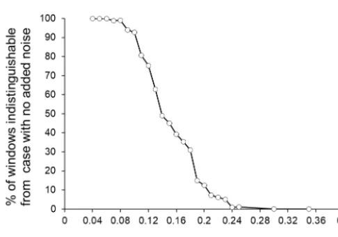
Thus, in order to ensure that the multivariate method used here enables us to discriminate between different conditions of dynamical systems, we use 3-D models in which the dy-namical features are changed from more regular to more ran-domised conditions by adding some extent of noises. We start with the Lorenz system (Fig. 3) and then proceed to the crack fusion model (Czechowski, 1991, 1993, 1995) (Fig. 4). As explained above, in both cases we add noises of different in-tensity to the original 3-D system, assuming that the more intense the added noise, the closer the model system is to randomness. Figures 3 and 4 clearly show that the number (or portion) of the 50-data windows in which the condition of the 3-D system is indistinguishable from the initial condition (the system with no added noise) gradually decreases when the intensity of the added noise is increased. This means that the method of analysis used here enables us to distinguish the conditions of systems even in cases when they are only slightly different (i.e. only a small amount of noise is added) (see the left-hand parts of the curves in Figs. 3 and 4, showing a smaller amount of added noise).
Figure 3.Percentage of the 50-data windows (shifted by 50 data steps) of the Lorenz system with added noise that are indistinguish-able from the initial condition (system with no added noise).
Figure 4.The percentage of the 50-data windows (shifted by 50 data steps) of the crack fusion model with added noise that are indis-tinguishable from the initial condition (system with no added noise).
5 Results and discussion
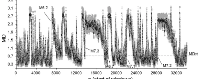
Having shown that the multivariate testing method selected for this research enables us to discriminate between different conditions of dynamical systems, we proceed to analyse data sets from the original seismic catalogue and the randomised catalogues mentioned above. We start from the case where MD values are calculated for non-overlapping, 50-data, win-dows shifted by 50 data steps, in the same way as for the 3-D model data sets. Figure 5 presents the results of this calcu-lation. Groups consisting of the ICT(i), ICD(i), and ICE(i) columns from the original catalogue were compared with the corresponding three columns of ICT(i), ICD(i), and ICE(i) data from each of 100 randomised catalogues (shuffled in time, space, and by magnitudes). In this way, the MD(i) val-ues were calculated. The MD valval-ues shown in Fig. 5 are av-erages of the MD(i)values calculated for each of the
ran-Figure 5.Seismic energy released (upper curve) and average MD values (bottom curve) calculated for consecutive non-overlapping 50-data windows shifted by 50 data steps, for the southern Califor-nia earthquake catalogue (1975–2017). Averages of the MD values and the corresponding standard deviations (given in the lower plot by white circles and grey error bars) were calculated by comparing ICT(i), ICD(i), and ICE(i) sequences in the original catalogue and in the set of randomised catalogues. The dotted line corresponds to a significant difference between windows atp=0.01.
domised catalogues. The dashed lines in this figure and the following figures indicate the critical valueFc, which was discussed in the previous section. For the number of degrees of freedom used in this research,Fc=3.99, corresponding to a significant difference between the groups withp=0.01 (MD=0.68 corresponds toFc=3.99).
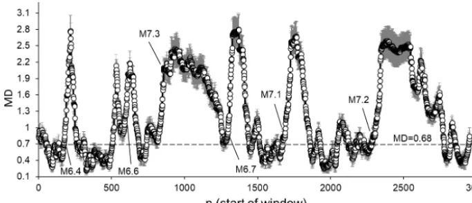
For a more precise analysis, we calculate the MD values for 50 data windows shifted by one data step (Fig. 6).
The results in Figs. 5 and 6 support the view that de-spite the generality of the background physics (Lombardi and Marzocchi, 2007; Di Toro et al., 2004; Davidsen and Goltz, 2004; Helmstetter, 2003; Helmstetter and Sornette, 2002; Corral, 2008), the processes taking place prior to and after main shocks are nevertheless different (Sornette and Knopoff, 1997; Davidsen and Goltz, 2004; Wang and Kuo, 1998). According to recent research, the latter is charac-terised by long- and short-range correlations and thus is more ordered, while the former is apparently more uncorrelated and random-like (Touati et al., 2009; Godano, 2015). Indeed, according to Bowman et al. (1998), the loss of energy (re-leased also in the form of seismic energy) that is related to the occurrence of strong events introduces memory into the system (Bowman and Sammis, 2004).
Figure 6.Average MD values calculated by comparing ICT(i), ICD(i), and ICE(i) sequences from the original SC catalogue and from the set of randomised catalogues. The dotted line corresponds to a significant difference between windows atp=0.01. MD values are calculated for 50 data windows shifted by one data step.
events. Indeed, in all windows, the seismic process, as as-sessed based on the variability in ICT(i), ICD(i), and ICE(i), after strong earthquakes is significantly different from the randomised catalogues. In contrast, the majority of the 50-data windows examined here show that the original seismic process prior to strong earthquakes is statistically indistin-guishable from the randomised catalogues (see Figs. 5 and 6). It is important to mention that the windows, located prior to strong earthquakes, make up 33 % of the total number of windows in the entire catalogue. Moreover, if we consider only those periods in the catalogue that immediately pre-cede strong earthquakes, the proportion of windows in which the seismic process is indistinguishable from randomness in-creases to 60 %–80 %. Thus, in the overwhelming majority of windows that immediately precede strong earthquakes, the seismic process is indistinguishable from that observed in the randomised catalogues. The seismic process in these parts of the original catalogue can therefore be regarded as random-like.
In order to exclude the possibility that some of the char-acteristics selected here (ICT(i), ICD(i), and ICE(i)) may have more influence on the results than the others, we carried out a similar analysis comparing groups of original and ran-domised catalogues by two of the three characteristics. The results of this separate comparison of the groups, using pairs of columns (ICT(i) and ICD(i); ICT(i) and ICE(i); ICD(i) and ICE(i)), are not shown here, but generally coincide with the results of the above analysis (using all three columns). This indicates that the results of our analysis cannot be re-duced to the influence of only a single characteristic. Thus, the changes shown in Figs. 5 and 6 reveal changes in the dy-namical features of the seismic process as whole, involving changes in all three of its domains.
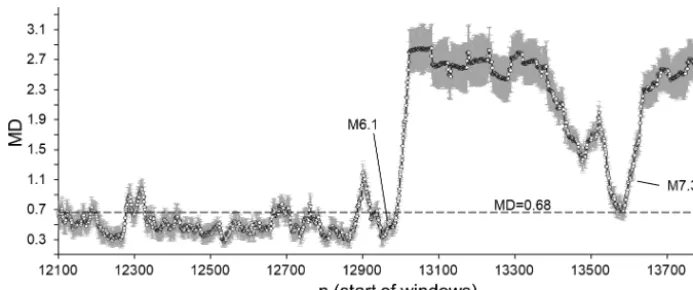
For better visualisation of the above results (see Fig. 6), Fig. 7 presents MD values calculated for 50 data windows for the period from 14 May 1990 (the window started from event 12100 in the SC catalogue) to 28 June 1992 (the
window started from event 13797 in the SC catalogue). Within this period, two strong earthquakes occurred,M6.1 (23 April 1992) andM7.3 (28 June 1992). Prior to both of these strong earthquakes, we observe windows in which the seismic process is indistinguishable from the randomised catalogues in terms of the variation in ICT(i), ICD(i), and ICE(i) data (see circles below the dotted significant differ-ence line). It is also noticeable that after these strong events, the extent of order in the seismic process strongly increases, as shown by the changes in MD values (the original catalogue becomes more different from the randomised catalogue). For M7.3, unlike the M6.1 event, this increase lasted for a considerable time after the strong event, at least until Jan-uary 1993 (see Fig. 6).
Figure 7.Average MD values calculated for the period from 14 May 1990 (12100) to 28 June 1992 (13797) in which two strong earthquakes occurred:M6.1 (23 April 1992) andM7.3 (28 June 1992). MD values are calculated by comparing ICT(i), ICD(i), and ICE(i) sequences from the original SC catalogue and from the set of randomised catalogues. The dotted line corresponds to a significant difference between windows atp=0.01. MD values are calculated for 50-data windows shifted by one data step.
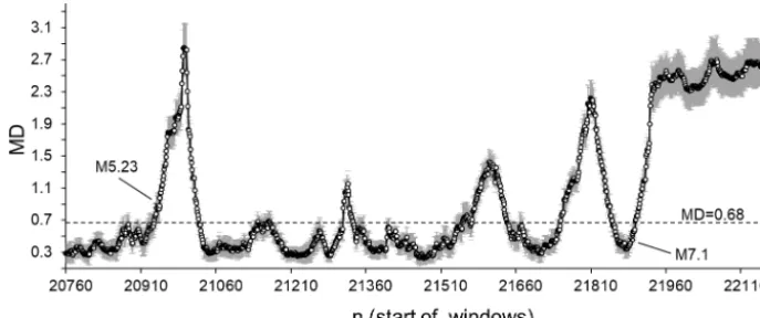
The results shown in Fig. 8 are mostly similar to those in Fig. 7. Strong and relatively strong (for this selected short period) earthquakes are preceded by a significant number of windows in which the seismic process in the original cata-logue is indistinguishable from that observed for randomised catalogues. In contrast, in all 50-data windows following strong (or relatively strong) earthquakes, we can observe a statistically significant difference. A multivariate comparison of these windows based on the variation in ICT(i), ICD(i), and ICE(i) demonstrates that in these windows, the original seismic process is significantly different from the processes taking place in the randomised catalogues (see Figs. 7 and 8).
Separate consideration of the period of the strongM7.2 earthquake occurrence leads to a similar conclusion. From Fig. 9, we can again observe that prior to strong earthquakes, the seismic process looks mostly random, and that the extent of order strongly increases after these events.
As expected, the behaviour of the seismic process prior to and following all of the strong events considered here is sim-ilar. The only difference is the length of the period during which the post-earthquake seismic process remains signifi-cantly regular compared to the randomised catalogues. For strong earthquakes, this period is clearly longer (see Fig. 6). This appears to be connected with the generation of a se-ries of aftershocks, in which the spatial, temporal, and ener-getic features are causally related to the mainshock. This is in agreement with the well-known productivity law that states that the larger the magnitude of the mainshock, the larger the total number of aftershocks (Helmstetter, 2003; Baiesi and Paczuski, 2004; Godano and Tramelli, 2016). Here, we emphasise that the question of the temporal length of the af-tershock sequence following a strong earthquake is still not understood, as it is related to the timescale of background seismic activity (Godano and Tramelli, 2016).
From Figs. 7 to 9, we can see that the extent of order in the seismic process (as assessed based on the temporal, spa-tial, and energetic distributions of earthquakes) may change not only in the periods prior to and following strong (M7.3, M7.2, and M7.1) earthquakes, but also prior to and fol-lowing other events that are not as strong, or even moder-ate. For example, as can be seen from Fig. 8, theM4.93 (14 May 1999, in window 21570) and M4.71 (24 Au-gust 1999, in window 21776) earthquakes are preceded by windows in which the seismic process mostly appears ran-dom, and are followed by windows in which the extent of order of the seismic process is markedly increased. The only difference is that for strong earthquakes, the number of win-dows in which the extent of order increases is much larger than for moderate ones. A similar conclusion can be drawn from Figs. 7 and 9. Thus, the most important conclusion is that prior to almost all strong earthquakes, in periods which can be regarded as relatively seismically calm, the original seismic process is indistinguishable from a random process, as assessed based on the MD values calculated for windows of 50-data sequences of ICT(i), ICD(i), and ICE(i) charac-teristics. In this sense, the end part of the catalogue analysed in our work (where we found a long sequence of windows (see Figs. 5 and 6) in which the seismic process is indistin-guishable from randomness, observed in a period when seis-mic activity could be regarded as relatively calm) is particu-larly interesting regarding the future activity of the fault.1
Figure 8.Average MD values calculated for the period from 24 August 1997 (20760) to 16 October 1999 (21160) in which two strong earthquakes occurred:M5.23 (6 March 1998) andM7.1 (16 October 1999). The MDs are calculated by comparing ICT(i), ICD(i), and ICE(i) sequences from the original SC catalogue and from the set of randomised catalogues. The dotted line corresponds to a significant difference between the windows atp=0.01. MD values are calculated for 50-data windows shifted by one data step.
Figure 9.Average MD values calculated for the period from 30 October 2008 (27300) to 5 April 2010 (28300) in which three moderate and strong earthquakes occurred:M5.0 (1 October 2009),M5.8 (30 December 2009), andM7.2 (4 April 2010). MDs are calculated by comparing ICT(i), ICD(i), and ICE(i) sequences from the original SC catalogue and from the set of randomised catalogues. The dotted line corresponds to a significant difference between windows atp=0.01. MD values are calculated for 50-data windows shifted by one data step.
generation is random-like, it was necessary to carry out an additional analysis of the behaviour of these small events in the case where they occur in windows after strong events. To achieve this, we selected periods of relatively low seis-mic activity, involving events with magnitudesM≤4.6. We considered 2- to 5-day periods of aftershock activity that was weaker thanM4.6 (soon after strong earthquakes). Fig-ures 10 to 12 show the results of analysis for three such periods following strong earthquakes ofM7.3,M7.1, and M7.2. As can be seen from these figures, there are no win-dows in which the original seismic process, according to MD values calculated for windows of ICT(i), ICD(i), and ICE(i) characteristics, can be regarded as random-like. In all of the windows analysed, when a clear aftershock activity follows immediately after a strong earthquake, the seismic process is significantly different from a random process. In other words, in the original catalogue, the seismic process
after strong events in periods of relatively small (M≤4.6) earthquake generation is significantly more regular than the randomised catalogues. It can also be noted that a similar sit-uation was seen for sequences of small events occurring after other strong earthquakes in the analysed catalogue. This of-fers further evidence that in periods of aftershock activity, the original seismic process is strongly different from that ob-served for the randomised catalogues in which we distorted the spatial, temporal, and energetic distribution features.
Figure 10.Magnitudes and MD values calculated for part of the SC catalogue afterM7.3 (28 June 1992, sequential number in SC cata-logue 13648) from 1 July 1992 (sequential number in SC catacata-logue 14608) to 5 July 1992 (sequential number in SC catalogue 15280). Average MD values are calculated for 50-data windows shifted by one data step; 90 % of the earthquakes in this period occurred within a distance of 0.5–70 km from the epicentre ofM7.3.
Figure 11.Magnitudes and MD values calculated for part of the SC catalogue afterM7.1 (16 October 1999, sequential number in SC catalogue 21937) from 16 October 1999 (sequential number in SC catalogue 22159) to 21 October 1999 (sequential number in SC catalogue 22697). Average MD values are calculated for 50-data windows shifted by one data step; 92 % of earthquakes in this pe-riod occurred within a distance of 1.2–60 km from the epicentre of M7.1.
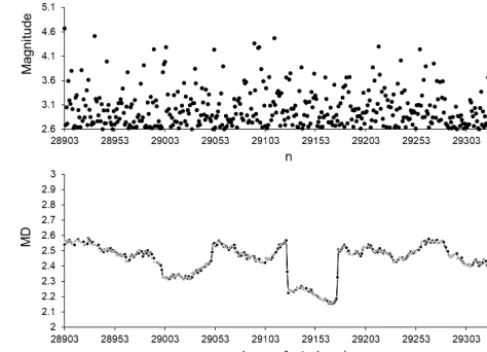
Figure 12.Magnitudes and MD values calculated for part of the SC catalogue afterM7.2 (4 April 2010, sequential number in SC cata-logue 28129) from 6 April 2010 (sequential number in SC catacata-logue 28903) to 8 April 2010 (sequential number in SC catalogue 29350). Average MD values were calculated for 50-data windows shifted by one data step; 99 % of the earthquakes in this period occurred within a distance of 0.7–60 km from the epicentre ofM7.2.
which was the closest event exceeding the selected M4.6 threshold. According to the proposed view of the time distri-bution of aftershocks, it looks very unlikely that theM5.12 earthquake could invoke aftershock activity which lasted 2 years. Thus, in agreement with our above findings, we can conclude that for the selected period, the seismic process in the original catalogue is indistinguishable from the set of cat-alogues that were randomised using a shuffling procedure in 60 % of the 50-data windows considered.
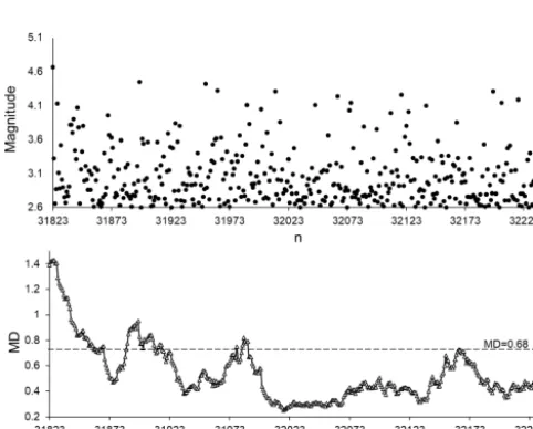
Figure 14 presents the results for the next part of the catalogue, which contained relatively small earthquakes in the observation period, which was far from the occur-rence of strong events. A moderately strong earthquake of M5.43 (7 July 2010, sequential number in SC catalogue 31011) occurred 9 months prior to the start of this 10-month long period of small earthquake activity, which lasted from 7 April 2011 (sequential number in SC catalogue 31823) to 14 February 2012 (sequential number in SC catalogue 32240). In this case, we observe that in 75 % of the 50-data windows analysed, the seismic process in the original logue is indistinguishable from the set of randomised cata-logues.
Figure 13. Magnitudes and MD values calculated for the non-aftershock part of the SC catalogue from 7 March 1983 (sequential number in SC catalogue 5000) to 5 February 1985 (sequential num-ber in SC catalogue 6253). Average MD values are calculated for 50-data windows shifted by one data step.
Figure 14. Magnitudes and MD values calculated for the non-aftershock part of the SC catalogue from 7 April 2011 (sequential number in SC catalogue 31823) to 14 February 2012 (sequential number in SC catalogue 32240). Average MD values are calculated for 50-data windows shifted by one data step.
24 May 2006 to 5 August 2007. Within this period of gen-eration of small earthquakes, 84 % of the 50-data windows indicated that the seismic activity in the original catalogue is indistinguishable from the set of randomised catalogues.
Figure 15. Magnitudes and MD values calculated for the non-aftershock part of the SC catalogue from 24 May 2006 (sequential number in SC catalogue 26259) to 5 August 2007 (sequential num-ber in SC catalogue 26717). Average MD values are calculated for 50-data windows shifted by one data step.
6 Testing the stability of the results with respect to the minimum magnitude
As can be seen from our results, as assessed based on the ICT(i), ICD(i), and ICE(i) characteristics, the seismic pro-cess of generation of relatively small earthquakes often (al-though not always) appears random and strongly depends on the space and time location of these small earthquake sequences. It can be assumed that if the observed indistin-guishability from randomness really is connected with the features of the seismic process in periods preceding strong events, then this indistinguishability should also be retained for higher values of the completeness magnitude threshold. To test this assumption, we carried out the same analysis for the SC earthquake catalogue with representative thresholds ofM3.6 and M4.6. A further increase in the threshold to M5.6 was not feasible, since only 29 earthquakes with mag-nitudes larger thanM5.6 occurred in the SC catalogue dur-ing the period considered in this research.
In Fig. 16, we give results for a completeness magnitude threshold ofM3.6. We can see that the situation for windows in which the seismicity is indistinguishable from randomness is almost exactly the same as in Fig. 6, for a completeness magnitude threshold ofM2.6. Specifically, in 33 % of all 50-data windows, the seismic process looks similar to the random process in catalogues where the dynamical structure of the original seismic process was intentionally distorted. These random-like windows in the original catalogue pre-ceded strong events.
Figure 16.Average MD values calculated by comparing ICT(i), ICD(i), and ICE(i) sequences from the original SC catalogue and from the set of randomised catalogues (completeness thresholdM3.6). The dotted line corresponds to a significant difference between windows at p=0.01. MD values are calculated for 50-data windows shifted by one data step.
Figure 17.Average MD values calculated by comparing ICT(i), ICD(i), and ICE(i) sequences from the original SC catalogue and from the set of randomised catalogues (completeness thresholdM4.6). The dotted line corresponds to a significant difference between windows at p=0.01. MD values are calculated for 50-data windows shifted by one data step. The inset shows results calculated for 30-data windows shifted by one data step.
we observe windows (of 50 data steps) in which the seis-mic process assessed based on the ICT(i), ICD(i), and ICE(i) characteristics is indistinguishable from the randomised cat-alogues. In total, 21 % of the 50-data windows had calculated MDs lower than the significance threshold value (0.68). Con-versely, at a high representative threshold (M4.6), unlike in the above cases, prior to a strongM7.1 earthquake, we do not observe 50-data windows in which the seismic process could be regarded as random.
This behaviour is apparently caused by the small number of events above the M4.6 threshold (below which, as ex-plained above, we regarded earthquakes as small, Hough and Jones, 1997) in the catalogue, and by the selected length of the window (50 data steps) for the short data sequence. In
7 Conclusions
We have investigated the variability in the regularity of the seismic process, based on its spatial, temporal, and energetic characteristics. For this purpose, we used an SC earthquake catalogue over the period 1975 to 2017. Our method of anal-ysis was a combination of multivariate Mahalanobis distance calculation and surrogate data testing. We carried out a mul-tivariate assessment of changes in the regularity of the seis-mic process, based on increments of cumulative times, incre-ments of cumulative distances, and increincre-ments of cumula-tive seismic energies calculated from the SC earthquake cat-alogue.
In order to assess the ability of the multivariate approach used here to discriminate between different conditions of namical systems, we used two 3-D models in which the dy-namical features were changed from a more regular form to more randomised conditions by adding a certain degree of noise.
It was shown that in about a third of the analysed 50-data windows, the original seismic process is indistinguish-able from a random process by the features of its tempo-ral, spatial, and energetic variability. Prior to the occurrence of strong earthquakes, in periods in which there are events with relatively small magnitudes (< M 4.6), the percentage of windows in which the seismic process is indistinguish-able from a random process increases to 60 %–80 %. At the same time, during periods of aftershock activity, the process of small earthquake generation becomes more regular in all of the windows considered and thus is strongly differentiated from the randomised catalogues.
Based on the results of our analysis, we conclude that the seismic process cannot in general be regarded either as com-pletely random or as comcom-pletely regular (deterministic). In-stead, we can say that the dynamics of the seismic process undergoes strong time-dependent changes. In other words, the regularity of the seismic process, as assessed based on the temporal, spatial, and energetic distributions, changes over time.
It was also shown that in some periods, the seismic pro-cess appears to be closer to randomness, while in other cases it becomes closer to regular behaviour. More specifically, in periods of relatively low earthquake generation activity (i.e. with smaller energy release), the seismic process looks more random, while in periods of occurrence of strong events, fol-lowed by a series of aftershocks, it shows significant devia-tion from randomness (i.e. the extent of regularity essentially increases). The period for which this deviation from random behaviour lasts depends on the amount of seismic energy re-leased by the strong earthquake. The results obtained here from a multivariable assessment of the dynamical features of the seismic process are in accordance with our previous find-ings on the dynamical changes in the temporal distribution of earthquakes (Matcharashvili et al., 2018).
It should be underlined that the occurrence in July 2019 (during the editorial process of our manuscript in NPG) of two strong earthquakes,M6.4 andM7.1, in the considered catalogue area additionally convinced us that random-like behaviour of seismic processes may indeed be regarded as one of the possible precursory markers of strong earthquakes.
Data availability. Used in this research, seismic data are available from the catalogue which is accessible from the official site (http:// www.isc.ac.uk/iscbulletin/search/catalogue/) as is mentioned in the data section. Used model data sets in case of interest can be easily modelled as they are described in Sect. 4.1 and 4.2.
Author contributions. The authors contributed in accordance with their competence in the research subject. The first author TM was responsible for all aspects of research and manuscript prepara-tion. An immense contribution by ZC helped to ensure a high mathematical and modelling level of research, and NZ contributed through programming, data analysis, and active participation in the manuscript preparation.
Competing interests. The authors declare that they have no conflict of interest.
Acknowledgements. The authors acknowledge the useful com-ments of the reviewers, Eleftheria Papadimitriou and Antonella Peresan.
Financial support. This research was supported by the Shota Rus-taveli National Science Foundation (SRNSF) (“Investigation of the dynamics of the temporal distribution of earthquakes” (grant no. 217838)).
Review statement. This paper was edited by Ilya Zaliapin and re-viewed by Eleftheria Papadimitriou and Antonella Peresan.
References
Abe, S. and Suzuki, N.: Scale-free network of earthquakes, Eu-rophys. Lett., 65, 581–586, https://doi.org/10.1209/epl/i2003-10108-1, 2004.
Baiesi, M. and Paczuski, M.: Scale-free networks of earth-quakes and aftershocks, Phys. Rev. E, 69, 066106, https://doi.org/10.1103/PhysRevE.69.066106, 2004.
Bak, P., Christensen, K., Danon, L., and Scanlon, T.: Unified scaling law for earthquakes, Phys. Rev. Lett., 88, 178501, https://doi.org/10.1103/PhysRevLett.88.178501, 2002.
pro-Christensen, K., Danon, L., Scanlon, T., and Bak, P.: Unified scaling law for earthquakes, P. Natl. Acad. Sci. USA, 99, 2509–2513, 2002.
Corral, A.: Long-term clustering, scaling, and universality in the temporal occurrence of earthquakes, Phys. Rev. Lett., 92, 108501, https://doi.org/10.1103/PhysRevLett.92.108501, 2004. Corral, A.: Scaling and universality in the dynamics of seismic
oc-currence and beyond, in: Acoustic emission and critical phenom-ena, edited by: Carpinteri and Lacidogna, Taylor and Francis Group, London, 225–244, ISBN 978-0-415-45082-9, 2008. Czechowski, Z.: A kinetic model of crack fusion, Geophys, J. Int.,
104, 419–422, 1991.
Czechowski, Z.: A kinetic model of nucleation, propagation and fu-sion of cracks, J. Phys. Earth, 41, 127–137, 1993.
Czechowski, Z.: Dynamics of fracturing and cracks, in: Theory of earthquake premonitory and fracture processes, edited by: Teis-seyre, R., PWN, Warszawa, 447–469, 1995.
Czechowski, Z.: Transformation of random distributions into power-like distributions due to non-linearities: application to geophysical phenomena, Geophys. J. Int., 144, 197–205, 2001. Czechowski, Z.: The privilege as the cause of the power
distribu-tions in geophysics, Geophys. J. Int., 154, 754–766, 2003. Davidsen, J. and Goltz, C.: Are seismic waiting time
dis-tributions universal?, Geophys. Res. Lett., 31, L21612, https://doi.org/10.1029/2004GL020892, 2004.
Di Toro, G., Goldsby, D. L., and Tullis, T. E.: Friction falls towards zero in quartz rock as slip velocity approaches seismic rates, Na-ture, 427, 436–439, 2004.
Godano, C.: A new expression for the earthquake in-terevent time distribution, Geophys. J. Int., 202, 219–223, https://doi.org/10.1093/gji/ggv135, 2015.
Godano, C. and Tramelli, A.: How long is an after-shock sequence?, Pure Appl. Geophys., 173, 2295–2304, https://doi.org/10.1007/s00024-016-1276-1, 2016.
Goltz, C. (Ed.): Fractal and chaotic properties of earthquakes, in: Lecture notes in earth sciences, Springer, Berlin, 1998.
Helmstetter, A.: Is earthquake triggering driven by small earthquakes?, Phys. Rev. Lett., 91, 058501, https://doi.org/10.1103/PhysRevLett.91.058501, 2003.
Helmstetter, A. and Sornette, D.: Diffusion of epicenters of earth-quake aftershocks, Omori’s law, and generalized continuous-time random walk models, Phys. Rev. E, 66, 061104, https://doi.org/10.1103/PhysRevE.66.061104, 2002.
Hilborn, R. C. (Ed.): Chaos and nonlinear dynamics: An introduc-tion for scientists and engineers, Oxford University Press, New York, Oxford, 1994.
Kantz, H. and Schreiber, T. (Eds.): Nonlinear time series analysis, Cambridge University Press, 1998.
Kossobokov, V. G. and Nekrasova, A. K.: Characterizing aftershock sequences of the recent strong earthquakes in Central Italy, Pure Appl. Geophys., 174, 3713–3723, 2017.
Kumar, S., Vichare, N. M., Dolev, E., and Pecht, M.: A health in-dicator method for degradation detection of electronic products, Microelectron. Reliab., 52, 439–445, 2012.
Lattin, J. M., Carroll, J. D., and Green, P. E. (Eds.): Analyzing mul-tivariate data, Thomson Brooks/Cole, Pacific Grove, CA, 2003. Lombardi, A. M. and Marzocchi, W.: Evidence of
cluster-ing and nonstationarity in the time distribution of large worldwide earthquakes, J. Geophys. Res., 112, B02303, https://doi.org/10.1029/2006JB004568, 2007.
Mahalanobis, P. C.: On tests and measures of group divergence, J. Asiat. Soci. Bengal, 26, 541–588, 1930.
Matcharashvili, T., Chelidze, T., and Javakhishvili, Z.: Nonlinear analysis of magnitude and interevent time interval sequences for earthquakes of the Caucasian region, Nonlin. Processes Geo-phys., 7, 9–20, https://doi.org/10.5194/npg-7-9-2000, 2000. Matcharashvili, T., Chelidze, T., Javakhishvili, Z., and Ghlonti, E.:
Detecting differences in dynamics of small earthquakes temporal distribution before and after large events, Comput. Geosci., 28, 693–700, 2002.
Matcharashvili, T., Zhukova, N., Chelidze, T., Founda, D., and Gerasopoulos, E.: Analysis of long-term variation of the annual number of warmer and colder days using Mahalanobis distance metrics – A case study for Athens, Physica A, 487, 22–31, 2017. Matcharashvili, T., Hatano, T., Chelidze, T., and Zhukova, N.: Sim-ple statistics for comSim-plex Earthquake time distributions, Nonlin. Processes Geophys., 25, 497–510, https://doi.org/10.5194/npg-25-497-2018, 2018.
McLachlan, G. J. (Ed.): Discriminant analysis and statistical pattern recognition, New York, Wiley, 1992.
McLachlan, G. J.: Mahalanobis distance, Resonance, 6, 20–26, 1999.
Nakamichi, H., Iguchi, M., Triastuty, H., Hendrasto, M., and Mulyana, Y.: Differences of precursory seismic energy release for the 2007 effusive dome-forming and 2014 Plinian erup-tions at Kelud volcano, Indonesia, J. Volcanol. Geoth. Res., https://doi.org/10.1016/j.jvolgeores.2017.08.004, in press, 2018. Pasten, D., Czechowski, Z., and Toledo, B.: Time series anal-ysis in earthquake complex networks, Chaos, 28, 083128, https://doi.org/10.1063/1.5023923, 2018.
Sornette, D. and Knopoff, L.: The paradox of the expected time until the next earthquake, B. Seismol. Soc. Am., 87, 789–798, 1997. Sornette, D. and Sammis, C. G.: Complex critical exponents from
renormalization group theory of earthquakes: Implications for earthquake predictions, J. Phys. I, 5, 607–619, 1995.
Taguchi, G. and Jugulum, R.: The Mahalanobis-Taguchi strategy: A pattern technology system, John Wiley and Sons, Inc., 2002.
Touati, S., Naylor, M., and Main, I. G.: Origin and nonuniversality of the earthquake interevent time distribution, Phys. Rev. Lett., 102, 168501, https://doi.org/10.1103/PhysRevLett.102.168501, 2009.