NUMERICAL MODELING OF LASER
IRRADIATION CONSIDERING
FOCAL POSITION DURING FIBER
LASER CUTTING PROCESS
DHAVAL M. PATEL
Research Scholar, Mechanical Engineering, U. V. Patel College of Engineering, Ganpat University (GNU), Kherva - 382711, Dist: Mehsana, North Gujarat. India
DR. J. L. JUNEJA
Principal, Ahmedabad Institute of Technology, Ahmedabad - 382481, Gujarat, India
DR. K. BABAPAI
Faculty of Engineering and Technology, M.S. University, Vadodara, Gujarat, India
Abstract:
Laser machining is essential in today’s advanced manufacturing, and created the need for smaller holes, smaller lands, narrower lines and spaces, smaller and more controllable spot than ever before. Study of laser beam interaction with materials enables us to explore the physical processes involved, better understands the laser machining process, and may be eliminate some unwanted side effects as well as increase efficiency of the machining process. This research attempts to reduce the experimental time and cost associated with establishing process parameters for assigning the focal spot and beam diameter. The investigation performed in this work based on the analytical and as well as experimental solutions methodology. From the readings obtained from series of experiments with 1% power should be referred for the calculation.
Keywords: Fiber Laser, Focal Position, Cutting Process
1. Introduction
The laser cutting excels in applications requiring high productivity, a high edge quality and a minimum waste, due to the fast and precise cutting process. In the last few years, the rapid development of high power fiber lasers provides more efficient, robust new technologies for materials process. A beam of coherent monochromatic light of high power density is focused on to the work piece surface causing it to vaporize locally. The material then leaves the surface in the vaporized or liquid state at high velocity [1, 2, 3]. But complete understanding of laser interaction with materials is still a matter of trials and adjustments. The real physical processes of laser beam interaction (drilling, cutting, or welding) with materials are very complex. Problem of laser interaction with materials presents many difficulties, both from modeling as well as from experimental sides. One would expect a reasonable description of the main phenomena occurring during laser interaction, but this is complicated because many of physical processes equally contribute to the development of conservation equations, producing draw back because of a great complexity of the equations to be solved. In most instances, this leads to formulation of a model needed to be solved numerically. A lack of pertinent experimental data to compare with, forces one to simplify some equations and use previous analytical and computational work done in this filed [4, 5]. Through this research work one have deduce numerical model of laser irradiation considering focal position during fiber laser cutting process.
2. Laser Interactions Modeling with Material
2.1. Mode/Diameter Consideration:-
A laser cavity is an optical oscillator. When it is oscillating there will be standing electro-magnetic wave set up within the cavity and defined by cavity geometry. Modes are the standing oscillating EM waves, which are defined by the cavity geometry. When these modes oscillate, they interfere with each other, forming the transverse standing wave pattern on any transverse intersection plane. This mechanism decides the Transverse Electromagnetic Modes (TEM) of the laser beam, which is the wave pattern on the output aperture plane. Representative TEM patterns are shown in figure 1. Clearly, the mode pattern affects distribution of the output beam energy, which affects the machining process.
Fig. 1 Representative TEM modes
But it is usually difficult to directly measure the focused beam, especially for cases when the focused spot size is below 10 microns. One solution is to combine experimental measurement with optical calculations to overcome this difficulty which incorporated in this research work.
2.2. Types of Beam:
When light passes through a limiting aperture, and it will forms a small group of rays which is called a pencil of light. Hence, it may be classified in three ways as follows:
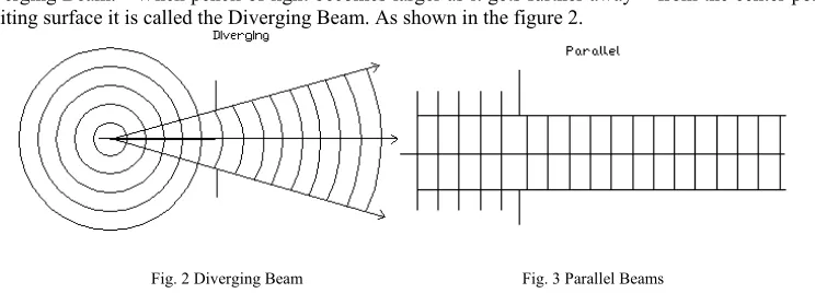
(1) Diverging Beam: - When pencil of light becomes larger as it gets further away from the center point and the limiting surface it is called the Diverging Beam. As shown in the figure 2.
Fig. 2 Diverging Beam Fig. 3 Parallel Beams
(2) Parallel Beam: - When pencil formed by the laser source becomes parallel as it gets further from the point and the limiting surface it is called the Parallel Beam. As shown in the figure 3.
Fig. 4 Converging Beam
2.3. Characteristics of Beam:
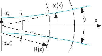
Characteristics of Beam may be as follows; as shown in the figure 5.
Fig. 5 Characteristics of Beam According to figure 5 the beam is characterize as [6]:
(1) Beam Divergence: - According to wave front propagation theory, light waves diverge, the rate at which the beam transverse is an angular term known as the divergence (θ).
(2) Beam Waist: - Point at which a beam width is at its min. size is known as the beam waist (ω0).
(3) Optics axis (Z-axis):- By measuring the beam diameter at various points along the axis of propagation known as the z-axis.
(4) Beam Quality Factor: - It is defined as the beam parameter product divided by λ/n, or it is a common measure for the beam quality of a laser beam. It is denoted as M2.
(5) Beam Radius: - At some point it will reach a minimum value, then increase with larger ‘x’, eventually becoming proportional to x. It is known as beam radius ω(x).
3. Experimental Design and Performance
3.1. Gizmo Fiber Laser Machine:
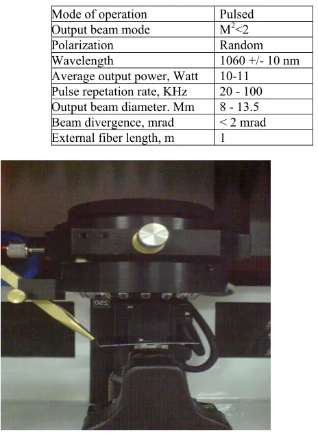
Table 1 Parameters of Gizmo Machine
Mode of operation Pulsed Output beam mode M2<2
Polarization Random
Wavelength 1060 +/- 10 nm
Average output power, Watt 10-11 Pulse repetation rate, KHz 20 - 100 Output beam diameter. Mm 8 - 13.5 Beam divergence, mrad < 2 mrad External fiber length, m 1
Fig. 6 Gizmo fiber laser machine
3.2. Experimental set up:
To find out beam diameter of laser beam all sub systems including gizmo machine are connected schematically as shown in figure 7.
Fig. 7 Schematic - Experimental Setup
4. Laser Beam Images and Measurements
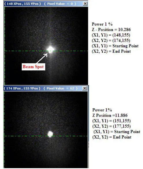
Figure 8 shows the position of beam at different Z positions and table 2 indicates readings for 1% power.
Fig. 8 Positions of beam for different Cartesian co-ordinates with respect to different Z-Position
Table 2 Data table of 1% power
Z-Position
Starting point
End point Difference
5. Analysis of Results
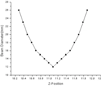
Measurements obtained through the experiment performance on the Gizmo fiber laser machine are further analyzed and converted in graphical form as shown in figure 9.
Fig. 9 Graph Z-Position vs. Beam diameter
As its clear from the graph that X-axis indicates the Z-position i.e. Optical axis of the beam, Y-axis indicates the Beam diameter of the laser beam where, the nature of graph is as polybinual (quadratic), first it is checked by best fit method (using MS-Excel). Getting beam diameter = X2-X1 then simplify it and chosen best fit curve. Hence, derived equation obtains which is best fit for the above curve.
y = 19.092x2 – 425.17x + 2379.9 (1)
Substituting the values of Z- Position in the above equation “Eq. (1)” and obtain the theoretical values of Beam diameter, mentioned in the table 3.
Table 3 Theoretical values of Beam diameter
Z-Position Beam diameter 10.286 26.5709 10.386 23.3576 10.486 20.5726 10.586 18.2162 10.686 16.2881 10.786 14.7886 10.886 13.7174 10.986 13.0748 11.086 12.8606 11.186 13.0748 11.286 13.7174 11.386 14.7886 11.486 16.2881 11.586 18.2162 11.686 20.5726 11.786 23.3576 11.886 26.5709
Now to find out exact nature of graph there are two aspects, representing (i)Polynomial Function and (ii)Equation of Parabola. Comparing both the theories, one can find that equation of parabola and simplified form of polynomial equation are similar. The equation obtained from simplification of general form of polynomial equation is,
2
2
1
2
4
x
=
by
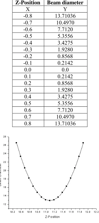
(3)From the table 3 shifting the origin (0, 0) to the point (11.086,12). Hence, table 3 can be revised as table 4. Figure 10 indicates the graph of Z-Position vs. Beam diameter from revised values derived in table 4.
Table 4 Revised values of Beam diameter
Z-Position Beam diameter X Y -0.8 13.71036 -0.7 10.4970 -0.6 7.7120 -0.5 5.3556 -0.4 3.4275 -0.3 1.9280 -0.2 0.8568 -0.1 0.2142 0.0 0.0 0.1 0.2142 0.2 0.8568 0.3 1.9280 0.4 3.4275 0.5 5.3556 0.6 7.7120 0.7 10.4970 0.8 13.71036
Fig. 10 Revised Graph of Z-Position vs. Beam diameter
Now taking the value of Z-Position as 0.1 and Beam diameter as 1 from the above table, and substituting in the equation of parabola,
2
4
x
=
by
2
2
(0.1) 4 (0.2142)
(0.1) 4(0.2142) 0.01167 b b b = = =
The focus of the obtained parabola is (0, b). Substituting the value of b in the equation of Parabola, we get
2
4
x
=
by
2
4(0.01167)
x
=
y
2
0.04668
x
=
y
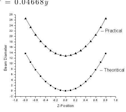
The readings obtained from the analysis of 5% Power are same as that of the reading obtained in 1% Power. The equation obtained by analyzing data of 5% Power is same as 1% Power, i.e. “Eq. (4)”.
2
0 .0 4 6 6 8
x
=
y
(4)Fig. 11 Comparison of practical and theoretical graph
From the above figure 9 & 10 it is clear that the Profile of practical graph is very much similar that of theoretical graph shown in figure 11.
6. Conclusion
Finally it has been concluded that numerical analysis of laser beam with respect to its different position, output is independent of the power reading of the machine. The purpose of numerical analysis, with laser beam and its different position, to get (establish) the equation, which is relating the optical axis and beam diameter that is,
2
0 .0 4 6 6 8
x
=
y
The above equation which is a unique result for each and every change of optical axis and that will give better result as well as better focal point with better precision.
References
[1] John C. Ion, “Laser Processing of Engineering materials”, 1st edition 2005, Elsevier Butterworth-heinemann, ISBN 0-7506-6079-1 [2] John Powell, “CO2 Laser cutting”, 1993, Springer Verlag, ISBN 3-540-19786-9
[3] Vijay Kancharla. “Fiber lasers for industrial cutting applications”, Proceedings of the 23rd International Congress on Applications of Lasers & Electro-Optics (ICALEO) 2004, Fiber & Disc Lasers pp. 18-22.
[4] Dowden, J. M., 2001, The mathematics of thermal modeling, Chapman & Hall/CRC, Boca Raton, FL.
[5] Dowden, J., P. Kapadia, and R. Ducharme, 1994, Temperature in the plume in penetration welding with a laser, Colorado Springs Conf., Colorado, Transport Phenomena in Materials Processing and Manufacturing (ASME), pp 101