Lincoln
University
Digital
Dissertation
Copyright
Statement
The
digital
copy
of
this
dissertation
is
protected
by
the
Copyright
Act
1994
(New
Zealand).
This
dissertation
may
be
consulted
by
you,
provided
you
comply
with
the
provisions
of
the
Act
and
the
following
conditions
of
use:
you
will
use
the
copy
only
for
the
purposes
of
research
or
private
study
you
will
recognise
the
author's
right
to
be
identified
as
the
author
of
the
dissertation
and
due
acknowledgement
will
be
made
to
the
author
where
appropriate
you
will
obtain
the
author's
permission
before
publishing
any
material
from
the
dissertation.
Prognostic modelling of sea level rise for the
Christchurch coastal environment
A dissertation
submitted in partial fulfilment
of the requirements for the Degree of Master of Applied Science
at
Lincoln University
by
Ashton Eaves
Abstract of a thesis submitted in partial fulfilment of the
requirements for the Degree of Master of Applied Science.
Prognostic modelling of sea level rise for the Christchurch coastal environment
by
Ashton Eaves
Prognostic modelling provides an efficient means to analyse the coastal environment and provide effective knowledge for long term urban planning. This paper outlines how the use of SWAN and Xbeach numerical models within the ESRI ArcGIS interface can simulate geomorphological evolution through hydrodynamic forcing for the Greater Christchurch coastal environment. This research followed the data integration techniques of Silva and Taborda (2012) and utilises their beach morphological modelling tool (BeachMM tool). The statutory requirements outlined in the New Zealand Coastal Policy Statement 2010 were examined to determine whether these requirements are currently being complied with when applying the recent sea level rise predictions by the Intergovernmental Panel on Climate Change (2013), and it would appear that it does not meet those requirements. This is because coastal hazard risk has not been thoroughly quantified by the installation of the Canterbury Earthquake Recovery Authority (CERA) residential red zone. However, the Christchurch City Council’s (CCC) flood management area does provide an extent to which managed coastal retreat is a real option. This research assessed the effectiveness of the prognostic models, forecasted a coastline for 100 years from now, and simulated the physical effects of extreme events such as storm surge given these future predictions. The results of this research suggest that progradation will continue to occur along the Christchurch foreshore due to the net sediment flux retaining an onshore direction and the current hydrodynamic activity not being strong enough to move sediment offshore. However, inundation during periods of storm surge poses a risk to human habitation on low lying areas around the Avon-Heathcote Estuary and the Brooklands lagoon similar to the CCC’s flood management area. There are complex interactions at the Waimakariri River mouth with very high rates of accretion and erosion within a small spatial scale due to the river discharge. There is domination of the marine environment over the river system determined by the lack of generation of a distinct river delta, and river channel has not formed within the intertidal zone clearly. The Avon-Heathcote ebb tidal delta aggrades on the innner fan and erodes on the outer fan due to wave domination. The BeachMM tool facilitates the role of spatial and temporal analysis effectively and the efficiency of that performance is determined by the computational operating system.
Acknowledgements
Table of Contents
Prognostic modelling of sea level rise for the Christchurch coastal environment ... i
Prognostic modelling of sea level rise for the Christchurch coastal environment ... ii
Table of Contents ... iv
List of Tables ... vi
List of Figures ... vii
Chapter 1 Introduction ... 1
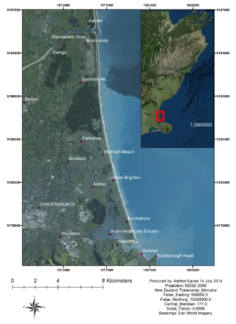
1.1 Study area ... 1
Chapter 2 The geographical setting ... 4
2.1 Geomorphology ... 4
2.2 Hydrology ... 9
2.3 Sea level rise ... 10
2.4 Earthquake effects ... 13
Chapter 3 Previous coastal modelling of the study area ... 15
3.1 The Delft3D model ... 15
3.2 The passive inundation approach and the Bruun Rule ... 16
Chapter 4 Urban planning and statutory requirements ... 20
Chapter 5 Methods and materials ... 23
5.1 Raster grids ... 25
5.2 Hydrological and climatic parameters ... 28
5.3 Simulation time interval and alternative XBeach settings ... 29
5.4 Simulations ... 30
5.5 Calibration, assumptions and related limitations of the models ... 32
Chapter 6 Results ... 34
6.1 SWAN wave propagation model ... 34
6.2 BeachMM tool ... 35
6.2.1 Sedimentation and Erosion ... 35
6.2.2 Future water level ... 40
7.1 The effectiveness of the predictive computer models for the hazard assessment of the
Christchurch coastal zone ... 44
7.2 The extent of the Christchurch shoreline in 100 years ... 45
7.3 The effects of future storm surge ... 46
7.3.1 Coastal geomorphology and fluvial processes ... 48
7.3.2 The BeachMM tool ... 49
7.3.3 Limitations ... 49
Chapter 8 Conclusion ... 51
Appendix A SWAN input file for the future maximum ... 52
Appendix B XBeach input file for the future maximum ... 53
Appendix C Effects of sea level rise for the Avon-Heathcote Estuary reported by Tonkin and Taylor (2013) ... 55
Appendix D Effects of sea level rise for the Sumner area reported by Tonkin and Taylor (2013) .... 57
Appendix E Christchurch City Council Flood management areas 2012 (Christchurch City Council, 2012) ... 58
Appendix F Calibration results from the SWAN GUI of hydrodynamic forcing for observed conditions. ... 61
List of Tables
Table 3.1 Summary of estimated shoreline retreat due to sea level rise (Tonkin and Taylor Ltd,
2013). ... 19
Table 3.2 Summary of inundation impacts for the Lower Avon and Heathcote Rivers (Tonkin and Taylor Ltd, 2013). ... 19
Table 4.1 Coastal landform sensitivity to climate change (Ministry for the Environment, 2008). ... 22
Table 5.2.1 Parameters used in the simulations. ... 28
Table 5.2.2 Water level calculations given different scenarios. ... 29
Table 5.2.3 Tide data for Lyttelton (LINZ, 2013b). ... 29
Table 5.4.1 Simulations for the future maximum scenario. ... 30
List of Figures
Figure 1.1 The numerical modelling extent of eastern Christchurch. ... 3 Figure 2.1.1 The Holocene transgression and progradation of the Christchurch shoreline (Brown &
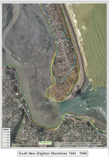
Weeber, 1992). ... 6 Figure 2.1.2 The migration of the distal end of the New Brighton Spit between 1940 and 1994.
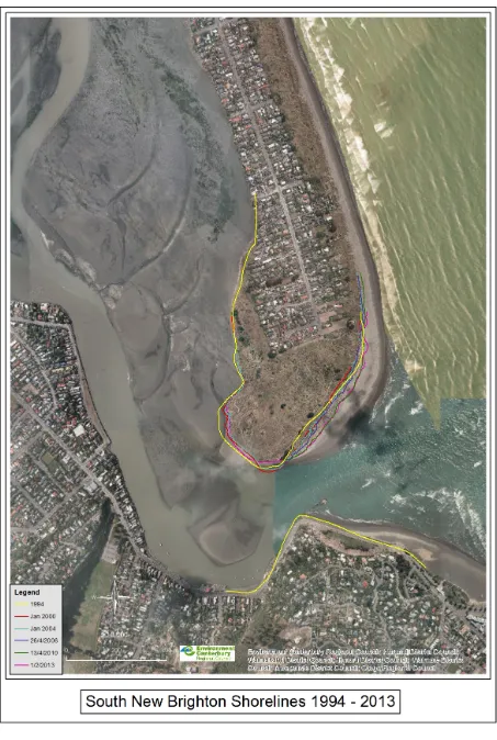
Map courtesy of Bruce Gabites at Environment Canterbury (ECan). ... 7 Figure 2.1.3 The migration of the distal end of the New Brighton Spit between 1994 and 2013.
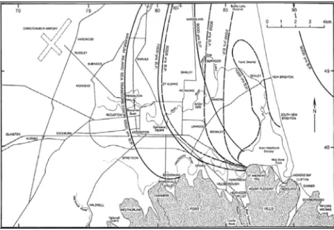
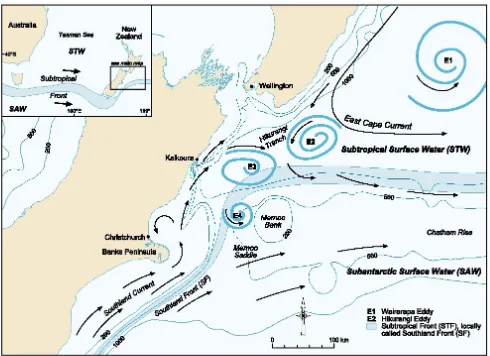
Map courtesy of Bruce Gabites at ECan. ... 8 Figure 2.2.1 East coast ocean current systems of central New Zealand. Reproduced with
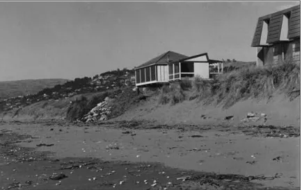
permission from Hart et al. (2008). ... 10 Figure 2.3.1 Erosion at Torea Lane in 1977. Photo taken from Southshore Residence Association
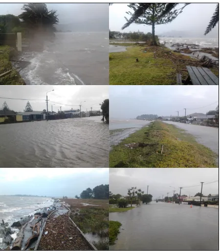
History Group (2006). ... 12 Figure 2.3.2 Personal observations of high water levels and inundation at Southshore on the 5th
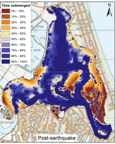
of March 2014. ... 13 Figure 3.1 Post earthquake Avon-Heathcote Estuary with percentage of bed submersion
(Measures et al. 2011). ... 16 Figure 3.2 The general response of coastal geomorphology to sea level rise, adapted by the
Ministry for the Environment (2008). The Bruun rule is outlined by the sandy coast scenarios. ... 18 Figure 5.1.1 BeachMM tool input grid: grid size = 222 by 140; cell size = 500 m by 500 m; origin = x
= 1574004.11, y = 5146388.554. ... 27 Figure 5.1.2 BeachMM tool Avon-Heathcote computational grid: grid size = 274 by 215; cell size =
25 m by 25 m; origin = x = 1575310, y = 5175832.801. ... 27 Figure 5.4.1 A flow diagram showing the pre and post processing tools used for analysis. ... 32 Figure 6.1 SWAN propagation of the significant wave height (H sig) for a) the present mean
simulation, and b) the present storm simulation. ... 34
Figure 6.2.1.1 Minimum predicted net sedimentation and erosion for East Christchurch over
100 years. Complex changes in sediment occur at the Avon-Heathcote ebb tidal delta and Scarborough Head. ... 37
Figure 6.2.1.2 Maximum predicted net sedimentation and erosion for East Christchurch over
100 years. Complex changes in sediment occur at the Avon-Heathcote ebb tidal delta and Scarborough Head. ... 38
Figure 6.2.1.3 Maximum predicted net sedimentation and erosion for the Waimakariri
coastal zone over 100 years. Complex changes in sediment occur at the river mouth with sediment plumes in the nearshore eroded and deposited on the beach face. ... 39
Figure 6.2.2.1 Inundation scenarios modelled under storm conditions for East Christchurch
given a sea level rise for 100 years of 0.23 m (min) and 0.98 m (max), a storm surge of 0.77 m, during a MHWS of 1.19 m. Inundation propagates inland beyond the study area.... ... 41
Figure 6.2.2.2 Inundation scenarios modelled under mean conditions for East Christchurch
given a sea level rise for 100 years of 0.23 m (min) 0.98 m (max). Inundation is
minimal under mean conditions. ... 42
Figure 6.2.2.3 Inundation scenario for the Waimakariri coastal environment under storm
Chapter 1
Introduction
The effective management of the coastal environment requires robust scientific analysis and detailed planning. To understand the future consequence of sea level rise on coastal environments, the use of predictive models provides the ideal platform for anticipating the impacts. Predictive models create the opportunity to simulate and understand the physical processes affecting the coastal environment and give decision makers valuable quantitative information about a range of coastal conditions (Silva and Taborda, 2012) . Geographic Information Systems (GIS) provide spatial analysis and data integration techniques for accurate mapping and analysis of coastal features (Allen, Oertel & Gares, 2012). When GIS is used in combination with statutory guidance and legislative tools of the New Zealand Coastal Policy Statement 2010 (NZCPS 2010) it enables regional and territorial authorities to provide prudent, efficient and effective outcomes for coastal management.
The Intergovernmental Panel on Climate Change (IPCC) has proposed that the rate of global sea level rise that has occurred since the mid-19th century was larger than the mean rate of the previous two millennia (IPCC, 2013). During the period from 1901-2010 the global mean sea level has risen by 0.19 m (IPCC, 2013), or an estimated mean global rate of 1.7–1.8 mm a-1 during the last century (Gehrels,
Hayward, Newnham, & Southall, 2008). Over the past 7000 years the sea level around New Zealand has remained relatively stable until recently where a rapid rise has occurred evident from saltmarsh cores from southern New Zealand (Gehrels et al. 2008).
The fundamental aim of this research project was whether the current residential zoning of Greater Christchurch meets the obligations outlined in the NZCPS 2010 for future sea level rise. Other research questions to be answered were:
• What is the effectiveness of the predictive computer models SWAN and XBeach for hazard
assessment of the Greater Christchurch coastal zone?
• What will the extent of the Greater Christchurch shoreline be in 100 years?
•
What will be the effects of storm surge given this futuristic scenario?• How will the flow discharge of the Waimakariri River effect the coastal environment?
1.1
Study area
Chapter 2
The geographical setting
Pegasus Bay has been in a progradational state since the last Holocene high stand some 8000 years ago (Schulmeister & Kirk, 1997). Relic shorelines are observable as a series of ridges and swales along the backshore of Pegasus Bay in areas where there has been minimal anthropogenic development. These patterns are treated as a record of horizontal shoreline progradation as well as of vertical sea-level rise (Allen et al. 2012). The New Brighton sand spit confines the Avon-Heathcote Ihutai Estuary, which is nourished primarily by sediments debouched by the Waimakariri River that migrate under hydrodynamic forcing. The sediment budget for the coastal environment is partially controlled by patterns of sediment transport which are governed by wave climate and sea level rise (Allen et al. 2012).
The main factors causing significant morphological change within the coastal environment are: long duration swell events, coupled with onshore winds; sediment supply, storm surges and the elapsed time between storm events (Backstrom, Jackson and Cooper, 2009), tidal range, tectonic forcing and geology. Morphological variations of the beach face, foreshore and seabed are strongly connected to the marine forcing mechanisms, particularly the wave action as the foremost factor contributing to coastal morphodynamics (Silva & Taborda, 2012). The morphologic change is not entirely related to oceanographic forcing, as extensive nearshore and shoreface accretion and erosion occurs under calm conditions, or modal high-energy conditions (Backstrom et al. 2009).
Sea level rise in southern New Zealand is higher than the global average, which can be attributed to regional thermal expansion related to the concurrent rise in global temperatures (Gehrels et al. 2008). The global mean sea level rise is anticipated to continue during the 21st century, the rate of which will very likely exceed that observed during 1971–2010 due to increased warming of the ocean and increased loss of ice mass from glaciers sheets (IPCC 2013).
2.1
Geomorphology
addition to Pegasus Bay, having formed during the past thousand years; it extends south to enclose the estuary (Hart et al. 2008). Figure 2.1.1 shows the transgression and progradation of the Christchurch shoreline. More recent migrations of the distal end of the New Brighton Spit from 1940 to 2013 are shown in figures 2.1.2 and 2.1.3. The progradation of Pegasus Bay is due to the inability of the marine environment to remove wave-eroded sediment from the floor of the bay, leading to gradual nearshore aggradation which is then transported landward to form a new berm (Schulmeister & Kirk, 1997) . However, this wave dominated environment is strong enough to disperse river derived sediment from the Waimakariri, Ashley and Waipara rivers across the nearshore of Pegasus Bay (Schulmeister & Kirk, 1997).
2.2
Hydrology
Pegasus Bay is sheltered from the predominant hydrodynamic forcing provided by the Southland Current from the south-west. This leads to nourishment of the bay via an eddy in the current; where sediment is dragged north from the Canterbury Bight and settles under calmer conditions (Brown, 1976; Hart et al. 2008; Schulmeister & Kirk; 1997). The Southland Current drives sediment south along the shore in the southern extent and north in the northern extent of Pegasus Bay (Hart et al. 2008). The Southland Current also creates an offshore banner bank at the north-eastern tip of Banks Peninsula (Hart et al. 2008). Within Pegasus Bay, long-shore sediment transport, or net sediment transport, occurs in both north and south directions due to the absence of a dominant drift direction which is dependent on the planform equilibrium of the bay (Brown, 1976). Thus, sediment transport is determined by incident wave angle and ocean current. The ocean currents for the region are outlined by figure 2.2.1.
Figure 2.2.1 East coast ocean current systems of central New Zealand. Reproduced with permission from Hart et al. (2008).
2.3
Sea level rise
and inundation at Southshore during an extreme storm in Christchurch on the 5th of March 2013, where 112 mm of precipitation was recorded over 4 days (Middlemiss, 2014).
Sea levels in New Zealand have remained relatively stable throughout the late Holocene, although a recent rapid rise has occurred given evidence from salt-marsh cores in southern New Zealand (Gehrels et al. 2008). Hannah (2004) estimated a rate of sea-level rise of 2.8 ± 0.5mm yr-1 for 20th
century New Zealand which was a considerably higher rate than that for preceding centuries. This was comparable with the nearest reliable tide-gauge at Lyttelton, 4 km south of the study site, where
a rise of 2.1 ± 0.1 mm a -1 between 1924 and 2001 was recorded (Gehrels et al. 2008; Hannah, 2004).
This rate is higher than the global average of 1.7 – 1.8 mm a-1, which can be attributed to regional
thermal expansion (Gehrels et al. 2008). Ocean warming will be greater at depth in the Southern Ocean, with best estimates of ocean warming at a depth of about 1000 m by 0.3°C to 0.6°C by the end of the 21st century (IPCC, 2013). The IPCC (2013) has estimated that the mean rate of global
averaged sea level rise was approximately 1.7 mm a-1 for the period 1901 and 2010, 2.0 mm a-1
between 1971 and 2010 and 3.2 mm a-1 between 1993 and 2010, with glacier mass loss and ocean
thermal expansion accounting for 75% of this change since the early 1970’s.
Figure 2.3.2 Personal observations of high water levels and inundation at Southshore on the 5th of March 2014.
2.4 Earthquake effects
~20-40% of its surface area, and a general tilting of the estuary that has seen subsidence to the northern extent and uplift at its southern extent of approximately 1 m and a reduction in tidal area (Measures et al. 2011).
Earthquakes affect both the morphology and evolution of coastlines by introducing abrupt elevation
changes of uplift, or subsidence, slumping or tsunami inundation (Cundy et al. 2000). The Napier
earthquake of 1931, with a magnitude of 7.8, altered the coastal morphology of the region considerably due to fault movement occurring only 30 km north-west of Napier City, which itself straddles the coast (Komar, 2010). The along-coast land elevation changes at its greatest extent saw uplift of 2 m at Tongoio, 1.8 m in Napier, and 1 m subsidence at Haumoana, Te Awanga and Clifton. Interestingly the earthquake caused abrupt uplift of the Ahuriri lagoon, reducing its area by
approximately 12.8 km2, which has since become the site of the Napier Airport (Komar, 2010).
Similarly, the Gulf of Atalanti, Greece endured significant coastal change during an earthquake series in 1894 which was dominated by a 6.2 magnitude event followed by a 6.9 magnitude event (Cundy et al. 2000). This earthquake series led to extensive coastal slumping, surface faulting, tsunami
inundation and coastal subsidence by as much as 1 m (Cundy et al.2000). Coastal subsidence was
Chapter 3
Previous coastal modelling of the study area
3.1
The Delft3D model
Figure 3.1 Post earthquake Avon-Heathcote Estuary with percentage of bed submersion (Measures et al. 2011).
3.2
The passive inundation approach and the Bruun Rule
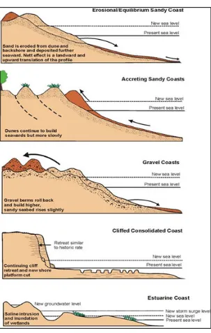
Ministry for the Environment (2008) is the Bruun Rule (1962). This model was deemed suitable by the Environment Court (Skinner v Tauranga District Council A163/02) as a precautionary approach to coastal hazard planning for an open coast beach. It is illustrated in the ‘Erosional /equilibrium sandy coast’ plate in figure 3.2. However, this simple two-dimensional model assumes: a closure depth of offshore sediment exchange, no onshore or offshore gains or losses, no long term seasonal anomaly, instantaneous response to sea level change, and no account of sediment characteristics (Tonkin and Taylor Ltd, 2013).
Figure 3.2 The general response of coastal geomorphology to sea level rise, adapted by the Ministry for the Environment (2008). The Bruun rule is outlined by the sandy coast scenarios.
utilises an inundation level of 3.3 m above Lyttelton Vertical Datum 1937 (LVD37) and the passive inundation method. This inundation level was based on a MHWS 1.15 m above LVD37 mean sea level that is exceeded 10% of the time and a sea level rise of 1.0 m, giving a passive inundation level of 2.15 m, and thus the MHWS level in 2115 would be the 2.2 m contour (Tonkin and Taylor Ltd, 2013).
Table 3.1
Summary of estimated shoreline retreat due to sea level rise (Tonkin and
Taylor Ltd, 2013).
Site ECan Profile Dune
height (m)
Slope Sea level
rise (m) Shoreline Retreat (m) Shoreline Retreat range (m)
Spencer Park C1755 5.0 0.01 1.0 70 30-100
Bottle Lake C1400 9.0 0.01 1.0 70 30-100
Effingham Street, North
New Brighton
C1065 5.1 0.01 1.0 70 30-100
Rawhiti Road, New
Brighton C0952 8.3 0.01 1.0 60 30-80
Rodney Street, New
Brighton C0815 8.6 0.01 1.0 60 30-80
Jellico Street, South New
Brighton
C0600 8.7 0.01 1.0 60 30-80
Heron Street,
Southshore C0471 6.9 0.01 1.0 60 30-90
Site Dune height
(m) Nearshore slope Sea level rise (m) Shoreline retreat (m) Shoreline retreat range (m)
Scarborough 3.9 0.016 1.0 60 30-90
Taylor’s Mistake 4.6 0.025 1.0 40 20-60
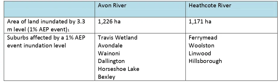
Table 3.2
Summary of inundation impacts for the Lower Avon and Heathcote Rivers
(Tonkin and Taylor Ltd, 2013).
Avon River Heathcote River
Area of land inundated by 3.3 m level (1% AEP event)1
1,226 ha 1,171 ha
Suburbs affected by a 1% AEP
event inundation level Travis Wetland Avondale
Chapter 4
Urban planning and statutory requirements
The effects of a rising sea level require the implementation of effective coastal planning and forecasting of which areas are likely to be directly affected. This hypothesised increasing trend also means the definition of realistic, rather than nominal, planning timeframes becomes abundantly more important than it has previously been (NIWA MWH GNS and BRANZ, 2012). The NZCPS 2010 has a number of directives that require action by regional and territorial authorities in order to address expected coastal changes. These objectives and policies initiated by the New Zealand Government (2010) are:
•
Objective 5: To ensure that coastal hazard risks taking account of climate change, are
managed by: locating new development away from areas prone to risks; considering
responses, including managed retreat, for existing development in this situation; and
protecting or restoring natural defences to coastal hazards
(NZCPS 2010, p. 10).
•
Policy 6: (1) (i) set back development from the coastal marine area and other water
bodies, where practicable and reasonable, to protect the natural character, open
space, public access and amenity values of the coastal environment
(NZCPS 2010, p.
13).
•
Policy 24: Identification of coastal hazards (1) Identify areas in the coastal
environment that are potentially affected by coastal hazards, giving priority to the
identification of areas at high risk of being affected. Hazard risks, over at least 100
years, are to be assessed having regard to: (a) physical drivers and processes that
cause coastal change including sea level rise; (b) short-term and long-term natural
dynamic fluctuations of erosion and accretion; (c) geomorphological character; (d)
the potential for inundation of the coastal environment, taking into account potential
sources, inundation pathways and overland extent; (e) cumulative effects of sea level
rise, storm surge and wave height under storm conditions; (f) influences that humans
have had or are having on the coast; (g) the extent and permanence of built
Planning and engineering design has historically focussed on extremes in climate variability due to the slow rate of sea level rise and therefore parameters were considered to be stationary (Ministry for the Environment, 2008). Now, planning timeframes have had to adapt to the increasing sea level using practical high tide levels such as MHWS tide being exceeded 10% of the time, and estimates of extreme high storm tides (Ministry for the Environment, 2008). However, global climate change has been increasingly well documented, regional impacts and changes can be less well quantified and differ between regions leading to subjective interpretations of the future risk (Reisinger, 2009). Key vulnerabilities from potential changes can be identified as: the magnitude of the impact on people, the environment, or cost; its timing; its persistence or reversibility; the potential for adaptation; who is most affected; the probability of occurrence; and the intrinsic importance of the impact (Reisinger, 2009). Due to the lag in system response, taking action now to create a fall in atmospheric temperature now would not see a change in sea levels for centuries to come (Reisinger, 2009). The Ministry for the Environment (2008) has classified a range of coastal landforms and their sensitivity to climate change by assessing the interrelationships between geomorphology, sediment and human influences. These are visible in table 4.1.
Table 4.1
Coastal landform sensitivity to climate change (Ministry for the
Environment, 2008).
Landform type Sea-level rise Storm surge Precipitation Wave height Wave
direction
Simple cliff High Moderate Moderate High Low
Simple landslide High Low High High Low
Composite cliff Moderate Low Moderate High Low
Complex cliff Moderate Low High High Low
Relict cliff High Low High High Low
Embryonic dunes High High Low High Low
Foredunes High High Moderate High Low
Climbing dunes Moderate Moderate Moderate Moderate Low
Relict dunes Low Low Moderate Low Low
Parabolic dunes Moderate High Low High Low
Transgressive dunes Moderate Moderate Low Moderate Low
River delta High High Moderate High Moderate
Tide dominate delta High High Low High Moderate
Wave dominated delta High High Low High Low
Shore platform High Moderate Low High Low
Sandflats High High Low High Low
Mudflats High High Low High Moderate
Pioneer saltmarsh High High Moderate High Low
Saltmarsh High High Moderate High Low
Sand beach Moderate Moderate Low Moderate High
Gravel beach Moderate Moderate Low High Moderate
Mixed beach Moderate Moderate Low High Moderate
Composite beach Moderate Moderate Low High Moderate
Boulder beach Low Low Low Moderate Low
Barrier island High High Low High High
Barrier beach High High Low High High
Spit High High Low High High
Chapter 5
Methods and materials
To achieve the research questions the numerical models of SWAN and XBeach were incorporated into the ArcGIS platform via the BeachMM tool to calculate coastal evolution and inundation. The methods used follow those created by Silva and Taborda (2012) and were adapted for the Christchurch coastal environment over a longer time period. Silva and Taborda (2012) developed the Beach Morpho-Modelling Tool Version 1.1 (BeachMM tool), a python interface to link the numerical models and the GIS environment. The models were run utilising local parameters for the present scenario to validate the model output, and again for an estimated sea level projection of 100 years from now given NZCPS 2010 directives and IPCC 2013 predictions. Two of the IPCC projections were used to promote their minimum and maximum predictions. Mean conditions and conditions under storm surge events were simulated to account for the effects of sea level rise and anomaly storm scenarios. The study area was divided into two grid extents, one focussing on the Avon-Heathcote Estuary, and the other focussed on the Waimakariri River mouth. The Waimakariri River extent was only run under the maximum IPCC (2013) projection.
McCall, 2010) . It has been successfully field tested and validated for a number of sites throughout Europe under a wide range of environmental conditions (Silva & Taborda, 2012). The BeachMM tool is a relatively new geoprocessing tool that integrates these two numerical models into the ArcGIS platform using Python script language, streamlining the process and utilising Python’s object-orientated and cross-platform capacity for modelling beach morphodynamics (Silva & Taborda, 2012). The application of this tool simplifies dataflow, permits tight coupling, minimises human error, and allows for enhanced visualisation of results (Silva & Taborda, 2012). The integration of these tools for coastal modelling provide for a seamless integration of geospatial data, automates the model chain, and enables extensive visualisation and analysis of the model results (Silva & Taborda, 2012). The schematic approach outlined in figure 5.1 illustrates how the BeachMM tool integrates into the ArcGIS platform. It shows the process by which the BeachMM tool calls SWAN and XBeach numerical models within the ArcGIS platform and the dataset flow required to operate the model.
Figure 5.1 Schematic diagram of the process employed by the BeachMM tool (Silva & Taborda, 2013).
provide a seamless transition of offshore, nearshore and terrestrial surfaces within the DEM. A coarse input grid was then used to generate the boundary conditions for the finer computational grid, utilising nesting capabilities. The BeachMM tool performed four main tasks: 1) conversion between GRID and ASCII raster formats; 2) automation of input parameters; 3) output results into an ArcGIS compatible format; and 4) calling the external models to operate in ArcGIS (Silva and Taborda, 2013). The IPCC sea level rise predictions are driven by greenhouse gas concentration trajectories, or Representative Concentration Pathways (RCPs), that are determined by estimates of future emissions. To give an overall view, the minimum and maximum RCP values were modelled. Thus,
“the global mean sea level rise for 2081−2100 relative to 1986–2005 will likely be in the ranges of 0.26 to 0.55 m for RCP2.6, and for RCP8.5, the rise by the year 2100 is 0.52 to 0.98 m, with a rate during 2081–2100 of 8 to16 mm a -1. These ranges are derived from CMIP5 climate projections in
combination with process-based models and literature assessment of glacier and ice sheet contributions” (IPCC, 2013). Therefore a lower value of 0.26 m and an upper value of 0.98 m were used. SWAN and XBeach were executed with mean and significant storm data from the Canterbury offshore wave buoy.
5.1
Raster grids
The development of a seamless topobathy follows a similar technique used by Allen et al. (2012) where the integration of topographic and bathymetric data derived a triangular irregular network (TIN) and in turn a rasterized DEM. Generation of bathymetric bottom grids on which to run SWAN and XBeach were developed by merging the following files:
• Terrestrial LiDAR data was obtained from Lincoln University. This airborne laser scanning survey was conducted over Christchurch City and Lyttelton from 20th - 30th May 2011, and was designed to support the February 2011 earthquake recovery effort (AAM Pty Ltd, 2011). It captured a vector terrain model with an average point separation of 0.5m with ground support provided by GeoSystems NZ by way of GNSS base stations to assess the accuracy (AAM Pty Ltd, 2011).
• Bathymetric vector contours and hydro sounding points were obtained from the Land
Information New Zealand (LINZ) data service (LINZ, 2013a).
• New Zealand geographic contours were also obtained from the LINZ data service (LINZ,
2013a) for terrestrial values outside the LiDAR dataset required by the grid.
then reformatted into ESRI GRID. Distortion created over terrestrial values created by the TIN outside the area of the LiDAR area were ignored but necessary as this space needed to be occupied in order for the XBeach model to run. The same process was used to create the larger input grid extent used by SWAN for hydrodynamic forcing. This extent was 110 km by 70 km and encompasses part of Banks Peninsula and the Pegasus Canyon. The study area comprised two computational grids, one centred on East Christchurch and encompassing the Avon-Heathcote Estuary, where the other focussed on the Waimakariri coastal environment.
Figure 5.1.1 BeachMM tool input grid: grid size = 222 by 140; cell size = 500 m by 500 m; origin = x = 1574004.11, y = 5146388.554.
Figure 5.1.2 BeachMM tool Avon-Heathcote computational grid: grid size = 274 by 215; cell size = 25 m by 25 m; origin = x = 1575310, y = 5175832.801.
5.2
Hydrological and climatic parameters
The SWAN hydrological input parameters were calculated from the LINZ sea level dataset (LINZ, 2013b), the Canterbury wave buoy dataset provided by ECan, and the climatic conditions were taken from NIWA’s (2013) Cliflo server. The wave buoy dataset starts in February 1999 and ends in July 2013 with measurements taken approximately every half hour. It is moored 17 km east of Le Bons Bay, Banks Peninsula with a Latitude of 43° 45' South and a Longitude of 173° 20' East in approximately 76 m of depth ensuring no interference by the seabed or terrestrial landmass with the measurements (Environment Canterbury, 2014). The Cliflo dataset was taken from the weather station at New Brighton Pier as 3-hourly measurements from the 27th of August 2009 to the 1st of January 2013.
There were two types of parameter settings used in the simulations with differing water levels over different time periods; one utilised mean hydrological and atmospheric conditions, and the other utilised the hydrological and atmospheric conditions during a storm. The parameters are: significant wave height (H sig); wave period (T); the direction from which waves propagate (Sea θ); the velocity of the wind (Wind v); and wind direction (Wind θ). For the mean forcing, the mean statistics from the various datasets were used for the parameters, except for wind direction where the mode was used. For storm forcing conditions the peak values were obtained for the different parameters during a recent storm on the 28th of June 2012, which ran over two days, and applied to the simulation. This storm is considered an extreme event as H sig falls within the top 1 % of all significant wave heights (Komar et al., 2013) and was chosen based on the availability of data for all parameters. Table 5.2.1 outlines the various parameter settings used in the simulations. Water levels have been calculated according to table 5.2.2 from data acquired from LINZ (2013b) on the Lyttelton tidal regime, IPCC predictions, and storm surge calculations, with MHWS referring to the mean high water spring tide. Table 5.2.3 outlines the tidal regime data from LINZ (2013b). Storm surge was calculated by subtracting the predicted tide level provided by LINZ (2013a) from the observed tide level recorded by the offshore wave buoy at the time of the storm. Storm surge was calculated at 0.77 m and is shown in table 5.2.2. Appendix A illustrates a SWAN input file used. The Waimakariri coastal environment simulation was operated utilising only the upper limit of the IPCC (2013) predictions of 0.98 m.
Table 5.2.1 Parameters used in the simulations.
Simulation Water
level (m) H sig (m) T (s) Sea θ (°, mode) Wind v (m s-1) Wind θ (°, mode)
Mean 0 1.95 8.8 194.2 5.11 75
Table 5.2.2 Water level calculations given different scenarios.
Present mean
(m) Present storm (m) 100 year SLR min (0.27 m) 100 year SLR max (0.98 m)
MHWS 0 1.19 1.19 1.19
Storm surge 0 0.77 0.77 0.77
SLR 0 0 0.27 0.98
TOTAL 0 1.96 2.23 2.94
Table 5.2.3 Tide data for Lyttelton (LINZ, 2013b).
Standard
Port MHWS (m) MHWN MLWN MLWS Spring Range Neap Range MSL HAT LAT
Lyttelton 2.57 2.06 0.68 0.22 2.35 1.38 1.38 2.69 0.1
River discharge was incorporated into the XBeach model by way of location and time series text files that are then called into the computational domain. These files included the location, width, and flow rate of water for the Avon, Heathcote and Waimakariri rivers. The rate for the Avon River was set at 2 m3 s-1 and for the Heathcote River at 1 m3 s-1 taken from Measures (2011). An average flow rate of
138.9 m3 s-1 was used for the Waimakariri River which was recorded at State Highway 1 and obtained
from ECan (2014).
5.3
Simulation time interval and alternative XBeach settings
Due to the long time scale of 100 years undertaken by this research, the morphological factor (morfac) available in XBeach was utilised. A morfac of 6 corresponded to 10 minutes of hydrodynamic forcing becoming 1 hour of forcing (Roelvink et al., 2010). This acceleration technique, or multiplier, sped up computation considerably, although was unreliable above 400 or near its maximum of 1000 for these simulations. The mean simulations were run at a morfac of 200, and storm simulations at a morfac of 6. Short simulations were also an issue under mean conditions as the XBeach model required a long period of time to propagate a result.
To recreate a real-world scenario, SWAN and XBeach were then run for a 10 year period, followed by a 2 day storm and repeated with increasing water levels until 100 years had passed. The division of the time period was also necessary as the XBeach program would implode with such large timeframes given the computing capacity. Therefore the 10 year simulation with a morfac of 200 was run for 1,576,800 s and the 2 day simulation with a morfac of 6 was run for 28,800 s.
computation option was set to ‘wave averaged’ (Turb=1). Longwave stirring was turned on (LWS=1). Shortwave stirring was stirred on (SWS=1). Appendix B illustrates the XBeach parameter file.
5.4
Simulations
Two grouped simulations were conducted to predict the future outcome for the Christchurch coastal environment consisting of twenty cumulative simulations with increasing water levels and intermittent storms, these were:
1. Future maximum scenario; computed with the IPCC 100 year sea level rise maximum
prediction of 0.98 m, as illustrated in table 5.4.1.
Table 5.4.1 Simulations for the future maximum scenario.
Run Forcing type Water level (m)
H sig
(m) (s) T (°, mode) Sea θ Wind v (m s-1) (°, mode) Wind θ interval Time Morfac
1 Mean 0 1.95 8.8 194.2 5.11 75 10 years 200
2 Storm 1.96 7.49 13.3 140 9.2 230 2 days 6
3 Mean 0.11 1.95 8.8 194.2 5.11 75 10 years 200
4 Storm 2.07 7.49 13.3 140 9.2 230 2 days 6
5 Mean 0.23 1.95 8.8 194.2 5.11 75 10 years 200
6 Storm 2.19 7.49 13.3 140 9.2 230 2 days 6
7 Mean 0.34 1.95 8.8 194.2 5.11 75 10 years 200
8 Storm 2.30 7.49 13.3 140 9.2 230 2 days 6
9 Mean 0.46 1.95 8.8 194.2 5.11 75 10 years 200
10 Storm 2.42 7.49 13.3 140 9.2 230 2 days 6
11 Mean 0.56 1.95 8.8 194.2 5.11 75 10 years 200
12 Storm 2.52 7.49 13.3 140 9.2 230 2 days 6
13 Mean 0.67 1.95 8.8 194.2 5.11 75 10 years 200
14 Storm 2.63 7.49 13.3 140 9.2 230 2 days 6
15 Mean 0.79 1.95 8.8 194.2 5.11 75 10 years 200
16 Storm 2.75 7.49 13.3 140 9.2 230 2 days 6
17 Mean 0.90 1.95 8.8 194.2 5.11 75 10 years 200
18 Storm 2.86 7.49 13.3 140 9.2 230 2 days 6
19 Mean 0.98 1.95 8.8 194.2 5.11 75 10 years 200
20 Storm 2.94 7.49 13.3 140 9.2 230 2 days 6
2 Future minimum scenario; computed with The IPCC 100 year sea level rise minimum
prediction of 0.27 m, as illustrated in table 5.4.2.
Table 5.4.2 Simulations for the future minimum scenario.
(m)
1 Mean 0 1.95 8.8 194.2 5.11 75 10 years 200
2 Storm 1.96 7.49 13.3 140 9.2 230 2 days 6
3 Mean 0.03 1.95 8.8 194.2 5.11 75 10 years 200
4 Storm 1.99 7.49 13.3 140 9.2 230 2 days 6
5 Mean 0.06 1.95 8.8 194.2 5.11 75 10 years 200
6 Storm 2.02 7.49 13.3 140 9.2 230 2 days 6
7 Mean 0.09 1.95 8.8 194.2 5.11 75 10 years 200
8 Storm 2.05 7.49 13.3 140 9.2 230 2 days 6
9 Mean 0.12 1.95 8.8 194.2 5.11 75 10 years 200
10 Storm 2.08 7.49 13.3 140 9.2 230 2 days 6
11 Mean 0.15 1.95 8.8 194.2 5.11 75 10 years 200
12 Storm 2.11 7.49 13.3 140 9.2 230 2 days 6
13 Mean 0.18 1.95 8.8 194.2 5.11 75 10 years 200
14 Storm 2.14 7.49 13.3 140 9.2 230 2 days 6
15 Mean 0.21 1.95 8.8 194.2 5.11 75 10 years 200
16 Storm 2.17 7.49 13.3 140 9.2 230 2 days 6
17 Mean 0.24 1.95 8.8 194.2 5.11 75 10 years 200
18 Storm 2.20 7.49 13.3 140 9.2 230 2 days 6
19 Mean 0.27 1.95 8.8 194.2 5.11 75 10 years 200
20 Storm 2.23 7.49 13.3 140 9.2 230 2 days 6
The variables that were measured by the BeachMM tool for this study were net sedimentation or erosion (sedero), bed level and water level. Each new bed level created was incorporated into the next simulation, thereby incrementally adjusting the bathymetry. The sedero output required post-processing analysis to create a fuzzy overlay in ArcGIS which summed all of the outputs created to produce the net sedimentation or erosion. The results of the final simulation were used as output for the bed level and water level due to the incremental increase. Resulting grids were then rotated back to the original space. The ArcGIS conversion tools used to generate the grid and the post processing analysis are visible in figure 5.4.1.
Figure 5.4.1 A flow diagram showing the pre and post processing tools used for analysis.
5.5
Calibration, assumptions and related limitations of the models
The model was calibrated through remote desktop application and observation as time constraints did not allow for direct field measurements. The SWAN graphic user interface (GUI) was utilised to test the hydrodynamic forcing, bathymetric grid and changing water level. This GUI allows for simplified visualisations of the resultant hydrodynamic forcing. Wave height, wave period, wind direction and wind velocity used to run the simulations were then compared with those forecasted by Meteo365 (2013) and observed from the foreshore and the surf zone. Appendix F shows calibration of the hydrodynamic forcing for recent observed conditions using the SWAN GUI.
The limitations of the SWAN and XBeach models that are relevant to their use in these simulations are to follow.
Limitations of the SWAN model:
• SWAN does not compute wave-induced currents (Booij, 2012).
• Unexpected interpolation patterns on the computational grid may arise from the differing
resolution of the input grid (Booij, 2012).
• SWAN can have convergence problems due to the iteration process (Booij, 2012).
• Unintentional coding bugs may be present (Booij, 2012).
Limitations of the XBeach model:
• XBeach does not perform well in very shallow water (Roelvink et al., 2010).
• The alongshore gradient of wave energy is zero in the stationary case (Roelvink et al., 2010).
• The computational x-axis must be orientated toward the coast and rectilinear (Roelvink et
al., 2010).
• Under sheet flow conditions, greater velocities lead to greater sediment transport rates, but not to greater equilibrium sediment concentrations (Roelvink et al., 2010).
Chapter 6
Results
6.1
SWAN wave propagation model
The results for the significant wave height of the SWAN run are shown in figure 6.1 for a) mean conditions, and b) storm conditions. The mean wave height under normal conditions approaching the shore of Pegasus Bay is 0.2 – 0.4 m, and 1 – 3 m under storm conditions. The mean period of waves
approaching the shore of Pegasus Bay is 8 – 8.5 m s-1 under normal conditions, and 11 – 12 m s-1
under storm conditions. The direction under normal conditions is 194°, and under storm conditions is 140°.
Figure 6.1 SWAN propagation of the significant wave height (H sig) for a) the present mean simulation, and b) the present storm simulation.
A.
6.2
BeachMM tool
6.2.1
Sedimentation and Erosion
The net result of all simulations for sedimentation and erosion (sedero) over the 100 year period for both the minimum and maximum scenarios illustrates a slight progradation of the foreshore with the majority of the sediment being received from the nearshore, although the minimum scenario is a magnitude smaller. The most dynamic areas are the Avon-Heathcote Estuary ebb tidal delta, the Waimakariri River mouth and the Scarborough Heads; with rates of deposition being relatively high on the western aspects and higher erosional rates on the eastern aspects of these features.
The sedimentation rate for the minimum scenario for the majority of the foreshore is 0.00002 m3 a-1
to 0.00023 m3 a-1, with pockets of erosion present throughout of 0.00031 m3 a-1 to 0.00153 m3 a-1
Sedimentation rates are higher on the western aspect of the Avon-Heathcote Estuary ebb tidal delta and at Scarborough Head ranging from 0.00023 m3 a-1 to 0.00102 m3 a-1. On the eastern aspects,
erosion rates are higher ranging from 0.00018 m3 a-1 to 0.00437 m3 a-1. The nearshore appears to
erode at a minimal rate of 0.00001 m3 a-1 to 0.00007 m3 a-1 at approximately 1 km out. These results
can be seen in figure 6.2.1.1. The mean statistic for the sedero results is negligible at -0.0001 m3, with
a standard deviation of 0.004 for the period.
The sedimentation rate under the Avon-Heathcote Estuary simulations for the maximum scenario for the majority of the foreshore is 0.00017 m3 a-1 to 0.0009 m3 a-1, with pockets of erosion present
throughout of 0.00018 m3 a-1 to 0.00041 m3 a-1. Sedimentation rates are higher on the eastern aspect
of the Avon-Heathcote Estuary ebb tidal delta and at Scarborough Head, ranging from 0.00017 m3 a-1
to 0.00162 m3 a-1. On the eastern aspects, erosion rates are higher, ranging from 0.00055 m3 a-1 to
0.00614 m3 a-1. The nearshore appears to erode at a minimal rate of 0.00007 m3 a-1 to 0.00031 m3 a-1
at approximately 1 km out. These results can be seen in figure 6.2.1.2. The mean statistic for the sedero results is negligible at -0.0001 m3, with a standard deviation of 0.006 for the period.
The sedimentation rate for the Waimakariri coastal environment also illustrates that the coast will prograde at the expense of the nearshore. The nearshore illustrates a net sediment flux of -0.00032 m3 a-1 to -0.00222 m3 a-1, whereas the beach face has undergone a deposition of 0.00031 m3 a-1 to
0.00285 m3 a-1, which is illustrated in figure 6.2.1.3. The mean statistic for the sedero results is
negligible at -0.0004 m3, with a standard deviation of 0.024 for the period.
6.2.2
Future water level
The future minimum and maximum water levels under storm conditions will lead to inundation of coastal areas of Greater Christchurch. The areas affected will primarily be around the fringes of the Avon-Heathcote Estuary, Brooklands and Kairiki due to their low topography. Sumner, the lower reaches of the Avon and Heathcote rivers, and farmland adjacent to the Brooklands lagoon will also be inundated to varying extents.
Figure 6.2.2.3 Inundation scenario for the Waimakariri coastal environment under storm
Chapter 7
Discussion
The fundamental aim of this research project was whether the current CERA zoning for Greater Christchurch meets the obligations outlined in the NZCPS 2010 for future sea level rise, and it would appear that it does not meet those requirements. This is because coastal hazard risk has not been comprehensively quantified by the installation of the CERA residential red zone. However, the CCC’s flood management area does provide an extent to which managed retreat is a real option. Development can still be undertaken on areas that are at risk from moderate predicted levels of inundation. The present MHWS level will frequently be exceeded in the future , particularly in areas with a low tidal range like those occurring through the central parts of the east coast, leading to storm inundation having greater influence and enhanced coastal erosion (Ministry for the Environment, 2008). The expected changes to atmospheric conditions, storms and cyclones will also lead to coastal erosion and inundation through changes to the wave climate and beach sediment movement (Ministry for the Environment, 2008). Local government is required to effectively identify, account, avoid and mitigate any coastal hazards, vulnerabilities, or consequences over at least a 100 year period to preserve coastal environments from inappropriate development while enhancing public access (New Zealand Government, 1991). Simulating coastal change at timescales relevant to planning and development requires new types of modelling approaches over large temporal and spatial scales, these should incorporate high quality datasets to enable the refinement, calibration and validation of such models (Ministry for the Environment, 2008).
7.1
The effectiveness of the predictive computer models for the hazard
assessment of the Christchurch coastal zone
The XBeach model performed well under open coast conditions although not so well under estuarine conditions. This is because the water level is expectedly shallow in this intertidal zone and propagation of hydrodynamic forcing is near impossible. The time interval was also an issue as the morphological updating required a certain timeframe to evolve and inhibited some application of the morphological acceleration. XBeach did perform the tasks of dune and nearshore erosion, berm and foreshore sedimentation, sea bed updating, over washes and breaches well to simulate a natural coastal response to a range of timeframes and conditions.
With any abstraction of the environment into a computerized simulation, limitations exist as common constraints arise from the scale of observation, computational limitations, uncertainty, and error propagation in GIS and its applications (Allen et al. 2012). These limitations were: the effects of interdecadal climatic oscillations such as ENSO on regional sea levels; the accuracy of models to incorporate detailed sediment flux analysis from rivers or at the grid boundary; and the amount of computing capacity. The beach MM tool needs to be programmed with a greater range of atmospheric and sea state conditions by calling a file with a diverse range of conditions over at least a decadal time period. This would help to overcome anomalies such as ENSO and southern oscillation projections that need to be included in any future study. Inclusion of the Waimakariri River sediment discharge was not applicable as this sediment has not been readily quantified and XBeach does not have the ability to input sediment at the boundary without development of the program. This research was also limited by computing capacity. Grid resolution, size and morphological updating over time were completely dependent on the computers’ virtual memory, which led to reduced grids at a lower resolution than first tested.
Overall the integration of the SWAN and XBeach model into a GIS platform through the BeachMM tool in ArcGIS proved to be very useful and powerful. SWAN provided a very stable environment on which to gather the hydrodynamic forcing dataset as it has been in creation for many years and therefore is well refined. Conversely, XBeach is a recently developed program with very little support for those choosing to operate it over a GIS platform as it has been designed to operate primarily through Matlab. As stated by Silva and Taborda (2012) the BeachMM tool does provide: seamless integration of geospatial data into existing numerical models, model chain automation, powerful visualising and analysis tools for the exploitation of model results. Furthermore, any prognostic modelling should be correlated with successive observations and monitoring to discover the model’s accuracy.
7.2
The extent of the Christchurch shoreline in 100 years
coastline will continue to prograde given sediment supply from the Waimakariri River continues. The results of this research provide a minimal amount of progradation that is likely to occur over the period as a closed system to sediment supply was modelled. Changes in the west-east gradient in rainfall will see it wetter in the west and drier in the east with an increase in rainfall intensity during severe storms (Ministry for the Environment, 2008). The catchment of the Waimakariri River extends to the main divide and receives westerly rainfall which should facilitate enhanced flow and sediment supply to the coast. As Pegasus Bay is marine dominated, where sediment can be dispersed but not removed from the nearshore ,what is not lost to deep water during storms will incrementally nourish terrestrial dunes during modal conditions (Schulmeister & Kirk, 1997) . This was indicated by the model in the absence of the Waimakariri River sediment flux as slight progradation occurred at the expense of the nearshore. Assuming replacement of this sediment by the Waimakariri sediment flux, progradation will continue to occur.
The accumulation of sediment on the inner fan of the ebb tidal delta of the Avon-Heathcote Estuary may significantly reduce channel width and depth. The reduced tidal flow may lead to the New Brighton spit making landfall on the peninsula with intermittent openings to the sea in times of flood. This has occurred on Lake Ellesmere to the south of Banks Peninsula. The New Brighton Spit has made landfall on the peninsula before to form a barrier lagoon system (Hart et al., 2008; Schulmeister & Kirk, 1997). For planning purposes spits are not landforms but mobile coastal features that are characterised by large shoreline migrations over relatively short time periods (Hart et al., 2008). Although, sea level rise could scour and deepen estuarine channels if these changes exceed sediment build up, or where sedimentation fills estuaries from enhanced rainfall events, then the estuary may cease to exist (Ministry for the Environment, 2008). Therefore close monitoring of the sedimentation of the Avon-Heathcote Estuary will help determine spatial patterns of inundation.
Estimates of Greater Christchurch coastal dune recession with sea level rise relies on an overly simplified coastal environment. The two-dimensional Bruun Rule is obsolete in predicting the
contemporary geomorphology of foredunes in response to sea level rise (Hilton, 2013). This is
because the Bruun Rule assumes unconsolidated sediment, no sediment inputs, and no net alongshore flux (Hilton, 2013). The introduced Marram grass species has forced accretion on many South Island beaches due to its efficiency at sand entrapment, this has the potential of further foredune accretion with increasing mean wind speeds (Hilton, 2013).
7.3
The effects of future storm surge
although storm surge with a MHWS tide will not be prevented from inundation of the low lying areas adjacent to the Avon-Heathcote Estuary and the Brooklands Lagoon. The lower reaches of the Avon and Heathcote Rivers are also tidal making parts of these catchments vulnerable to sea level rise, although the Christchurch earthquake of 22 February 2011 lifted the tidal portion of the Heathcote catchment by about 0.4 m and lowered the rest by 0.1-0.3 m (Tonkin and Taylor Ltd, 2013). This report describes the minimum inundation hazard zone as the 100 year maximum of 2.94 m above mean sea level outlined in figures 6.2.2.1 and 6.2.2.3, or the setback limit for development. The flood management areas assigned by the Christchurch City Council that are visible in appendix E, provide an acceptable extent by which to inhibit development and are similar to the modelled extent for the future maximum inundation during storm conditions. However, given the risk associated with future inundation, parts of these flood management areas should also be zoned red.
The maximum inundation scenario is not as great as that modelled by Tonkin and Taylor Ltd (2013) (appendices C and D) as the modelling extent was smaller and coastal processes were taken into account which limited dune overtopping and coastal erosion. Tonkin and Taylor Ltd (2013) employed the passive inundation approach which will tend to overestimate inundation (Ministry for the Environment, 2008). However, their report was more accurate in dealing with sections of the coastal environment that were backed by revetments as the coarse 25 m resolution employed by this study could not differentiate hard and soft structures without a higher resolution grid and further model programming. Tonkin and Taylor (2013) did employ a similar sea level rise that was 1.0 m by 2115. They also allowed a free board of 0.4 m to allow for localised wave effects and other uncertainties (Tonkin and Taylor Ltd, 2013).
The effects of storm surge given the futuristic Waimakariri coast scenario will see extensive flooding of Brooklands, Kairiki and the surrounding low lying area which is predominantly agricultural. Coastal lagoon topography is generally low, otherwise they would cease to exist and rivers would drain freely into the ocean. The amount of flooding modelled is a modest estimation as during a period of storm surge, precipitation is likely which would elevate the river discharge and increase the water level in the lagoon at high tide. This parameter was not included into the modelling exercise, but is worth investigating. The red zone installed by CERA (2014) at Brooklands was appropriate as this area is highly susceptible to flooding, although it needs to be extended landward. Much of the rest of this area is under agricultural landuse and therefore is at less risk than developed residential land. An expansion of the Kairiki red zone is advised.
the classification of episodic hazard events becomes very difficult with climate change, which may be exponential, parabolic or quasi-linear. The integration of GIS, satellite imagery, sensor technology and numerical modelling provides for a more objective scientific expression.
7.3.1
Coastal geomorphology and fluvial processes
The results of the BeachMM tool show that the marine environment dominates over the fluvial processes. A prominent delta failed to form in the intertidal or subtidal zone where the flow exits the Waimakariri River and the Avon-Heathcote delta is formed by the ebb tide. However, poorly-formed sediment was deposited, with incised alluvial or tidal scouring in these zones. The modelling shows that any sediment accumulating in the nearshore as a result of fluvial processes will be forced landward to the foreshore, which is then transported by aeolian mechanisms into the dune system.
The original Waimakariri DEM showed two fan deposits south of the river mouth that were eroded by hydrodynamic forcing and deposited to the foreshore by the model. It is speculated that these deposits may be the result of Waimakariri flooding events of the recent past. During peak flood events the Waimakariri River can debouch 800 m3 s-1 (Canterbury Regional Council, 2014). This could
explain the presence of these disjointed sediment deposits in the subtidal zone. Breach events of coastal barriers at river mouths inject coarse slugs of sediment into the coastal environment which nourish down-drift beaches (Hart & Bryan, 2008). Further analysis and quantification of sediment load and bed load debouching into Pegasus Bay from the Waimakariri River is required. The mouth of the Waimakariri River does not meander up and down the coast, unlike the Rakia, Rangitata, Ashburton and Waitaki (Hart & Bryan, 2008), and the Hurunui and the Ashley rivers. Reasons for this could include: anthropogenic constraints of the channel; gravel extraction in the catchment near the coast; or the long shore drift at the Waimakariri River mouth being in a state of dynamic equilibrium. Given the storm surge scenario modelled in this report, the dune system adjacent to the Brooklands Lagoon could easily be compromised during this event creating a new location for the river mouth. The Waimakariri coastal environment in 100 years will see a continuation of a slow progradation under sea level rise and assuming river flows do not decrease due water abstraction in the catchment. The domination of the marine environment will force sediment north and south of the river mouth (Schulmeister & Kirk, 1997). There is the possibility that a subtidal delta may form temporarily, to then be removed by hydrodynamic forcing over time.
marine and climatic conditions. This favours the ebb-tidal delta formation and sands spit deposition. Again, water abstraction in the catchment of the Avon and Heathcote rivers will also determine the outcome for the estuary and ebb-tidal delta.
7.3.2
The BeachMM tool
The BeachMM tool provides insight through prognostic modelling into coastal morphodynamics at varying timescales. It allows for the desktop use of a model which is usually only appropriate for super computers with abundant RAM and processing power. There are also endless options for further development through its python script language for time series animations of storms, enhanced climate and river data integration, and assessing the outcomes of Tsunamis.
The ability for the BeachMM tool to operate over both temporal and spatial scales allows users a type of GIS analysis frequently constrained to low resolution numerical models. Combining numerical models into the GIS platform allows for easily accessible high resolution spatial data to be analysed over time with different parameters. Combining the universally accepted and tested hydrodynamic SWAN model and the empirically tested geomorphological XBeach model provides the user with confidence in the results. As the BeachMM tool can run on desktop or laptop computers, this provides access of its application to a vast numbers of users. Thus providing greater accessibility than if it was to be operated via powerful super computers which are usually required for prognostic modelling.
There are endless possibilities to the advancement of the BeachMM tool due to its versatile python script. The ability to output results at incrementally varying time intervals throughout the simulation makes it possible to produce animations of hydrodynamic forcing or coastal evolution. This could also be extended to the effects of Tsunamis on the shore, although the hydrodynamics are slightly different for tsunamis and therefore may require modification of the model. The validity of the model would be enhanced through improved climate and river datasets. This is possible by calling detailed datasets into the SWAN or XBeach parameter file with diverse atmospheric conditions or discharge rates over time. Conversely, an atmospheric numerical model could be directed by the BeachMM tool to couple with SWAN or XBeach.
7.3.3
Limitations
Chapter 8
Conclusion
Appendix A
SWAN input file for the future maximum
$*************************HEADING************************ $
PROJ 'BMM Tool' ''
$ Field case: SWAN Propagation $ Time of simulation: MONTH DD, YYYY $
$********************MODEL INPUT************************* SET LEVEL 2.99
SET NAUTICAL
CGRID 1463254.1102 5076643.925 0 110500.0 69500.0 221 139 CIRCLE 36 0.04 1.0 31
$ NOTE: use exception value (-99 in this case) here to get good load balancing! INPGRID BOTTOM 1463254.1102 5076643.925 0 221 139 500.0 500.0
EXC -9999
READINP BOTTOM -1 'macrogrid1_Rotate1.bot' 1 0 FREE $
$********************BOU.CONDITIONS*********************** $
BOUN SHAPespec JONswap PEAK DSPR POWer BOUN SIDE W CCW CONSTANT PAR 7.49 13.3 230 BOUN SIDE N CCW CONSTANT PAR 7.49 13.3 230 BOUN SIDE S CCW CONSTANT PAR 7.49 13.3 230 BOUN SIDE E CCW CONSTANT PAR 7.49 13.3 230 $spctra
$
$***********************PHYSICS***************************** $WIND 320. 9.2
$GEN3 JANSSEN $TRIAD
OFF QUAD $BREAKING
FRICTION MADSEN 0.05 $
$*********************NUMERICAL REQUESTS ***************** $NUMERIC ACCUR .10 .10 .10 90. 00 STAT 20
$
$*********************OUTPUT REQUESTS ********************* $mat
$spec $nest
$ set itest=1 in order to get detailed information $TEST 1,0
Appendix B
XBeach input file for the future maximum
Gridinput nx=273 ny=214 dx=50.0 dy=50.0 xori=1559023.22 yori=5106219.3074 alfa=0.00 depfile=zb_t10.grd posdwn=-1 vardx=0 Boundaryconditionoptions Wave generating boundary options
taper instat = 5 ARC order = 2
bcfile = swan_res.txt rt = 7200
dtbc = 1