CONSTRUCTION AND SELECTION OF MIXED SAMPLING PLANS INDEXED THROUGH SIX SIGMA QUALITY LEVELS WITH CONDITIONAL REPETITIVE GROUP SAMPLING PLAN AS ATTRIBUTE PLAN

CONSTRUCTION AND SELECTION OF

MIXED SAMPLING PLANS INDEXED

THROUGH SIX SIGMA QUALITY

LEVELS WITH CONDITIONAL

REPETITIVE GROUP SAMPLING

PLAN AS ATTRIBUTE PLAN

1

R. RADHAKRISHNAN

1

Associate Professor in Statistics, P.S.G College of Arts and Science, Coimbatore-641 014, Tamil Nadu, India.

Email: [email protected]

2

J. GLORYPERSIAL

2

Assistant Professor in Statistics, Dr. G.R.D College of Science, Coimbatore-641 014, Tamil Nadu. India.

Email: [email protected] Abstract

Six Sigma is a concept, a process, a measurement, a tool, a quality philosophy, a culture and a management strategy for the improvement in the system of an organization, in order to reduce wastages and increase the profit to the management and satisfaction to the customers. Motorola first adopted the concept of six sigma in their organization and established that it can produce less than 3.4 defects per million opportunities. Focusing on reduction of defects will result in more profit to the producer and enhanced satisfaction for the consumer. The concept of Six Sigma can be applied in the process of quality control in general and Acceptance sampling in particular.

In this paper a new procedure for the construction and selection of Mixed Sampling Plan indexed through Six Sigma Quality level having the Conditional Repetitive Group Sampling Plan as attribute plan is presented. The plans are constructed using SSQL-1 and SSQL-2 as indexing parameters. Tables are constructed for easy selection of the plan.

Keywords: Six Sigma Quality Level; Poisson Distribution; Mixed Sampling Plan; Conditional Repetitive Group Sampling Plan; Operating Characteristics Curve.

1. Introduction

Mixed sampling plan is a two stage sampling procedure involving variables inspection in the first stage and attributes inspection in the second stage if the variables inspection of the first sample does not lead to acceptance. Mixed sampling plans are of two types, namely independent and dependent plans. Independent mixed sampling plans do not incorporate first sample results in the assessment of the second sample. Dependent mixed plans combine the results of the first and second samples in making a decision if a second sample is necessary.

The mixed sampling have been designed under two cases of significant interest. In the first case the sample size n1 isfixed and a point on the OC curve is given. In the second case plans are designed when two

points on the OC curve are given.

The mixed sampling plans are initially introduced by[ Dodge (1932)] and later developed by [Bowker and Goode (1952)]. [Schilling (1967)] has given a method for determining the operating characteristics for mixed variables-attributes sampling plans. [Sherman (1965)] introduced a new acceptance sampling plan called Repetitive Group Sampling (RGS) Plan. [Soundararajan and Ramasamy (1984, 1986)] made additional contributions in repetitive group sampling plans. [Shankar and Mohapatra (1993)] developed conditional RGS Plan as an extension of the classical RGS Plan. [Govindaraju (1987)] has shown that the OC functions of the RGS plan of [Sherman (1965)], a single sampling Quick Switching System (QSS-1) of [Romboski (1969)] and the Dependent Stage Sampling Plan of [Wortham and Mogg (1970)] are essentially the same. [Sampathkumar (2007)] constructed mixed sampling plan having CRGS Plan as attribute plan indexed through various entry parameters. Further [Radhakrishnan (2009)] constructed Six Sigma based Single Sampling Plans Indexed through Six Sigma Quality Levels with Poisson distribution, Weighted Poisson distribution and IRPD as the base line distributions. Radhakrishnan and Sivakumaran (2009) constructed Six Sigma sampling plan indexed through Six Sigma Quality Levels (SSQL) with Conditional Repetitive Group Sampling plan as reference plan. [Radhakrishnan and Saravanan (2009, 2010)] constructed mixed sampling plan (dependent case) with single sampling and chain sampling plan as attribute plan. [Radhakrishnan and Glorypersial (2011a, b, c;)] constructed mixed sampling plans indexed through six sigma quality levels with Double Sampling Plan, Conditional Double Sampling Plan and Chain Sampling Plan – (0,1) as Attribute Plan.

This paper deals with the construction of mixed variables – attributes sampling plan (independent case) using Conditional Repetitive Group Sampling Plan as attribute plan indexed through Six Sigma Quality levels. Tables are constructed for easy selection of the plan and illustrations are also provided.

2. Glossary of Symbols

The symbols used in this paper are as follows: p : submitted quality of lot or process

Pa(p): probability of acceptance for given quality p

p*: maximum allowable percent defective (MAPD)

n1: sample size for variable sampling plan

n2: sample size for attribute sampling plan

βj : probability of acceptance for lot quality pj

βj': probability of acceptance assigned to first stage for percent defective pj

βj" :probability of acceptance assigned to second stage for percent defective pj

k: variable factor such that a lot is accepted if

X

≤ A = U- kσ

3. Operating Procedure of Mixed Sampling Plan with Conditional Repetitive Group Sampling Plan as Attribute plan

♦ Determine the parameters of the mixed sampling plan n1, n2, k, c1 and c2

♦ Take a random sample of size n1 from the lot

♦ If the sample average

X

≤ A = U - k

σ

, accept the lot

♦ If the sample average

X

> A = U - k

σ

, go to step (i) (i) Take another sample of size n2

(ii) Count the number of defectives‘d’ in the sample (iii) If d

≤

c1, accept the lot

(iv) If d > c2, reject the lot.

(v) If c1 < d

≤

c2 , utilize the information of the next preceding ‘i’ successive lots (i.e.,) the current lot is

accepted if the preceding ‘i’ successive lots result shows d

≤

c1 in the sample, otherwise reject the

4. Conditions for Applications

(i) Production process should be steady and continuous

(ii) Lots are submitted sequentially in the order of their production

(iii) Inspection is by variable in the first stage and attribute in the second stage with quality defined as the fraction defective

(iv) Human involvement should be less in the process

5. Definition of SSQL-1 and SSQL-2

The proportion defective corresponding to the probability of acceptance of the lot as 1-3.4 x 10-6, (the concept of six sigma quality suggested by [Motorola (1980)] in the OC curve is termed as Six Sigma Quality Level-1 (SSQL-1). This new sampling plan is constructed with a point on the OC curve curve (SSQL-1, β1),

where β1 = 1-α1 and α1 =3.4 x 10-6 suggested by [Radhakrishnan and Sivakumaran (2008)]. Further the

proportion defective corresponding to the probability 2α1 in the OC curve is termed as Six Sigma Quality

Level-2 (SSQL-Level-2). This new sampling plan is constructed with a point on the OC curve (SSQL-Level-2, β2), where β2=2α1

suggested by [Radhakrishnan and Sivakumaran (2008)].

6. Designing the Mixed Sampling Plan when a single point on the OC curve is known

The procedure for the construction of mixed variables – attributes sampling plans is provided by [Schilling (1967)] for a given ‘n1’ and a point ‘p1’ on the OC curve. A modified procedure for the construction of mixed

variables – attributes sampling plan for a given SSQL-1, SSQL-2 and ‘n1’ is given below.

♦ Assume that the mixed sampling plan is independent

♦ Split the probability of acceptance (βj) determining the probability of acceptance that will be assigned to the

first stage. Let it be βj'.

♦ Decide the sample size n1 (for variable sampling plan) to be used

♦ Calculate the acceptance limit for the variable sampling plan as

A = U - k

σ

= U – [z (pj) + {z (βj')/

n

1}]

σ

, where z (t) is the standard

normal variate corresponding to ‘t’ such that t = ( )

z t ∞



1

2

π

2_{/ 2} u

e

− du

♦ Determine the sample average

X

. If a sample average

X

> A = U - k

σ

, take a second stage sample of size ‘n2’ using attribute sampling plan.

♦ Now determine β1", the probability of acceptance assigned to the attributes plan associated with the second

stage sample as β1" = (β1 – β1') / (1-β1').

♦ Determine the appropriate second stage sample of size ‘n2’ and ‘c’ from

Pa (p) = β1" for p=SSQL-1.

♦ Determine β2", the probability of acceptance assigned to the attributes plan associated with the second stage

sample as β2" = (β2 – β2') / (1-β2').

♦ Determine the appropriate second stage sample of size ‘n2’ and ‘c’ from

Pa (p) = β2" for p=SSQL-2.

Using the above procedure tables can be constructed to facilitate easy selection of mixed sampling plan with any attribute plan indexed through SSQL-1 and SSQL-2.

7. Operating Characteristic function

The probability of acceptance for Conditional RGS plan, for i = 1, under Poisson model is given by

Pa (p) =

1

1 2 1

2

2 2 2

-n p r 2 0

-n p r -n p r -n p r

2 2 2

0 0 0

e

(n p)

r!

e

(n p)

e

(n p)

e

(n p)

1 [

{

}]

r!

r!

r!

c

r

c c c

r r r

=

= = =

−

−



8. Construction of MSP with Conditional Repetitive Group Sampling Plan as attribute plan indexed through SSQL-1

In this section the mixed sampling plan indexed through SSQL-1 is constructed. A point on the OC curve can be fixed such that the probability of acceptance of fraction defective SSQL-1 isβ1. The general

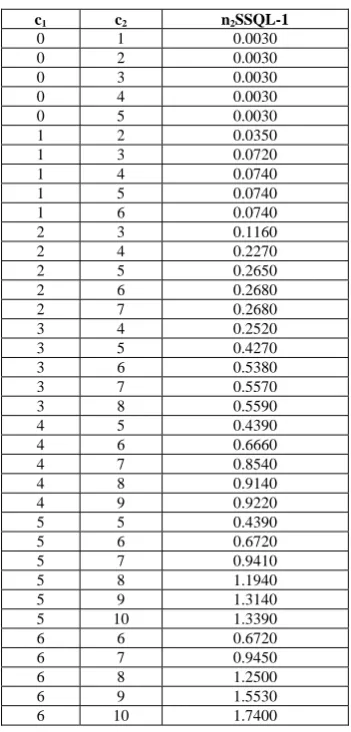
procedure given by [Schilling (1967)] is used for constructing the mixed sampling plan as attribute plan indexed through SSQL-1 [for β1" = (β1 – β1') / (1-β1')]. For the assumption β1=0.9999966 and β1'=0.50, the n2SSQL-1

values are calculated for different values of c1 and c2 using visual basic program and is presented in Table1.

The sigma level of the process is calculated using the Process Sigma Calculator by providing the sample size and acceptance number.

8.1 Selection of the plan

Table 1 is used to construct the plans when SSQL-1, c1, and c2 are given. For any given values of

SSQL-1, c1 and c2 one can determine n2 value using n2 = n2SSQL-1/SSQL-1.

8.2 Example

Given SSQL-1=0.00005, c1=1, c2=3and β1'=0.50, the value of n2SSQL-1 is selected from Table 1 as

0.0720 and the corresponding sample size n2 is computed as n2= n2SSQL-1/SSQL-1=0.0720/0.00005=1440

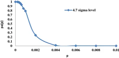
which is associated with 4.7 sigma level. For a fixed β1'=0.50, the Mixed Sampling Plan with Conditional

Repetitive Group Sampling Plan as attribute plan are n2=1440, c1=1 and c2=3 for a specified SSQL-1=0.00005.

8.3 Practical Application

Suppose the plan with n1 = 10, k = 1.5, c1=1 and c2=3 to be applied to the lot-by-lot acceptance

inspection of a Sanyo battery. The characteristic to be inspected is the “weight of a Sanyo battery in g” for which there is a specified upper limit of 46.5g with a known standard deviation (

σ

) of 0.02g. In this example, U = 46.5g,

σ

= 0.02g and k = 1.5. A = U - k

σ

= 46.5 – (1.5) (0.02) = 46.47g.

Now, by applying the variable inspection first, take a random sample of size n1=10 from the lot. Record

the sample results and find

X

. If

X

≤ A = U - k

σ

=46.47g, accept the lot otherwise take a random sample of size n2 =1440 and apply attribute inspection.

Under attribute inspection, the Conditional Repetitive Group Sampling Plan as attribute plan, if the manufacturer fixes the values β1'=0.50, SSQL-1=0.00005 (5 non-conformities out of 1 lakh batteries) then

select a sample of 1440 batteries, and count the number of non-conformities (d). If the weight of any battery is greater than 46.5g, then it is termed as defective. If the number of non-conformities d ≤ 1, accept the lot and if d >3 reject the lot and inform the management to improve the quality. If 1<d≤ 3, then the current lot of batteries is accepted if the preceding ‘i’ (i = 1) lot shows d ≤ 1 in the sample of batteries, otherwise reject the batteries and inform the management for quality improvement. The OC curve of the plan in Example 8.2 is presented in the Figure 1.

0 0.1 0.2 0.3 0.4 0.5 0.6 0.7 0.8 0.9 1

0 0.002 0.004 0.006 0.008 0.01

pa

(p

)

p

4.7 sigma level

9. Construction of MSP with Conditional Repetitive Group Sampling Plan as attribute plan indexed through SSQL-2

In this section the mixed sampling plan indexed through SSQL-2 is constructed. A point on the OC curve can be fixed such that the probability of acceptance of fraction defective SSQL-2 isβ2. The general

procedure given by Schilling (1967) is used for constructing the mixed sampling plan as attribute plan indexed through SSQL-2 [for β2" = (β2 – β2') / (1-β2')]. For the assumption β2 = 0.0000068 and β2' = 0.0000034, the

n2SSQL-2 values are calculated for different values c1 and c2 using visual basic program and is presented in

Table2.

9.1 Example

Given SSQL-2=0.008, c1=1, c2=2 and β1'=0.50, the value of n2SSQL-2 is selected from Table 1 as

15.3890 and the corresponding sample size n2 is computed as n2= n2SSQL-2/SSQL-2=15.3890/0.008=1924

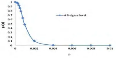
which is associated with 4.8 sigma level. For a fixed β1'=0.50, the Mixed Sampling Plan with Conditional

Repetitive Group Sampling Plan as attribute plan are n2=1924, c1=1 and c2=2 for a specified SSQL-1=0.008.

9.2 Practical Application

Suppose the plan with n1 = 10, k = 1.5, c1=1 and c2=2 to be applied to the lot-by-lot acceptance

inspection of a Laptop AC Adapter. The characteristic to be inspected is the “super slim of a Laptop AC Adapter in cm” for which there is a specified upper limit of 1.65cm with a known standard deviation (

σ

) of 0.02mm. In this example, U = 1.65cm,

σ

= 0.02cm and k = 1.5. A = U - k

σ

= 1.65 – (1.5) (0.02) = 1.62cm.

Now, by applying the variable inspection first, take a random sample of size n1=10 from the lot. Record

the sample results and find

X

. If

X

≤ A = U - k

σ

=1.62cm, accept the lot otherwise take a random sample of size n2 =1924 and apply attribute inspection.

Under attribute inspection, the Conditional Repetitive Group Sampling Plan as attribute plan, if the distributor fixes the values β1'=0.50, SSQL-1=0.008 (8 non-conformities out of 1 thousand) then select a sample

of 1924 adapters, and count the number of non-conformities (d). If the slim of any adapter is greater than 1.65cm, then it is termed as defective. If the number of non-conformities d ≤ 1, accept the lot and if d >2 reject the lot and inform the management to improve the quality. If 1<d≤ 2, then the current lot of adapters is accepted if the preceding ‘i’ (i = 1) lot shows d ≤ 1 in the sample adapters, otherwise reject the batteries and inform the management for quality improvement. The OC curve of the plan in Example 9.1 is presented in the Figure 2.

Fig. 2. OC curve for the plan n2=1924, c1=1 and c2=2

Conclusion:

References

[1] Bowker, A. H.; Goode, H.P. (1952): Sampling Inspection by Variables. McGraw Hill, New York.

[2] Dodge, (1932): Statistical control in sampling Inspection. American Mechanist. Oct 1932: 1085-88. Nov 1932, : 1129-31. [3] Dodge,; Roming,; (1942): Army service forces tables, Bell telephone laboratories, United States.

[4] Govindaraju, K.; (1987): An interesting observations in Acceptance Sampling. Economic Quality Control Journal, 2(4), pp.89-92. [5] Radhakrishnan, R. (2009): Construction of Six Sigma based Sampling Plans. Post Doctoral Thesis (D.Sc), submitted to Bharathiar

University, Tamilnadu, India.

[6] Radhakrishnan, R..; Glorypersial, J. (2011a): Construction of Mixed Sampling Plans Indexed through Six Sigma Quality Levels with Double Sampling Plan as Attribute Plan as Attribute Plan. International Journal of Statistics and Analysis, 1(1), pp.1-10.

[7] Radhakrishnan, R..; Glorypersial, J. (2011b): Construction of Mixed Sampling Plans Indexed through Six Sigma Quality Levels with Conditional Double Sampling Plan as Attribute Plan. International Journal of Recent Scientific Research, 2(7), pp. 232-236.

[8] Radhakrishnan, R..; Glorypersial, J. (2011c): Construction of Mixed Sampling Plans Indexed through Six Sigma Quality Levels with Chain Sampling Plan – (0,1) as Attribute Plan, International Journals of Multi Disciplinary Research Academy, ISSN 2249-0558, 1(6), pp.179-199.

[9] Radhakrishnan, R.; Sivakumaran, P.K. (2008): Construction and Selection of Six Sigma Sampling Plan indexed through Six Sigma Quality Level. International Journal of Statistics and Systems, 3(2), pp.153-159.

[10] Radhakrishnan, R.; Sivakumaran, P.K. (2009): Selection of Conditional Repetitive Group Sampling Plans indexed through Six Sigma Quality Levels. International Journal of Statistics and Management System (IJSMS).

[11] Radhakrishnan, R.; Sampath Kumar, R..; Saravanan, P.G. (2009): Construction of Dependent Mixed Sampling Plan using Single Sampling Plan as attribute plan. The International Journal of Statistics and Systems, 4(1), ISSN 0973-2675, pp:67-74.

[12] Radhakrishanan, R.; Saravanan, P.G.S. (2010); Construction of dependent Mixed Sampling Plans using Chain Sampling Plan of type ChSP-1 indexed through AQL. National Journal of Technology, 6(4), ISSN 0973-1334, pp:37-41.

[13] Romboski, L.D. (1969): An Investigation of Quick Switching Acceptance Sampling System. Ph.D Thesis, Rutgers- the state University, New Brunswick, New Jersey.

[14] Sampathkumar, R. (2007): Construction and Selection of Mixed variables Attributes Sampling Plans. Ph.D thesis, Bharathiar University, Tamilnadu, India.

[15] Sekkizhar, J. (2007): Designing of sampling plans using Intervened Random effect Poisson distribution, Ph.D. Thesis, Bharathiar University, Coimbatore, India.

[16] Schilling, E.G. (1967): A general method for determining the operating characteristics of mixed variables. Attribute sampling Plans single side specifications, S.D known, Ph.D thesis Rutgers, The State University, New Brunswick, New Jersy. [17] Shankar, G. ; Mohapatra, B.N. (1993): GERT Analysis of Conditional Repetitive Group Sampling Plan. International Journal of

Quality and Reliability Management, 10(2), pp.50-62.

[18] Sherman, R.E. (1965): Design and Evaluation of a Repetitive Group Sampling Plan. Technometrics, 10(1), pp.11-21.

[19] Soundararajan, V.; Ramasamy, V. (1984): Designing Repetitive Group Sampling Plan indexed by AQL and LQL. IAPQR Transaction, 9(1), pp.9-14.

[20] Soundararajan, V.; Ramasamy, V. (1986): Procedures and Tables for Construction and selection of Repetitive Group Sampling (RGS) plan. The QR journal, 13(13), pp.14-21.

[21] Wortham, A.W.; Mogg, J.M. (1970): Dependent Stage Sampling Inspection. The International Journal of Production and Research, 8(4), pp.385-395.

[22] Motorola: http://www.motorola.com/

Table 1: Various characteristics of the MSP when (SSQL-1, β1) is known with β1 = 0.9999966, β1' = 0.50.

c1 c2 n2SSQL-1

0 1 0.0030

0 2 0.0030

0 3 0.0030

0 4 0.0030

0 5 0.0030

1 2 0.0350

1 3 0.0720

1 4 0.0740

1 5 0.0740

1 6 0.0740

2 3 0.1160

2 4 0.2270

2 5 0.2650

2 6 0.2680

2 7 0.2680

3 4 0.2520

3 5 0.4270

3 6 0.5380

3 7 0.5570

3 8 0.5590

4 5 0.4390

4 6 0.6660

4 7 0.8540

4 8 0.9140

4 9 0.9220

5 5 0.4390

5 6 0.6720

5 7 0.9410

5 8 1.1940

5 9 1.3140

5 10 1.3390

6 6 0.6720

6 7 0.9450

6 8 1.2500

6 9 1.5530

Table2: Various characteristics of the MSP when (SSQL-2, β2) is known with β2 = 0.0000068 and β2' = 0.0000034.

c1 c2 n2SSQL-2

0 1 12.5920

0 2 12.5920

0 3 12.5920

0 4 12.5920

0 5 12.5920

1 2 15.3890

1 3 15.3890

1 4 15.3890

1 5 15.3890

1 6 15.3890

2 3 17.7660

2 4 17.7660

2 5 17.7660

2 6 17.7660

2 7 17.7660

3 4 19.9310

3 5 19.9310

3 6 19.9310

3 7 19.9310

3 8 19.9310

4 5 21.9610

4 6 21.9610

4 7 21.9610

4 8 21.9610

4 9 21.9610

5 5 23.8950

5 6 23.8950

5 7 23.8950

5 8 23.8950

5 9 23.8950

5 10 23.8950

6 6 25.7570

6 7 25.7570

6 8 25.7570

6 9 25.7570