https://doi.org/10.5194/amt-11-6539-2018 © Author(s) 2018. This work is distributed under the Creative Commons Attribution 4.0 License.
Improved retrievals of carbon dioxide from Orbiting Carbon
Observatory-2 with the version 8 ACOS algorithm
Christopher W. O’Dell1, Annmarie Eldering2, Paul O. Wennberg3, David Crisp2, Michael R. Gunson2, Brendan Fisher2, Christian Frankenberg3, Matthäus Kiel3, Hannakaisa Lindqvist4, Lukas Mandrake2,
Aronne Merrelli5, Vijay Natraj2, Robert R. Nelson1, Gregory B. Osterman2, Vivienne H. Payne2, Thomas E. Taylor1, Debra Wunch6, Brian J. Drouin2, Fabiano Oyafuso2, Albert Chang2, James McDuffie2, Michael Smyth2,
David F. Baker1, Sourish Basu7,8, Frédéric Chevallier9, Sean M. R. Crowell10, Liang Feng11,12, Paul I. Palmer11,12, Mavendra Dubey13, Omaira E. García14, David W. T. Griffith15, Frank Hase16, Laura T. Iraci17, Rigel Kivi18, Isamu Morino19, Justus Notholt20, Hirofumi Ohyama19, Christof Petri20, Coleen M. Roehl3, Mahesh K. Sha21, Kimberly Strong6, Ralf Sussmann22, Yao Te23, Osamu Uchino19, and Voltaire A. Velazco15
1Cooperative Institute for Research in the Atmosphere, Colorado State University, Fort Collins, CO, USA 2Jet Propulsion Laboratory, California Institute of Technology, Pasadena, CA, USA
3Division of Geological and Planetary Sciences, California Institute of Technology, Pasadena, CA, USA 4Finnish Meteorological Institute, Helsinki, Finland
5SSEC, University of Wisconsin-Madison, Madison, WI, USA 6Department of Physics, University of Toronto, Toronto, Canada
7NOAA Earth System Research Laboratory, Global Monitoring Division, Boulder, CO, USA
8Cooperative Institute for Research in Environmental Sciences, University of Colorado Boulder, Boulder, Colorado, USA 9Laboratoire des Sciences du Climat et de l’Environnement, IPSL, CEA-CNRS-UVSQ, Gif-sur-Yvette, France
10College of Atmospheric and Geographic Sciences, University of Oklahoma, Norman, OK, USA 11National Centre for Earth Observation, University of Edinburgh, UK
12School of GeoSciences, University of Edinburgh, UK 13Los Alamos National Laboratory, Los Alamos, NM, USA
14Izaña Atmospheric Research Center, Meteorological State Agency of Spain (AEMet), Santa Cruz de Tenerife, Spain 15Centre for Atmospheric Chemistry, University of Wollongong, Wollongong, Australia
16Karlsruhe Institute of Technology, IMK-ASF, Karlsruhe, Germany 17NASA Ames Research Center, Moffett Field, CA, USA
18Finnish Meteorological Institute, Sodankylä, Finland
19National Institute for Environmental Studies (NIES), Tsukuba, Japan 20Institute of Environmental Physics, University of Bremen, Bremen, Germany 21Royal Belgian Institute for Space Aeronomy, Brussels, Belgium
22Karlsruhe Institute of Technology, IMK-IFU, Garmisch-Partenkirchen, Germany
23LERMA-IPSL, Sorbonne Université, Observatoire de Paris, Université PSL, CNRS, 75005, Paris, France
Correspondence:Christopher W. O’Dell ([email protected]) Received: 27 July 2018 – Discussion started: 16 August 2018
Abstract. Since September 2014, NASA’s Orbiting Carbon Observatory-2 (OCO-2) satellite has been taking measure-ments of reflected solar spectra and using them to infer at-mospheric carbon dioxide levels. This work provides details of the OCO-2 retrieval algorithm, versions 7 and 8, used to derive the column-averaged dry air mole fraction of atmo-spheric CO2(XCO2) for the roughly 100 000 cloud-free mea-surements recorded by OCO-2 each day. The algorithm is based on the Atmospheric Carbon Observations from Space (ACOS) algorithm which has been applied to observations from the Greenhouse Gases Observing SATellite (GOSAT) since 2009, with modifications necessary for OCO-2. Be-cause high accuracy, better than 0.25 %, is required in or-der to accurately infer carbon sources and sinks from XCO2, significant errors and regional-scale biases in the measure-ments must be minimized. We discuss efforts to filter out poor-quality measurements, and correct the remaining good-quality measurements to minimize regional-scale biases. Up-dates to the radiance calibration and retrieval forward model in version 8 have improved many aspects of the retrieved data products. The version 8 data appear to have reduced regional-scale biases overall, and demonstrate a clear improvement over the version 7 data. In particular, error variance with re-spect to TCCON was reduced by 20 % over land and 40 % over ocean between versions 7 and 8, and nadir and glint observations over land are now more consistent. While this paper documents the significant improvements in the ACOS algorithm, it will continue to evolve and improve as the CO2
data record continues to expand.
1 Introduction
Bias-free measurement of atmospheric CO2 concentrations
from space is a long-pursued goal in the carbon cycle com-munity. Such measurements are critical for inferring sources and sinks of carbon, and how these sources and sinks change over time due to both anthropogenic and natural causes (e.g., Rayner and O’Brien, 2001; Chevallier et al., 2007; Baker et al., 2010). The first instrument capable of CO2
measure-ments from space using the near- and short-wavelength in-frared was SCIAMACHY, the SCanning Imaging Absorp-tion spectroMeter for Atmospheric CHartographY (Buch-witz et al., 2005; Reuter et al., 2011), which operated from 2002 to 2012. This was followed by the first dedicated green-house gas satellite, the Japanese Greengreen-house gases Observ-ing SATellite (GOSAT), which launched in January 2009 (Yokota et al., 2009). The Orbiting Carbon Observatory-2 (OCO-2) followed on 2 July 2014, with the goal of measuring the column-averaged dry air mole fraction of carbon diox-ide (XCO2) with sufficient precision and accuracy to enable greatly enhanced understanding of the surface–atmosphere exchange of CO2on regional scales (Crisp et al., 2008; Crisp,
2015). OCO-2 was preceded by the original OCO mission,
which failed due to a launch vehicle malfunction in 2009. Retrieval algorithms originally developed for OCO (Con-nor et al., 2008) have been continuously refined since 2009 (O’Dell et al., 2012), by application to data from GOSAT.
XCO2 measurements from the OCO-2 version 7 data prod-uct (Eldering et al., 2017a) have recently been used to esti-mate CO2fluxes from both natural (Liu et al., 2017;
Chat-terjee et al., 2017; Crowell et al., 2018a) and anthropogenic (Hakkarainen et al., 2016; Schwandner et al., 2017; Nassar et al., 2017) sources; see Eldering et al. (2017b) for a com-plete review of these findings. However, XCO2 measurements must be both extremely accurate and precise in order to accu-rately determine fluxes (Miller et al., 2007), since fluxes are determined from small (<2.5 %) spatial and temporal gradi-ents in the XCO2 field. Spatially coherent biases in XCO2 on regional scales as small as a few tenths of a part-per-million (ppm) in XCO2 can lead to spurious values of inferred fluxes (Chevallier et al., 2014).
The ACOS algorithm was originally developed for OCO. It was first applied to GOSAT data in 2009 and has con-tinuously evolved and improved in the intervening years. Generally, good error statistics were shown for GOSAT ob-servations over both land and water, with typical biases below 1 ppm based on comparisons to both ground-based (Lindqvist et al., 2015; Kulawik et al., 2016) and aircraft (Frankenberg et al., 2016) validation data. After the success-ful launch of OCO-2, the ACOS algorithm was further mod-ified and tuned for application to the OCO-2 spectra. XCO2 error statistics are similar to those from GOSAT, with rms er-rors less than 1.5 ppm when compared against most ground-based Total Carbon Column Observing Network (TCCON, Wunch et al., 2010) stations (Wunch et al., 2017). How-ever, Wunch et al. (2017) noted that important biases re-main, in particular related to latitude, surface properties, and atmospheric scattering by clouds and aerosols. A particu-larly troubling bias evident in the Southern Hemisphere mid-latitude ocean in austral winter had amplitudes as large as several ppm. This bias was not seen in ACOS retrievals using GOSAT data, though GOSAT’s ocean glint viewing geome-try was restricted and could not typically see this far south, potentially masking the problem.
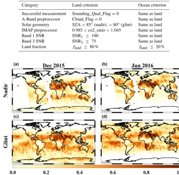
Table 1.Prescreening filter criteria.
Category Land criterion Ocean criterion
Successful measurement Sounding_Qual_Flag=0 Same as land A-Band preprocessor Cloud_Flag=0 Same as land Solar geometry SZA<85◦(nadir),<80◦(glint) Same as land IMAP preprocessor 0.985<co2_ratio<1.045 Same as land
Band 1 SNR SNR1 ≥ 100 Same as land
Band 3 SNR SNR3 ≥ 75 Same as land
Land fraction fland ≥ 80 % fland ≤ 20 %
Figure 1.Fraction of soundings passing the OCO-2 B8 prescreening filter in December 2015(a, c)and June 2016(b, d), for both nadir mode(a, b)and glint mode(c, d). Starting in November 2015, about one-third of all orbits are performed in nadir mode, and two-thirds are performed in glint mode.
versions 7 and 8, and the discussion in Sect. 6 concludes the paper.
2 Data and prescreening
Because only scenes with sufficient signal and nearly de-void of cloud and aerosol contamination can yield success-ful XCO2 retrievals, a prescreener is used for OCO-2 sound-ings before processing by the Level-2 “Full-Physics” (L2FP) XCO2 retrieval algorithm. Our prescreening module requires outputs from two fast algorithms, described in detail in Tay-lor et al. (2016). First, the “A-band Preprocessor” (ABP) per-forms a fast retrieval of surface pressure using the O2A band
only, assuming that no clouds or aerosols are present. Poor spectral fits and differences between the retrieved anda pri-orisurface pressure greater than 25 hPa are used to identify the presence of cloud or aerosol contamination. Scenes
with-out sufficient signal to noise in the O2A band are skipped
al-together. Second, the “IMAP-DOAS” preprocessor performs fast, clear-sky fits to the weak and strong CO2bands at 1.61
and 2.06 µm, respectively. While this preprocessor solves for a number of variables, the CO2and H2O columns, which are
fit independently of each of these two bands, are most rele-vant for cloud screening. From these spectral fits, the strong-to-weak ratios of the column-integrated CO2 and H2O are
derived. The CO2ratio must be within a certain range (near
unity) for the scene to be deemed sufficiently clear to warrant a Full-Physics retrieval. Other screens are used to remove soundings unlikely to yield successful XCO2, such as those at high solar zenith angle or for which the continuum SNR lev-els are too low. Unlike in version 7 of the OCO-2 algorithm, there is no explicit screen for snow- and ice-covered surfaces. However, the surface albedo in the strong CO2band is low
filter will remove many of those scenes. The full prescreen-ing criteria for OCO-2 B8 are given in Table 1.
In total, roughly 26 % of land soundings pass our pre-screener (28 % land nadir, 25 % land glint) and 27 % of ocean glint soundings pass it as well. Generally these fractions are strong functions of both location and time of year. To illus-trate this, the fractions of soundings passing the prescreen-ing criteria for December 2015 and June 2016 are shown in Fig. 1. A number of features are observed. A higher frac-tion of soundings are passed in the tropics than at higher lati-tudes relative to the sub-solar latitude (∼ −23◦in December and+23◦in June), and the passing rates tend to be higher over bright versus dark surfaces. Also, few soundings survive over the tropical rainforests in South America and Africa, which are often cloudy. A significant number of soundings survive prescreening over the Greenland and Antarctic ice sheets during their summer season (this was not the case in version 7), though it is shown later that most of these fail the post-retrieval quality screening (Sect. 4.2). About 10 % of nadir soundings over ocean pass the prescreening criteria; this occurs in regions where the nadir view is relatively close to the glint geometry, typically near the sub-solar latitude. These nadir ocean soundings are currently removed by post-retrieval filtering, as their quality relative to the glint ocean observations has not yet been evaluated. A final obvious fea-ture is that fewer soundings are available in nadir mode than in glint – this is because many orbits over the Atlantic and Pacific oceans became “full-time” glint-mode orbits begin-ning in November 2015 (Crisp et al., 2017). Prior to that, there were equal numbers of nadir and glint orbits, but after that change, approximately one-third of all orbits are nadir and two-thirds are glint.
3 The NASA ACOS XCO2 retrieval algorithm as applied to OCO-2
The original ACOS XCO2 retrieval algorithm over land (ver-sion 2.9) was described in O’Dell et al. (2012), with details specific to GOSAT given in Crisp et al. (2012). Details of the spectroscopy used at that time were published in Thompson et al. (2012). In this section, we give an overview of the evo-lution from ACOS version 2.9 to OCO-2 versions 7 and 8, including spectroscopy, aerosol treatment, and a number of other changes.
Briefly, the NASA ACOS algorithm uses optimal estima-tion to solve for parameters of a state vector to obtain the best match to spectra from the three GOSAT or OCO-2 near-infrared bands and consistent with a prior constraint. These bands are the O2A band at 0.76 µm (band 1), the weak CO2
band at 1.61 µm (band 2), and the strong CO2band at 2.06 µm
(band 3). The state vector parameters, listed in Table 2, in-clude the profile of CO2at twenty atmospheric levels along
with a number of ancillary parameters to which the GOSAT and OCO-2 near-infrared spectra are sensitive. These include
surface pressure, surface albedo parameters (over land only), a temperature profile offset and water vapor profile multi-plier, and parameters related to the wavelength scale of the spectra (dispersion shift and stretch). The latter are relative to the preflight values of these parameters, described in Lee et al. (2017). Because telluric line positions are known with high accuracy, the retrieval solves for them with virtually no dependence on the prior. To account for scattering effects of thin cloud or aerosol, the retrieval also solves simultaneously for amounts and Gaussian vertical profiles (as described in Sect. 3.1) of five different kinds of scatterers with fixed opti-cal properties: a water cloud type, an ice cloud type, two fixed aerosol types, and beginning in version 8, an Upper Tropo-spheric/Lower Stratospheric (UTLS) sulfate aerosol layer. In addition, the retrieval also fits scaling factors for three spec-tral patterns per band, to account for imperfections in the spectroscopy, solar model, and instrument model, and deter-mined using singular value decomposition of our fit residu-als run on clear-sky soundings (Sect. 3.3). For solar-induced fluorescence (SIF) emission from plants on land, we fit for two SIF parameters which are needed to account for this flu-orescence in the L2 spectra (Sect. 3.5). These SIF parame-ters are not the official SIF data product; that product is de-rived from the IMAP prescreener through a dedicated fit (Sun et al., 2018). In total, there are typically 55 fitted parameters for land retrievals and 53 for ocean1. With the exception of CO2, thea prioricovariance matrix is diagonal, with the 1σ
uncertainties as given in Table 2.
The first documented algorithm version, B2.9 as described in O’Dell et al. (2012), had several deficiencies which occa-sionally produced large biases in the retrieved XCO2 (Wunch et al., 2011a). This early version of the algorithm also con-tained some cumbersome traits, such as a variable number of vertical levels from sounding to sounding, which made the output difficult to use. The observed XCO2 biases were par-tially related to the aerosol parameterization, demonstrated by the fact that clear-sky retrievals of clear-sky simulations did not exhibit substantial biases (O’Dell et al., 2012). Fur-thermore, errors in the O2and CO2spectroscopy were
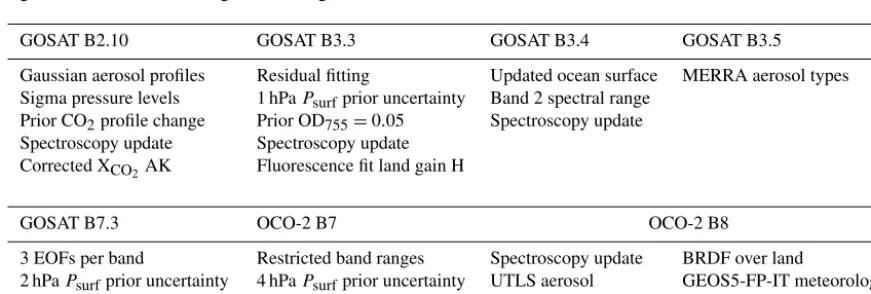
sus-pected to be an additional source of bias. Over the course of several years, a number of changes to the algorithm were therefore implemented to yield the present version, B8. The changes are too numerous to fully describe here, but the most important ones are listed in Table 3. The changes fall into several major categories, with spectroscopy, aerosol treat-ment, treatment of the ocean surface, and chlorophyll fluo-rescence being the most important. In B8, the meteorology used to prescribe the a priori temperature profile, water vapor profile, and surface pressure was also changed (Sect. 3.5).
Further, as listed in Table 4, some minor retrieval differ-ences exist between the GOSAT and OCO-2 versions of the algorithm. Besides using instrument models specific to each
1This excludes parameters in our state vector with prior
Table 2.General setup of the ACOS state vector.
Element No. of elements Prior value Prior uncertainty (1σ) Notes
CO2values 20 Same as TCCON Same as ACOS B2.9 Defined on sigma pressure levels
Temperature offset 1 0 K 5 K Rel. to prior profile
Surface pressure 1 From prior meteorology 4 hPa Prior unc. 1 hPa for B3.5
H2O scale factor 1 1.0 0.5 Multiplier on prior profile
Aerosol type 1,2 OD755 2 From MERRA ±factor of 7.39 Water, ice cloud OD755 2 0.0125 ±factor of 6.05
Aerosol type 1,2x0 2 0.9 0.2
Water cloudx0 1 0.75 0.4
Ice cloudx0 1 Just below tropopause 0.2
Aerosol type 1,2σa 2 0.05 0.01
Water cloudσa 1 0.1 0.01
Ice cloudσa 1 0.04 0.01
UTLS aerosol OD755 1 0.006 ±factor of 6.05 Introduced in B8
Albedo mean land 1 per band Prior calc. 1.0 Land
Albedo slope land 1 per band 0.0 0.0005 Land; units of 1/cm−1
Albedo mean ocean 1 per band 0.02 {0.2,0.2,1e−3} Ocean
Albedo slope ocean 1 per band 0.0 1.0 Ocean; units of 1/cm−1
SIF mean 1 Prior calc. 0.008 Land
SIF slope 1 0.0018 0.0007 Land; units of 1/cm−1
Wind speed 1 From prior meteorology 5 m s−1 Ocean
Dispersion shift 1 per band 0.0 0.4 of channel FWHM
Dispersion stretch 1 per band 0.0 1 pm/channel OCO-2 only
EOF amplitudes 3 per band 0.0 10.0 1 per band for B3.5 & earlier
Table 3.Significant ACOS retrieval algorithm changes.
GOSAT B2.10 GOSAT B3.3 GOSAT B3.4 GOSAT B3.5
Gaussian aerosol profiles Residual fitting Updated ocean surface MERRA aerosol types Sigma pressure levels 1 hPaPsurfprior uncertainty Band 2 spectral range
Prior CO2profile change Prior OD755=0.05 Spectroscopy update
Spectroscopy update Spectroscopy update Corrected XCO2AK Fluorescence fit land gain H
GOSAT B7.3 OCO-2 B7 OCO-2 B8
3 EOFs per band Restricted band ranges Spectroscopy update BRDF over land
2 hPaPsurfprior uncertainty 4 hPaPsurfprior uncertainty UTLS aerosol GEOS5-FP-IT meteorology
Updated cloud ice properties L1B improvements Numerous small changes
instrument (such as wavelengths of the various channels, noise model, and instrument line shape functions), slightly different spectral ranges are fit for each instrument. Gener-ally, this is because the trusted calibrated range of OCO-2 spectra is slightly smaller than that of GOSAT, due to the dif-ferences in design of the OCO-2 grating spectrometer versus the GOSAT Fourier transform spectrometers. Additionally, while all channels in each band in the given spectral ranges are used for GOSAT, some band channels are masked out for OCO-2. This is due to either underlying bad pixels in the detector arrays or to transient cosmic rays that induce
tem-porary spurious readings in random channels. Both of these processes are described in detail in Crisp et al. (2017). 3.1 Aerosol-related changes
Table 4.ACOS retrieval differences between GOSAT and OCO-2.
Category GOSAT OCO-2
Radiance used Estimated total intensity OCO-2 single polarization EOFs, band ranges Wavenumber space Channel space
Fit O2A band offset ? Yes No
SIF prior 0 From IMAP retrieval
Per-band dispersion parameters Offset only Offset, slope Band 1 fitted range 758.1–772.2 nm 759.2–771.5 nm Band 2 fitted range 1597.4–1618.1 nm 1598.1–1617.9 nm Band 3 fitted range 2042.1–2079.0 nm 2047.8–2079.9 nm
Channel mask None Bad samples, spikes
the surface pressure. Therefore,xranges from zero at the top of the atmosphere to one at the surface. The functional form is simply
ρaer(x)=Cexp
−(x−x0) 2
2σ2 a
, (1)
where for each aerosol typex0is the vertical location at peak
aerosol density andσais the Gaussian 1σprofile width. Both
of the latter variables are specified in units of relative pres-sure x. The prefactor C is defined such that the aerosol or cloud optical depth at 755 nm, hereafter OD755, equals the
desired value. In the retrieval algorithm, the fitted quanti-ties are ln OD755and peak heightpr,0for each aerosol type,
with the exception of the stratospheric aerosol (described in Sect. 3.1.1) for which only the optical depth is retrieved. Be-cause it has been shown that GOSAT and OCO-2-like spec-tra have little sensitivity to the Gaussian profile width (Butz et al., 2009), this parameter is fixed in both the GOSAT and OCO-2 retrievals for all particle types. The prior profiles for each fitted type are shown in Fig. 2.
The change to a sigma-level pressure system was incorpo-rated at about the same time as the shift to Gaussian aerosol profiles. Instead of fixed pressure levels, the pressure levels scale with the surface pressure:
pi=ai psurf, (2)
where theaiare chosen such that the total number of pressure
boundaries is 20, and the layers have roughly equal pressure widths. The top-most model level is set to 0.01 hPa.
The optical properties of the four scattering types re-mained unchanged from versions B2.9 to B3.4 and are de-scribed in O’Dell et al. (2012). However, the use of two fixed aerosol types, types “2b” and “3b” from the Kahn et al. (2001) climatology, did not accurately represent the true global variability of aerosol on the length scales and timescales probed by GOSAT and OCO-2. Beginning with build 3.5, the aerosol types were changed to be location- and time-dependent, with the prior type information coming from the aerosol climatology of the Modern-Era Retrospective analysis for Research and Applications (MERRA, Rienecker
Figure 2.Prior Gaussian profiles of the lower tropospheric aerosol types (red), water cloud (blue), ice cloud (purple), and stratospheric aerosol (green). The local aerosol optical depth (AOD) per unit pres-sure at 755 nm is plotted as a function of the relative prespres-sure. The lower tropospheric aerosol prior optical depth is not fixed as for the other types, but rather is taken from a climatology described in the text.
Figure 3.Optical properties of aerosols and clouds used in the L2FP code as a function of wavelength.(a)Extinction efficiency relative to that at 755 nm.(b)Single scattering albedo.(c)Asymmetry parameter. DU: dust, SS: sea salt, BC: black carbon, OC: organic carbon, SO: sulfate, WC: water cloud, IC: ice cloud. The spectral ranges of the three OCO-2 bands are demarcated by the dashed vertical lines.
organic carbon (BC and OC, respectively). Dust and sea salt are each tracked in five separate size bins. Organic carbon and black carbon are tracked in both hydrophobic and hy-drophilic categories. In addition to the carbonaceous types, sulfate aerosol and sea salt are also hydrophilic and hence have optical properties that depend on the local relative hu-midity (RH).
For the aerosol prior in the ACOS retrieval, we primarily sought to specify the typical dominant aerosol types present (in terms of their contribution to the optical depth in the OCO-2 bands) in a given location at a given time of year. Monthly aerosol fields were derived from the MERRA model for the year 2010, and are used for all years in the ACOS re-trieval. We aggregated the 15 MERRA types, eight of which have RH-dependent optical properties, into the five aggre-gated types listed above. We used typical density weightings and relative humidity values to create the optical properties for these aggregated types, as described in Crisp et al. (2017). Their optical properties, including extinction efficiency, sin-gle scattering albedo, and asymmetry parameter, are shown in Fig. 3. The organic carbon and sulfate aerosol are gen-erally similar in their optical properties, though their single scattering albedos diverge somewhat in the CO2bands. The
sea salt, water cloud, and dust optical properties are relatively similar across the OCO-2 spectral range.
At each sounding location, the two aggregated aerosol types with the highest mean monthly values of the OD755
are selected to be retrieved by the L2FP algorithm. In pre-vious algorithm versions, the total prior OD755 was set to
0.15, apportioned equally among four scattering types (water cloud, ice cloud, and two tropospheric aerosol types). How-ever, it was found this was generally too high to allow a fit near OD755=0 for scenes that were almost entirely free of
aerosol. This “clear-sky bias” was seen in early simulation
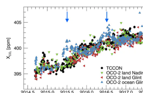
Figure 4.Comparison of XCO2time series for OCO-2 version 7 and TCCON, over several years at the station in Wollongong, Australia (Griffith et al., 2014b). Each OCO-2 symbol represents an overpass average. A simple geometric colocation strategy was used in which OCO-2 soundings within±7.5◦latitude and±30◦longitude of the TCCON station were retained. Large positive biases occur in the ocean glint soundings in the Southern Hemisphere winter (blue ar-rows). As seen in Fig. 19, these large biases primarily occur in the southern oceans.
tests (O’Dell et al., 2012). The prior OD755 is now set to
0.0125 for each cloud type, and set from the MERRA aerosol climatology for each tropospheric aerosol type as the average OD755of that type (at a particular location and month). There
is some evidence that the tropospheric aerosol priors are oc-casionally still too high; methods for specifying the aerosol prior are a continuing topic of investigation.
cloud ice model considered an ensemble of size-dependent non-spherical ice crystal habits in random orientation. As ice crystal surface roughness was later shown to significantly af-fect scattering by ice crystals, and simulations with rough-ened model particles were more consistent with satellite ob-servations of ice cloud polarized reflectances (Yang et al., 2013), we updated the cloud ice optical properties to cor-respond to the MODIS Collection 6 model, which describes scattering by severely roughened hexagonal column ice crys-tal aggregates (Baum et al., 2014). This update also fixed sev-eral minor issues in the previous cloud ice model, such as those resulting from linear interpolation of the optical prop-erties from MODIS wavelength bands to OCO-2, and those relating to truncation of the phase function.
3.1.1 The need for a stratospheric aerosol
When validating version 7 XCO2 retrievals, it was discov-ered via comparisons to both TCCON and models that most ocean soundings in the most southerly∼10 degrees of lati-tude exhibited a high bias of 1–3 ppm during the austral win-ter (Wunch et al., 2017). Figure 4 shows the bias appears in the Southern Hemisphere winter over the Wollongong TC-CON station. The bias is seen in soundings over ocean but not land. The bias is also apparent relative to the Lauder TCCON station (Figs. 11 and A1 from Wunch et al., 2017). Compar-isons of OCO-2 soundings to models (Fig. 19) show the bias as a quasi-zonal band over the Southern Hemisphere oceans, again with the larger bias occurring in the Southern Hemi-sphere winter. There is also evidence of a similar but weaker band of high bias in the Northern Hemisphere. For 2015, it was hypothesized that small aerosol particles may have been injected into the UTLS by the explosive eruptions of the Cal-buco (22–30 April 2015) and Wolf (late May 2015) volcanos in southern–central Chile and the Galapagos Islands, respec-tively. The presence of an aerosol layer with visible optical depths around 0.01 was later confirmed with observations from the Cloud-Aerosol Lidar and Infrared Pathfinder Satel-lite Observatory (CALIPSO) and the Ozone Mapping Profile Suite (OMPS) satellites (Bègue et al., 2017). These optical depths are small, but have a large impact on the radiances, especially in the O2A band, due to their high altitude.
It was recognized that our version 7 retrieval algorithm had no way to accommodate the spectral signature of small stratospheric aerosol particles, which have a significantly larger effect on the O2A band than either of the CO2bands
due to the small size parameter, i.e, the ratio of the size of the scattering particle to the spectral wavelength. The spec-tral signature would essentially appear as a radiance offset in the O2A band. As a first test, we ran hundreds of retrievals
on a single sounding that had a large positive bias in the op-erational retrieval, using slightly different first-guess values for each retrieval. Essentially, a continuum of solutions was found (Fig. 5). On one end of retrieval space, an approxi-mately correct value of surface pressure was found by
in-Figure 5.Results of several hundred retrievals of a single ocean glint sounding (28.5◦S, 52.3◦W) measured on 26 June 2015. Each retrieval is identical except that each has a different first guess state, consistent with the prior uncertainty distribution. The retrieved rela-tive sulfate height (0=top-of-atmosphere; 1=surface) is shown on the ordinate, the reducedχ2from the strong (2.06 µm) CO2band
re-trieval is shown on the abscissa, and the retrieved XCO2is indicated by color. For reference, the result from the operational retrieval (ver-sion 7) is shown as the large filled circle. When the retrieval places the sulfate near the surface, as in the version 7 case, both the strong CO2bandχ2value and XCO2 tend to be higher. Conversely, when the retrieval pushes the sulfate closer to the top-of-atmosphere, the strong CO2bandχ2values and XCO2 tend toward lower values, a result that is more physically plausible.
serting a thicker ice cloud, which contains larger particles starting in the stratosphere, and therefore has a strong effect on all three bands (see Fig. 3). This type of solution pro-duced a poorχ2in the strong CO2band, typically>2. On
the other end of the continuum were solutions where the sul-fate layer, which was placed near the surface in the prior, was moved high up into the atmosphere. This solution regime had a much lower reducedχ2 (around 1.5) in the strong CO2
band and an XCO2 that was typically 3–4 ppm lower, and much more in line with TCCON and model estimates. In these cases, the amount of upper atmosphere cloud ice re-trieved was also reduced, as its role was taken over by the sulfate.
These tests indicated that a more realistic solution would often be found if the retrieval could push the prior sulfate into the upper atmosphere, though this seldom occurred. The amount of sulfate needed in the upper atmosphere in these cases is small, approximately 0.01 optical depth at 755 nm. That value is consistent with other observations (Bègue et al., 2017). In addition to actual small particles in the UTLS, the OCO-2 instrument has a documented problem which pro-duces a similar impact on the O2A and spectrum. As
of ice appears to build up on the OCO-2 Focal Plane Ar-rays (FPAs) over time. As this ice layer grows to a thick-ness similar to the anti-reflective coating thickthick-ness (tens of nanometers), it enhances the surface reflectance on the O2A
band FPA, producing a scattered light contribution of 0.1 to 0.2 %. Much smaller effects are seen on the CO2detectors.
The ice layer is sublimed off every 3–6 months when the instrument goes through a decontamination cycle. While at-tempts have been made to remove this scattered light con-tribution in the version 8 calibrated radiance (L1B) product, it is likely that some residual signal remains. Because this is primarily a radiance offset in the O2A band alone, it
pro-duces a signal similar to a small UTLS aerosol, and hence would also be mitigated by including a stratospheric aerosol in the retrieval. During algorithm testing of the stratospheric aerosol using version 7 L1B radiances (which contained the scattered light signature), we found that the amount of UTLS aerosol retrieved indeed correlated with the decontamination cycles, lending credence to this hypothesis.
Thus, in version 8 an additional sulfate aerosol was in-cluded in the retrieval state vector. For simplicity, a sulfate type identical to the lower-atmosphere type in terms of op-tical properties was used. Only the total opop-tical depth of the stratospheric sulfate is retrieved, while its Gaussian height and width are kept fixed. This solution treats both actual small particles in the UTLS as well as the radiometric offsets that accompany the real O2A band scattered light signal. Our
testing of the version 8 algorithm showed that including this state vector element not only reduced the Southern Ocean bias, but also reduced the negative tropical ocean bias and positive bias over higher northern-latitude lands that were also apparent in Fig. 19. A more complete comparison of ver-sion 7 and verver-sion 8 validation statistics is given in Sect. 5. 3.2 Spectroscopy-related changes
There have been substantial changes between the molecular cross sections used in the earliest ACOS versions and those used in B8. We continue to use in-house lookup tables of ab-sorption coefficients (ABSCO) parameterized as a function of temperature, pressure, wavelength, and water vapor mix-ing ratio for each of the main absorbmix-ing gases in the OCO-2 bands: O2, CO2, and water vapor (H2O). Successive versions
of these tables have been refined by incorporating new lab-oratory results and theoretical models for increasingly accu-rate absorption coefficients. The ABSCO version used in the B8 algorithm is ABSCO v5.0 (Drouin et al., 2017; Oyafuso et al., 2017); B7 used the previous ABSCO version, v4.2.
The ABSCO v5.0 O2A band tables represent a major step
forward from previous ABSCO versions. Earlier ABSCO versions integrated the highest-quality spectroscopic input from a range of studies that had focused on fitting differ-ent parameters independdiffer-ently. (See, for example, Thompson et al., 2012, and references therein.) The ABSCO v5.0 tables are based on self-consistent multispectral fits to laboratory
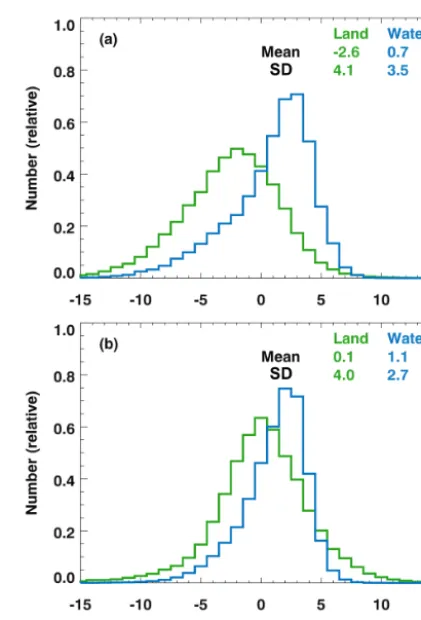
Figure 6.Retrieved minus prior surface pressure for a large selec-tion of OCO-2 soundings, using the oxygen-A band spectroscopy model from both(a)ABSCO v4.2 and (b)ABSCO v5.0, as de-scribed in the text. ABSCO v5.0 spectroscopy leads to a more con-sistent retrieval of surface pressure over both land and ocean sur-faces.
spectra that include line mixing, speed-dependent Voigt line shape parameters, and collision-induced absorption (CIA). This self-consistency, and the use of laboratory spectra cov-ering a range of pressures, temperatures, and measurement techniques, are key features of the approach. The O2spectral
line parameters, line mixing, and CIA used in ABSCO v5.0 are described in Drouin et al. (2017). Parameters for broaden-ing of O2by H2O are from the study by Drouin et al. (2014).
The impact of the latest multi-spectrum fitting update in the O2A band is shown in terms of the accuracy of the
trieved surface pressure in Fig. 6. Panel (a) shows the re-trieved surface pressure minus the prior for ABSCO version 4.2, which was used in version 7 of the algorithm, while panel (b) shows the same for ABSCO v5.0, used in version 8. The main improvements seen are that the retrieved surface pressures in version 8 are essentially unbiased with respect to the meteorological prior over land, and that the land and ocean differences are reduced and centered closer to zero. We also note that for OCO-2, no additional line strength scal-ing was required in the O2A band, as has been necessary for
2012). For ACOS-GOSAT B3.5 retrievals, an O2scaling
fac-tor of 1.0125 was found to be beneficial, perhaps because of slight instrumental differences between OCO-2 and GOSAT. The ABSCO v5.0 tables for the 1.61 and 2.06 µm CO2
bands use line parameters and line mixing models derived from self-consistent, multispectral fits by Devi et al. (2016) and Benner et al. (2016), respectively. The parameters are derived from fits to laboratory spectra at multiple pressures and temperatures and the computation incorporates a speed-dependent Voigt line profile with nearest-neighbor line mix-ing. Earlier versions of the ABSCO tables (Benner et al., 1995; Devi et al., 2007) were based entirely on room temper-ature multi-spectrum fitting, with theoretical tempertemper-ature de-pendences of the line shape and line mixing parameters. The updated spectroscopy includes analyses of spectra recorded at temperatures from 170 to 296 K, representing a significant advance. Parameters for broadening of CO2by H2O are from
Sung et al. (2009) for the 4.3 µm CO2band and extrapolated
to OCO-2’s CO2 bands. Validation of the ABSCO v5.0
ta-bles using up-looking TCCON spectra is described in Drouin et al. (2017) and Oyafuso et al. (2017). We note one impor-tant difference between the reference databases and our CO2
absorption coefficients. We found it necessary to incorporate additional absorption in the center of the 2.06 µm band. This additional absorption was parameterized in order to reduce errors in retrievals with TCCON up-looking spectra. Further details can be found in Thompson et al. (2012) and Oyafuso et al. (2017).
Because the laboratory spectra underlying ABSCO cur-rently are only good to roughly 1 % absolute accuracy of line intensities, the algorithm allows for overall scaling fac-tors for each of the two CO2 bands. For the 1.61 µm band,
the ABSCO v5.0 tables include a uniform scaling to bring the intensities from the Devi et al. (2016) multispectrum fit into line with reference intensity measurements (estimated accuracy ∼0.2 %) from Polyansky et al. (2015). Oyafuso et al. (2017) show that this pre-scaling of the ABSCO using reference laboratory measurements results in good consis-tency between single-band up-looking XCO2 retrievals from ground-based FTS spectra and the XCO2 values reported by TCCON (which are themselves calibrated to agree with ref-erence airborne profiles). Refref-erence intensity measurements are not available for the 2.06 µm band at the current time. In tests within the OCO-2 Level 2 algorithm, using OCO-2 radiances, a scaling of 1.004 for the 2.06 µm ABSCO table was found to yield the best agreement between single-band retrievals performed using this band compared with single-band retrievals performed using the 1.61 µm ABSCO table as described above.
Finally, ABSCO v5.0 tables incorporate H2O line
pa-rameters from the HITRAN 2012 compilation (Rothman et al., 2013). We use an unofficial, modified version of the MT_CKD continuum, supplied by Eli Mlawer (Mlawer et al., 2012). This continuum version offers a compromise between previous versions of MT_CKD and measurements by
Ptash-nik et al. (2011), and falls relatively close to measurements by Mondelain et al. (2013). The subsequently released MT-CKD 3.2 has been tested and shown to be a modest improve-ment over the unofficial version incorporated into ABSCO v5.0, with negligible changes to XCO2 but noteworthy im-provements to the water column determination. Methane is not currently included in the B8 (or previous versions) of the forward model, as the impact of methane absorption was found to be negligible for XCO2 retrievals performed using the OCO-2 spectral ranges.
3.3 Residual fitting using empirical orthogonal functions (EOFs)
ACOS B3.3 introduced a new way to deal with large spec-tral residuals caused by imperfect spectroscopy, and solar model and instrument characterization, which were previ-ously treated using a simple “empirical noise” parameter-ization (Crisp et al., 2012). In contrast, the new approach fits scaling factors to fixed spectral residual patterns for each band.
These patterns are the EOFs that result from a singular value decomposition of spectral residuals from training re-trievals. Training scenes were selected to be largely devoid of cloud and aerosol effects, such that residual patterns due to unfitted clouds and aerosols are not a large contributor to the resulting EOF patterns. The EOFs are constructed such that the residuals rs,b of each sounding s and band b can
be approximately represented as a linear combination of the EOF patterns:
rs,b= Neof X
j=1
cj,s,b ej,b, (3)
where the vectorsej,bare the EOFs for each band. For a
di-verse set of training retrievals, a matrixMis created for each spectral band and populated by the residuals of the spectral fits within that band. Training sets typically included more than 10 000 soundings.
Each matrixMis then decomposed into its eigenvectors using traditional singular value decomposition:
M=UWVT, (4)
with the columns of U spanning an orthonormal basis of the most persistent spectral residual vectors observed in the training data set. By convention, the first eigenvector explains the largest fraction of the total variance, as indicated by de-scending order of singular values (the diagonal elements of W).
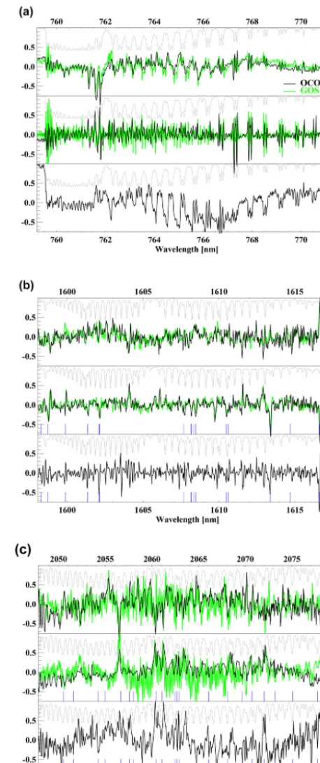
when the largest three EOFs were employed. The first two EOFs for GOSAT, as well as the first three EOFs for OCO-2, are shown in Fig. 7 for each spectral band. The EOFs for each of the eight spatial footprints sampled by OCO-2 are ex-tremely similar, though they are solved for independently due to the slightly different spectroscopic response of each. The first EOFs for OCO-2 and GOSAT are very similar for each band, indicating that common forward model errors such as spectroscopy and top-of-atmosphere solar flux, rather than instrument-specific effects, are driving the EOF patterns. The first EOF is also very similar to the mean residual pattern, and typically accounts for 50 %–60 % of the variance in the resid-uals. The second and third EOFs typically account for only 1 %–3 % of the variance in the residuals, with higher-order EOFs accounting for even less. For the O2A band, the
sec-ond EOF appears as a Doppler shift of the first. In the weak CO2band, the second EOF appears to be due to water vapor
lines, while the third EOF appears to be a Doppler shift of the first. Higher-order EOFs often exhibit additional instru-ment artifacts (such as unidentified bad spectral samples) and forward model errors related to water vapor, as well as other effects that are difficult to interpret.
The EOF formulation was modified in B8 in several ways. First, the EOFs were defined in terms of radiance per unit noise rather than pure radiance, in order to be consistent with the cost function metric that is minimized during the retrieval itself. However, the structure of the EOFs in B8 was much the same as in B7. Second, improved filtering of spectral samples that are contaminated by noisy or dead detector pixels greatly reduced their impact on the EOF patterns. Finally, a manual re-ordering of the EOFs was performed for each of OCO-2’s eight spatial footprints, because the standard ranking by variance would occasionally flip the EOF patterns in different footprints. This mattered because sometimes the third and fourth EOFs would change places (and the current algorithm only fits the first three EOFs). This ensured that, to the extent that the EOFs of each footprint roughly matched, the same three EOF patterns for each footprint are fit within the L2FP retrieval.
3.4 Surface model
The forward model for ACOS L2FP retrievals uses one of two surface models, depending on the location of the foot-print. Water surfaces are simulated as a linear combination of a Cox–Munk ocean surface (Cox and Munk, 1954) and Lam-bertian reflector. This surface has seven parameters: wind speed, and a Lambertian albedo at a reference wavenumber with a linear spectral slope term in each of the three spectral bands. The prior wind speed is taken from the resampled me-teorology (either ECMWF or GEOS5 FP-IT, as discussed in the next section), as for the other meteorological parameters. The strong CO2band Lambertian albedo is fixed to 0.02; the
other six terms are fit in an essentially unconstrained fashion. This approach leads to the fitted Lambertian albedos
gener-Figure 7.Spectral patterns of the EOFs for the O2A band(a), weak CO2 band (b), and strong CO2 band (c), for both GOSAT B3.5
(green) and OCO-2 B7 footprint 4 (black). For reference, the light gray trace in each panel shows the modeled spectrum (not to scale). Some stronger water vapor absorption lines (blue vertical lines) in the weak and strong CO2bands correlate with features in the second
ally staying small and positive, the latter of which is currently required by our radiative transfer module.
Through ACOS B7, land surfaces were assumed to be purely Lambertian, with an albedo and albedo spectral slope retrieved for each band. The Lambertian surface assumes that the bidirectional reflectance distribution function (BRDF; the ratio of the radiance in the reflected direction to the irradiance from the incident direction; Schaepman-Strub et al., 2006) is a constant that is often specified as a scalar albedo. Since in-dependent fits are done within each of the three OCO-2 spec-tral bands, this yields six state variables for land footprints.
Analysis of B7 OCO-2 target-mode observations showed that the retrieved Lambertian albedo and aerosol optical depth sometimes exhibited dependence on the sensor zenith angle for observations of the same surface location. This indicated that the true surface BRDF has dependence on the observation angles. A more physically justified approach would use a non-Lambertian model for the surface BRDF. For trace gas retrievals, a Lambertian surface assumption in-troduces no errors in the absence of multiple scattering be-tween the surface and atmosphere; in this case, the retrieved albedo is interpreted as the surface reflectance at the primary scattering geometry (Sun–surface–satellite). However, over brighter surfaces with some atmospheric scattering, the as-sumed BRDF could in principle affect the retrieval via the interaction of the retrieved aerosol, surface pressure, and gas concentrations. Therefore, in B8 it was decided to change the surface model for land footprints to a non-Lambertian surface model. This model assumes a fixed BRDF shape and assumes the surface is azimuthally symmetric, but al-lows for spectral dependence of the amplitude between and within each of our three bands; full details of the BRDF model are given in Appendix B. While this model does often show reduced correlation between view zenith and the re-trieved BRDF amplitude, the rere-trieved XCO2(as well as most other state vector parameters) shows very little change versus a version of the B8 retrieval run with a Lambertian surface. Therefore, while B8 does use a non-Lambertian BRDF pa-rameterization, a Lambertian surface appears to work equally well. This fact may be a consequence of the strong filtering used in B8, which tends to remove soundings with multiple scattering. Future applications of the ACOS L2FP algorithm to cases with higher AOD may be more strongly impacted by the non-Lambertian BRDF.
3.5 Additional retrieval algorithm changes
In addition to these changes, a number of additional (mostly minor) changes have also been made to the ACOS L2FP algorithm since B2.9. In B2.10, the prior CO2 profile was
changed to match that used by TCCON, which was more realistic than our previous prior formulation; as of B8, this corresponds to the GGG2014 version (Toon and Wunch, 2014). Generally speaking the TCCON CO2 prior profile
is relatively simple: it is a function of latitude, altitude,
Table 5.Median±1σ of GEOS5 FP-IT–ECMWF differences for GOSAT soundings passing the ABP cloud filter.
Variable Land Ocean
Surface pressure (hPa) 0.07±0.73 0.05±0.43 T2m (K) 0.4±2.7 0.3±0.6 T@700 hPa (K) 0.0±0.8 −0.2±0.8 TCWV (kg m−2) 0.1±1.8 0.4±2.4 Surface wind speed (m s−1) 0.4±1.3 −0.4±0.9
and date only. It includes a simple formulation of the sea-sonal cycle and currently assumes a fixed secular increase of 0.52 % yr−1(or 2.08 ppm yr−1at 400 ppm). There is no land– ocean or other meridional dependence. It requires specifying the tropopause height, and has simple formulations for the profile in the boundary layer, free troposphere, and strato-sphere. A small mistake in the XCO2 averaging kernel was also fixed in B2.10; this was caused by inconsistent assump-tions regarding the pressure-dependent gas absorption cross sections throughout our retrieval code, which led to an obvi-ous “kink” in the averaging kernel that had long been visu-ally evident (see, e.g., Fig. 2 of Connor et al., 2008). We use the 2016 version of the Toon solar transmittance spectrum (available at https://mark4sun.jpl.nasa.gov/toon/solar/solar_ spectrum.html, last access: 4 December 2018) (Toon, 2014). Changes in the prior covariance matrix for CO2 (O’Dell
et al., 2012) were also considered, but rejected, as tests us-ing alternate covariance matrices showed insignificant per-formance improvements.
In B3.3, solar-induced chlorophyll fluorescence (SIF) fit-ting over land surfaces was introduced. This change was in-troduced to combat a bias in XCO2 that results from not fit-ting for fluorescence when it is present, due to its impact on the O2A band. This problem and our fluorescence fitting
In B8, the prior height of the cirrus cloud layer relative to the surface pressure was moved slightly, from the fixed value of x=0.3 to just below the tropopause height (which is a relatively strong function of latitude). The calculation of the tropopause height itself was also refined in B8, which also improved the calculation of the prior CO2 profile. Finally,
the prior meteorology was changed in B8 from ECMWF to GEOS5-FP-IT (Suarez et al., 2008; Lucchesi, 2013). Some statistics regarding differences in surface pressure, tempera-ture, water vapor, and surface wind speed between the two models for retrieved GOSAT soundings are given in Table 5; the corresponding difference statistics for OCO-2 soundings are nearly identical. Only soundings passing the O2A band
prescreener are included. In general, the two models are very similar, with for instance 95 % of all soundings having a sur-face pressure difference of less than 1.5 hPa. Sursur-face pres-sure probably affects our retrieved XCO2 the most, as it is used not only in the retrieval, but also in the bias correction, where differences in the prior surface pressure will lead to a first-order change in the bias-corrected XCO2. Currently then, the “noise” from the surface pressure difference be-tween these two models would amount to roughly 0.6 hPa, or about 0.25 ppm in XCO2, which is quite a bit less than our noise-driven error (∼1.4 hPa on average) and regional biases (∼2.4 hPa on average). Retrieved surface pressure errors are discussed in more detail in Sect. 4.3.4.
4 Retrieval filtering and bias correction
All soundings passing the prescreening criteria (Table 1) are processed with the L2FP retrieval algorithm. Of these, some 10 %–20 % fail to converge to a solution, typically because of unscreened clouds or other factors that cannot properly be modeled in the retrieval. Some fail simply because of the nonlinear nature of the problem – in general, there is no per-fect way to minimize the cost function. Of the 80 %–90 % of soundings that do converge to a minimum in the cost func-tion, typically three to six iterations are required.
Despite our best efforts to prefilter problematic soundings, there are inevitably some retrievals with XCO2 errors that exceed those predicted by theory. Ideally, the XCO2 errors would be normally distributed, with errors consistent with the 1σ a posteriori uncertainty on XCO2 from the retrieval (see, e.g., Rodgers, 2000), but often there are retrievals with systematically biased XCO2and/or larger-than-expected scat-ter. This problem is partially mitigated by applying a bias correction, which can reduce both scatter on smaller spatial scales and biases on larger spatial scales. However, prob-lematic soundings still remain. A quality-filtering procedure then attempts to remove these soundings with larger-than-expected differences from our truth metrics. For GOSAT, this process was described in O’Dell et al. (2012) and Crisp et al. (2012). The problem of biases is dealt with via a linear bias correction (Wunch et al., 2011a). In this section, we describe
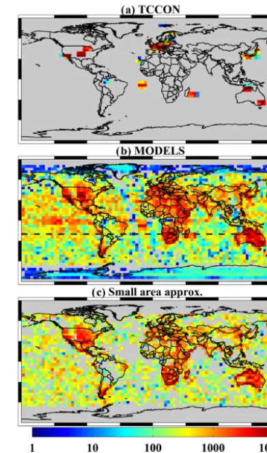
Figure 8.Sounding density of the truth proxy data in 4◦×4◦bins used in the OCO-2 version 8 XCO2 filtering and bias correction. (b) shows both the full global model-based truth proxy and the Southern Hemisphere truth proxy as the portion below the dashed black line.
both filtering and bias-correction procedures for XCO2for B8 retrievals only, unless otherwise noted. A similar procedure was used for GOSAT data as well as OCO-2 B7, but the pro-cedures were more mature and robust for B8.
4.1 Truth proxy training data sets
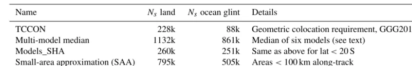
Table 6.XCO2 truth proxies for retrieval evaluation.
Name Ns land Nsocean glint Details
TCCON 228k 88k Geometric colocation requirement, GGG2014
Multi-model median 1132k 861k Median of six models (see text) Models_SHA 260k 251k Same as above for lat<20 S Small-area approximation (SAA) 795k 505k Areas<100 km along-track
4.1.1 TCCON-based truth proxy
The most direct truth proxy is the comparison to TCCON, which currently has 25 operational stations globally, but with heavy representation in North America, Europe, Asia, and Oceania. For the OCO-2 B8 evaluation, the latest version of TCCON retrievals was employed (GGG2014, Wunch et al., 2015). Many schemes have been used to match air masses observed by satellites to those viewed from TCCON stations. Examples include a geographic-centric scheme (Cogan et al., 2012; Inoue et al., 2013; Oshchepkov et al., 2013; Kulawik et al., 2016), a scheme based on the potential temperature at 700 hPa (Keppel-Aleks et al., 2011; Wunch et al., 2011b), model-based selection (Guerlet et al., 2013), and geostatisti-cal selection (Nguyen et al., 2014). These more sophisticated techniques were primarily used because GOSAT had fairly sparse data and required relatively loose matching criteria to yield sufficient numbers of matched observations. This is less of a problem with OCO-2 at lower and mid latitudes, with its higher spatial sampling density. High-latitude validation with TCCON remains challenging, where OCO-2 data are still sparse.
Table 7 lists the TCCON sites used as truth proxies in this work. Training data ranges correspond to the quality-filtering and bias-correction procedures described in Sect. 4.2 and 4.3, respectively. Validation data ranges correspond to the basic validation described in Sect. 5. Our colocation requirements for B8 were similar to those used for Wunch et al. (2017), in which we required that OCO-2 footprints were within 2.5◦ latitude and 5.0◦ longitude of the TCCON station, and that the observations occurred within 2 h of each other. These requirements were modified slightly for the Caltech, Arm-strong, and Tsukuba stations in order to discriminate satellite observations taken over the nearby megacities of Los An-geles and Tokyo. Because of additional station data and a longer training period, there were roughly twice as many sta-tion months of valid colocasta-tions for B8 as compared to our B7 training (roughly 400 versus 190 station months).
We estimate TCCON colocation errors to be on the or-der of 0.5 ppm, due to both colocation errors and TCCON station-level biases (Hedelius et al., 2017). Even with these small errors, TCCON is an incomplete validation source due to its limited spatial coverage. For example, there are few sta-tions in the tropics, none in the central Pacific or central Asia, and, with the exception of Armstrong, none in bright desert
regions. Except when specifically stated, we employed the OCO-2 averaging kernel correction. A general treatment of averaging kernel corrections was first given in Wunch et al. (2011a). The specific correction we employ is taken from Nguyen et al. (2014), in which the TCCON-retrieved profile is convolved with the OCO-2 column averaging kernel be-fore it is compared to OCO-2. This effect is generally smaller than 0.3 ppm in the column.
4.1.2 Small-area approximation truth proxy
To supplement TCCON, we used a method new for OCO-2 called the “small area approximation”, or SAA2. The SAA relies on the high spatial resolution of OCO-2 footprints (1.3×2.3 km2), and the relatively long decorrelation length of CO2concentration in the atmosphere (500–1000 km; see,
e.g., Chevallier et al., 2017, Fig. 1). Specifically, this approxi-mation assumes that for a given overpass of an area not larger than 100 km in spatial extent, XCO2 can be considered uni-form over the area. True XCO2 variability was evaluated by Worden et al. (2017) by examining output from the GEOS-5 7×7 km2“nature run”. It was found to be typically less than 0.1 ppm per 100 km areas away from strong known sources, thus justifying our small area assumption. In fact, this error is considerably lower than can be obtained by any of the other truth metrics. The major drawback of this method is that it is insensitive to biases due to variables that vary slowly on these small scales, such as those related to viewing geometry and some surface and aerosol parameters.
4.1.3 Model-based truth proxies
The third validation data set is based on results from global carbon flux inverse models, and is referred to as the “multi-model median”. In order to evaluate OCO-2 retrievals against a posteriori results from an array of models, and to avoid the biases in one particular model, a suite of six models sampled at the OCO-2 sounding locations and times was used. Table 8 provides a summary of the models that were used. The mod-els generally differed in their prior flux assumptions, prior flux uncertainty, transport model, initial conditions, spatial resolution, and inverse method, but had one commonality in that all assimilated in situ CO2 concentration data.
Be-cause of these differences, the models often yielded a
Table 7.TCCON stations used in this work.
TCCON station Training date range Validation date range Reference
Anmyeondo, South Korea May 2015–Sep 2015 May 2015–Aug 2016 Goo et al. (2014) Ascension Island Sep 2014–Dec 2016 Dec 2014–Feb 2017 Feist et al. (2014) Bialystok, Poland Sep 2014–Jun 2016 Sep 2014–Apr 2017 Deutscher et al. (2015) Burgos, Philippines Jan 2017 Mar 2017–Apr 2017 Velazco et al. (2017) Bremen, Germany Sep 2014–Jul 2016 Sep 2014–Mar 2017 Notholt et al. (2014) Caltech, Pasadena, CA, USA Sep 2014–Nov 2016 Sep 2014–Feb 2017 Wennberg et al. (2015) Darwin, Australia Sep 2014–Sep 2016 Sep 2014–Oct 2016 Griffith et al. (2014a) Edwards (Armstrong), CA, USA Sep 2014–Jun 2016 Sep 2014–Aug 2016 Iraci et al. (2016) East Trout Lake, Canada Jan 2017 Oct 2016–May 2017 Wunch et al. (2016)
Eureka, Canada Jun 2015 Aug 2015 Strong et al. (2016)
Garmisch, Germany Sep 2014–Aug 2016 Sep 2014–May 2017 Sussmann and Rettinger (2014) Izaña, Tenerife, Spain Dec 2015–Mar 2016 Dec 2015–Jul 2016 Blumenstock et al. (2014) Karlsruhe, Germany Sep 2014–Jun 2016 Sep 2014–May 2017 Hase et al. (2015) Lamont, OK, USA Sep 2014–Feb 2017 Sep 2014–May 2017 Wennberg et al. (2016) Lauder, New Zealand Sep 2014–Mar 2017 Sep 2014–May 2017 Sherlock et al. (2014) Manaus, Brazil April 2015–May 2015 Nov 2014–Jun 2015 Dubey et al. (2014) Ny Ålesund, Spitzbergen, Norway Not used May 2015–May 2017 Notholt et al. (2017) Orléans, France Sep 2014–Oct 2016 Sep 2014–May 2017 Warneke et al. (2014) Paris, France Apr 2015–Mar 2016 Oct 2014–Oct 2016 Te et al. (2014) Park Falls, WI, USA Sep 2014–Dec 2016 Sep 2014–May 2017 Wennberg et al. (2014) Réunion Island Sep 2014–Nov 2016 Sep 2014–May 2017 De Mazière et al. (2014) Rikubetsu, Japan Oct 2014–Oct 2016 Oct 2014–Feb 2017 Morino et al. (2016b) Saga, Japan Sep 2014–Mar 2016 Sep 2014–May 2017 Kawakami et al. (2014) Sodankylä, Finland Oct 2014–Jul 2016 May 2015–May 2017 Kivi and Heikkinen (2016) Tsukuba, Japan Sep 2014–Feb 2017 Sep 2014–May 2017 Morino et al. (2016a) Wollongong, Australia Sep 2014–Nov 2016 Sep 2014–May 2017 Griffith et al. (2014b)
Table 8.Models used in this work.
Name Version Land biosphere Inverse method Transport Reference
CAMS 15r2 ORCHIDEE 4D-Var LMDZ Chevallier et al. (2010) Univ. Edinburgh v2.1 CASA EnKF GEOS-Chem Feng et al. (2009) Jena CarboScope s04_v3.8 Special 4D-Var TM3 Rödenbeck (2005)
CarbonTracker CT2015, CASA EnKF TM5 Peters et al. (2007), with updates
CT-NRT.v2016-1 documented at https://carbontracker.noaa.gov (last access: 4 December 2018)
TM5-4DVar 2016 CASA 4D-Var TM5 Basu et al. (2013) OU 2016 CASA 4D-Var TM5 Crowell et al. (2018b)
riori XCO2 fields that disagreed to some extent, with differ-ences ranging from a few tenths of a ppm to several ppm as discussed below. We used model output that covered a minimum period from September 2014 through December 2015, though a few models (CarbonTracker, TM5-4DVar) extended into March 2016. To compare against the models, for simplicity we computed only true XCO2values from the a posteriori CO2concentrations, rather than
averaging-kernel-corrected values. Previous authors have shown that this ef-fect is typically small, on the order of a few tenths of a ppm (Wunch et al., 2011a; Inoue et al., 2013; Lindqvist et al., 2015).
Figure 9.Maximum difference between each model and the model median in ppm, averaged over 4◦×4◦grid boxes. Two seasons are shown: DJF(a)and JJA(b). Soundings for which all models are within 1.5 ppm of the model median are retained in the model-based truth proxy.
Figure 9 shows maximum difference from the model me-dian for both the Northern Hemisphere winter (December, January, February; DJF) and summer (June, July, August; JJA). Most soundings passed our “model-agreement” re-quirement over ocean at all times and over land in DJF, where the bulk of the land biosphere is quiet and hence XCO2 is more robustly modeled. In JJA, however, a substantial frac-tion of land soundings fail this test, in particular over North-ern Hemisphere regions such as Asia. Tests showed that our results were not strongly sensitive to the agreement threshold chosen.
Finally, Wunch et al. (2011a) used a truth proxy called the “Southern Hemisphere Approximation” (SHA) in which it was assumed that the Southern Hemisphere (25–55◦S) could be taken to be meridionally uniform in XCO2 at any given time, with a latitudinal gradient of−1 ppm from 25 to 55◦S, and the change in mean XCO2 over time could be pre-scribed with a linear secular trend (taken to be 1.9 ppm yr−1). This served reasonably well for the GOSAT retrievals at that time, which exhibited rather large errors. However, the SHA has the primary shortcoming that meridional anomalies can sometimes exceed 0.5–1.0 ppm and are typically larger over land versus ocean. We find that substituting the model me-dian instead of the zonally corrected mean used in Wunch et al. (2011a) results in error variances of the approxima-tion 3–4 times lower, when comparing against any particular model as truth. Therefore, in order to maintain a connection to the truth metric of Wunch et al. (2011a), in this work we adopt the modified SHA called “Model_SHA”. This is sim-ply the model median, discussed above but only used in the Southern Hemisphere below a latitude of 20◦S.
4.2 Quality filtering
The construction of the operational OCO-2 filtering and bias correction for B7 is described in detail in Mandrake et al. (2015), with updates for B8 described in an online user’s guide (Eldering et al., 2017b). The training procedure for both filtering and bias correction for these two versions
fol-lowed a similar approach. Below, we discuss the filtering and bias correction for version 8 only, and make notes where ver-sion 7 differed significantly. The filtering procedure yields two quantities. The first is a binary flag denoted the XCO2 quality flag, which requires that a series of parameter-based tests are all passed. The second is a graded set of “warn levels”, which assigns each retrieval an integer value from 0 (most likely to yield accurate XCO2) to 5 (least likely to yield accurate XCO2). A genetic algorithm (Mandrake et al., 2013) finds combinations of variables that are best at pre-dicting variance reduction in XCO2 over both small areas (.10×80 km2) and in the Southern Hemisphere (south of 25◦S). In this document, we focus only on the quality flag filtering.
Filtering is accomplished by first identifying variables that cause the largest δXCO2, where δXCO2 is defined as the retrieved–true XCO2, the latter of which is evaluated for a given truth proxy. This was done sequentially, by identify-ing the sidentify-ingle variable responsible for the largest fraction of the variance inδXCO2. We then created a simple threshold-based filter for this variable. After application of the filter, this process was repeated multiple times until it appeared that the majority of problematic data were removed. Because bias correction affected this procedure, a preliminary filter set was first created, after which a preliminary bias correction was developed. The preliminary bias correction was then ap-plied,δXCO2 was updated accordingly, and the filters were re-derived using this bias-corrected δXCO2. Generally this had only a minor effect on the filters, and often served to increase the fraction of data passed through filtering.
Figure 11.Same as Fig. 10 but for ocean glint measurements, where the truth proxy is the multi-model median.
ing variables selected and their thresholds were the same or similar, regardless of the particular truth proxy used.
An example of this sequential filtering approach is shown in Fig. 10, which shows the XCO2 error versus filtering pa-rameters for nadir and glint land soundings, using TCCON as the truth proxy. Overall, the results were found to be ro-bust for all our truth proxies. Just a few variables do the bulk of the filtering. For both land and ocean, the CO2and H2O
ratios computed by the IMAP-DOAS preprocessor account for a significant fraction of the total filtering. These variables represent the ratio of the total column CO2(H2O) as derived
from the weak CO2band to that from the strong CO2band.
As discussed at length in Taylor et al. (2016), values of these gas ratios that deviate significantly from unity indicate the presence of significant atmospheric scattering. As shown in Fig. 10, ratios significantly away from the median values can result in both large scatter and large biases. Another robust finding is that biases are associated with large absolute val-ues of the retrieved–prior surface pressure (dP) for both the Level-2 and ABP preprocessor retrievals. All of these vari-ables (CO2 and H2O ratios and surface pressure) are most
likely diagnosing scattering-induced errors due to improp-erly modeled clouds and aerosols.
Two variables associated with small-scale variability are also associated with increased scatter: the standard deviation of the surface altitude within OCO-2’s field-of-view, and an-other parameter called “Max_Declocking”, which is deter-mined independently for each of the three OCO-2 bands. The latter is related to a slope in the observed radiance within an individual sounding’s field-of-view, and is determined from OCO-2’s color slices as discussed in Crisp et al. (2017). The scatter associated with surface elevation appears to be re-lated to an instrument-to-spacecraft offset specification error, which results in small (several hundred meters) pointing er-rors, which is improved in the next data version (version 9) and allows for relaxation of this filter (Kiel et al., 2018).
Another interesting variable that can result in both bias and scatter is the tropospheric lapse rate of the retrieved CO2
pro-file, called co2_grad_del. It is determined by the difference in retrieved CO2between the surface and the retrieval
quantity for the prior:
co2_grad_del=[c(1)−c(0.7)]−cap(1)−cap(0.7), (5)
wherec(x)andcap(x)respectively denote the retrieved and
a priori CO2 dry air mole fraction at relative pressure x.
The reason why this variable is strongly associated with bias and scatter is still being investigated; it may be due to CO2
spectroscopy errors, or some other factor. There is also a fil-ter associated with dark surfaces; scenes with a strong CO2
band albedo less than 0.05 consistently exhibit a bias in re-trieved XCO2and are thus excluded. Note this will tend to flag most snow- and ice-covered surfaces (such as over Green-land and Antarctica), which are highly absorbing at wave-lengths longer than about 2 µm. It also tends to exclude dark forests such as in the Amazon. There are also filters associ-ated with the retrieved slope of the strong CO2band albedo,
the fit quality in the CO2 bands, and a number of retrieved
aerosol variables. Of particular note is the total retrieved opti-cal depth associated with our larger aerosol types: dust, water cloud, and sea salt (DWS). High values of DWS are associ-ated with negative biases in XCO2 over land, and it is used as both a filter and bias-correction variable. Although ice is also a large type, it is confined to the upper atmosphere in our retrieval and has its own dedicated filter.
Similar variables are used for filtering over water surfaces (Fig. 11), though note that almost no aerosol-related vari-ables are used. This may be because water surfaces have relatively uniform optical properties, such that the retrieved variables indirectly associated with cloud and aerosol scat-tering, such as the CO2and H2O ratios and the slope of the
strong CO2 band albedo, are more effective than over land,
obviating the need for additional aerosol-related filtering. It may also be because most downward-propagating, forward scattered light is absorbed by the ocean surface, so the path-ways for aerosol contamination are significantly less than over land, as noted by Butz et al. (2013).
As seen in the upper left panel of Fig. 11, the dominant filtering variable for water-glint soundings is the slope of the strong CO2 band albedo. This is the slope of the
re-trieved Lambertian albedo in that band, which is generally small and is added onto the reflectivity coming from the pri-mary Cox and Munk surface, which is a function of wind speed only. Negative slopes are strongly associated with XCO2 bias, which appears indicative of either cloud ice or sea salt aerosol scattering, both of which yield a negative slope in these units3. Large positive values of this slope are likely associated with contamination by sulfate aerosol or other small particle types. The sensitivity of this variable to cloud and aerosol scattering has been confirmed with simu-lations. About 10 % of water-glint soundings are flagged by this filter.
3The units of the albedo slope are in per unit wavenumber,
in-creasing with wavenumber.
After filtration, about 31 % of land soundings and 55 % of water soundings pass the XCO2 quality flag
4. As depicted in
Fig. 12, the pass rates are not uniformly distributed around the globe. Over land, very bright and dark surfaces are pref-erentially filtered out, as well as locations with many low clouds such as the Amazon, which are sometimes missed by our prefilters (Taylor et al., 2016). Nearly all soundings over ice surfaces are filtered out, because the albedo of ice is very low at 2 µm, hence yielding low signal-to-noise. The higher quality of water soundings is likely due to higher uniformity of water surfaces in glint mode, higher and more uniform SNR in all three bands, and fewer surface–atmosphere scat-tering mechanisms. Over both land and water, soundings at higher solar zenith angles are also removed at a higher rate by our quality flag. This is most likely due to the relatively large effects of scattering on our retrievals for these geome-tries, specifically when the fraction of the light received at the detector from atmospheric scattering is a larger fraction of the total. Over water, approximately 70 % of soundings pass at lower viewing angles, while nearly all soundings fail at high viewing angles.
4.3 Bias correction
After filtering, systematic biases remain in retrieved XCO2 which must be corrected in order to minimize errors. The OCO-2 bias correction contains three main pieces: para-metric, footprint-level, and global biases. Parametric bi-ases are functionally related to a given parameter associ-ated with a given sounding. Examples of this could be sur-face pressure, albedo quantities, or retrieved aerosol quanti-ties. Footprint-level biases are corrected to ensure that each of OCO-2’s eight sensors, or “footprints”, yield the same XCO2 value when observing similar scenes. This is not al-ways the case due to small calibration errors in the eight in-dividual footprints. The final step of the bias correction re-moves any global mean bias that may remain. The overall bias-correction equation is then written as
XCO2,bc=
XCO2,raw−CP(mode)−CF(j ) C0(mode)
, (6)
whereCP is the mode-dependent parametric bias,CF is the
footprint-dependent bias for footprintsj =1. . .8, andC0
rep-resents a mode-dependent global scaling factor. The follow-ing subsections discuss each of these corrections in detail. 4.3.1 Bias correction: parametric biases
The most complex but most important of the three aspects of the bias correction is inferring biases dependent upon
differ-4Note that these passing rates are lower than those in Figs. 10