University of Pennsylvania
ScholarlyCommons
Publicly Accessible Penn Dissertations
1-1-2015
Bank Regulations, Fiscal Policies and Growth
Thien Tung Nguyen
University of Pennsylvania, thien.tung.nguyen@gmail.com
Follow this and additional works at:
http://repository.upenn.edu/edissertations
Part of the
Economics Commons
, and the
Finance and Financial Management Commons
This paper is posted at ScholarlyCommons.http://repository.upenn.edu/edissertations/1104
For more information, please contactlibraryrepository@pobox.upenn.edu.
Recommended Citation
Nguyen, Thien Tung, "Bank Regulations, Fiscal Policies and Growth" (2015).Publicly Accessible Penn Dissertations. 1104.
Bank Regulations, Fiscal Policies and Growth
Abstract
This dissertation studies the effects of economic policies on investment, growth and welfare. The first chapter examines the welfare implications of bank capital requirements in a general equilibrium model in which a dynamic banking sector endogenously determines aggregate growth. Due to government bailouts, banks engage in risk-shifting, thereby depressing investment efficiency; furthermore, they over-lever, causing fragility in the financial sector. Capital regulation can address these distortions and has a first-order effect on both growth and welfare. In the model, the optimal level of minimum Tier 1 capital requirement is 8%, greater than that prescribed by both Basel II and III. Increasing bank capital requirements can produce welfare gains greater than 1% of lifetime consumption.
The second chapter studies fiscal policy design in an economy in which endogenous growth risk and asset prices are a first-order concern. When (i) the representative household has recursive preferences, and (ii) growth is endogenously sustained through R&D investment, fiscal policy alters both the composition of intertemporal consumption risk and the incentives to innovate. Tax policies aimed at short-run stabilization may substantially increase long run tax and growth risks and reduce both average growth and welfare. In contrast, policies oriented toward asset price stabilization increase growth, wealth and welfare by lowering the slope of the term structure of equity yields.
Degree Type Dissertation
Degree Name
Doctor of Philosophy (PhD)
Graduate Group Finance
First Advisor Amir Yaron
Keywords
Bailout guarantee, Bank regulation, Basel II, Basel III, Capital requirements, Risk-shifting
Subject Categories
BANK REGULATIONS, FISCAL POLICIES AND GROWTH
Thien T. Nguyen
A DISSERTATION
in
Finance
For the Graduate Group in Managerial Science and Applied Economics Presented to the Faculties of the University of Pennsylvania
in
Partial Fulfillment of the Requirements for the
Degree of Doctor of Philosophy
2015
Supervisor of Dissertation
Amir Yaron
Robert Morris Professor of Banking & Finance, Professor of Finance
Graduate Group Chairperson
Eric Bradlow
K.P. Chao Professor, Marketing, Statistics, and Education
Dissertation Committee
Amir Yaron, Robert Morris Professor of Banking & Finance, Professor of Finance Mariano Massimiliano Croce, Associate Professor of Finance
Itay Goldstein, Joel S. Ehrenkranz Family Professor, Professor of Finance Joao F. Gomes, Howard Butcher III Professor of Finance
ABSTRACT
BANK REGULATIONS, FISCAL POLICIES AND GROWTH
Thien T. Nguyen
Amir Yaron
This dissertation studies the effects of economic policies on investment, growth and welfare.
The first chapter examines the welfare implications of bank capital requirements in a general
equilibrium model in which a dynamic banking sector endogenously determines aggregate
growth. Due to government bailouts, banks engage in risk-shifting, thereby depressing
investment efficiency; furthermore, they over-lever, causing fragility in the financial sector.
Capital regulation can address these distortions and has a first-order effect on both growth
and welfare. In the model, the optimal level of minimum Tier 1 capital requirement is 8%,
greater than that prescribed by both Basel II and III. Increasing bank capital requirements
can produce welfare gains greater than 1% of lifetime consumption.
The second chapter studies fiscal policy design in an economy in which endogenous growth
risk and asset prices are a first-order concern. When (i) the representative household has
recursive preferences, and (ii) growth is endogenously sustained through R&D investment,
fiscal policy alters both the composition of intertemporal consumption risk and the
incen-tives to innovate. Tax policies aimed at short-run stabilization may substantially increase
long run tax and growth risks and reduce both average growth and welfare. In contrast,
policies oriented toward asset price stabilization increase growth, wealth and welfare by
TABLE OF CONTENTS
ABSTRACT . . . ii
LIST OF TABLES . . . iv
LIST OF ILLUSTRATIONS . . . v
CHAPTER 1 : Bank Capital Requirements: A Quantitative Analysis . . . 1
1.1 Introduction. . . 2
1.2 Evidence on Bank Risk-Shifting . . . 9
1.3 Model . . . 10
1.4 Quantitative Assessment . . . 22
1.5 Conclusion . . . 30
CHAPTER 2 : Fiscal Policy and the Distribution of Consumption Risk . . . 40
2.1 Introduction. . . 41
2.2 Model . . . 46
2.3 Calibration . . . 61
2.4 Short-Term-Oriented Tax Smoothing and the Distribution of Risk . . . 63
2.5 Long-Term-Oriented Tax Smoothing . . . 77
2.6 R&D Subsidy and Expenditure Risks. . . 79
2.7 Conclusion . . . 82
APPENDIX. . . 85
LIST OF TABLES
TABLE 1 : Benchmark Calibration . . . 23
TABLE 2 : Main Statistics . . . 25
TABLE 3 : Calibration and Main Statistics . . . 62
LIST OF ILLUSTRATIONS
FIGURE 1 : Policy functions: risk-shifting. . . 31
FIGURE 2 : Policy functions: no risk-shifting . . . 32
FIGURE 3 : Welfare benefits . . . 33
FIGURE 4 : Consumption growth and distribution of banks. . . 34
FIGURE 5 : Welfare benefits, consumption and productivity . . . 35
FIGURE 6 : Role of probability of bailoutλ. . . 36
FIGURE 7 : Role of equity issuance costφ . . . 37
FIGURE 8 : Role of productivity loss due to risk-shiftingµ . . . 38
FIGURE 9 : Role of additional risk exposure due to risk-shiftingσ . . . 39
FIGURE 10 : Impulse Response of Tax Rate and Debt . . . 64
FIGURE 11 : Zero-deficit versus Strong Tax Smoothing: Impulse Responses in the CRRA Case . . . 66
FIGURE 12 : Zero-deficit versus Strong Tax Smoothing: Impulse Responses in the EZ Case . . . 67
FIGURE 13 : Welfare Costs and Patent Value in the CRRA Case . . . 70
FIGURE 14 : Welfare Costs and Patents’ Value in the EZ Case . . . 72
FIGURE 15 : Fiscal Policies and Term Structure of Profits . . . 74
FIGURE 16 : Utility Mean-Variance Frontier and the Role of IES . . . 76
FIGURE 17 : Welfare Benefits from Long-Run Stabilization . . . 78
FIGURE 18 : Welfare Costs with R&D Subsidy . . . 81
FIGURE 19 : Welfare Costs and Expenditure Risks . . . 83
CHAPTER 1 : Bank Capital Requirements: A Quantitative Analysis
Thien T. Nguyen
Abstract
This paper examines the welfare implications of bank capital requirements in a general
equilibrium model in which a dynamic banking sector endogenously determines aggregate
growth. Due to government bailouts, banks engage in risk-shifting, thereby depressing
investment efficiency; furthermore, they over-lever, causing fragility in the financial sector.
Capital regulation can address these distortions and has a first-order effect on both growth
and welfare. In the model, the optimal level of minimum Tier 1 capital requirement is 8%,
greater than that prescribed by both Basel II and III. Increasing bank capital requirements
1.1. Introduction
Following the recent financial crisis, a change to bank regulatory capital requirements has
become one of the key regulatory reforms under consideration as well as the subject of an
extensive academic debate (see Admati, DeMarzo, Hellwig, and Pfleiderer (2010)). There is a strong consensus among policymakers in favor of higher bank capital requirements.
The benefit of increased requirements is clear: having more capital helps banks better
absorb adverse shocks and thus reduces the probability of financial distress. More capital
would also reduce bank risk-taking incentives and thus improve investment efficiency and
overall welfare. The banking industry has adamantly pushed back the effort to increase
capital requirements however, arguing that an increase in the bank capital requirement
could adversely affect bank lending and leads to lower economic growth. For effective policy
making, it is thus vital to determine which effect dominates by quantitatively assessing the
welfare implications of higher bank capital requirements.
To contribute to the current debate, this paper analyzes the welfare implications of bank
equity capital requirements in a model with endogenous growth and a dynamic banking
sector. The endogenous growth framework is important because it allows bank regulation
to affect the growth rate of the economy. Banks play an important role in financing capital
production, which in turn is used to produce final goods. In the model, sustained growth
results from capital accumulation (Romer(1986)); therefore, any distortion in bank lending will have an effect on aggregate activities. This paper focuses on the distortions that
bank bailouts cause and the role that bank capital requirements play in mitigating these
distortions.1
To this end, banks in the model economy are taken to be big banks, which entails the
assumption that the government bails out banks with a high probability ex-post. This
1There are other motivations for regulating banks, for example, to prevent contagious effects of bank
can be motivated from the recent financial crisis: many large institutions were bailed out
through programs such as the Troubled Asset Relief Program (TARP) and the emergency
Federal Deposit Insurance Corporation (FDIC) Temporary Liquidity Guarantee Program.
This FDIC program guarantees bank debt and business checking accounts, which are not
normally covered under the FDIC’s deposit insurance. Nonetheless, the fall of Lehman
Brothers, Washington Mutual and Wachovia has shown that governments can and do permit
big banks to fail. The proposed model captures both dynamics.
The high probability of bailout implies that ex-ante bank depositors expect to be
com-pensated even if banks default, and hence banks do not have to remunerate depositors
entirely for bank default risk. Thus deposits are a cheap source of funding for banks. This
causes banks to over-lever. Moreover, given the option to default due to limited liability,
banks have incentives to risk-shift, lending to risky and less productive firms. This lending
practice allows banks to reap the benefits when they succeed but escape costs when they
fail. Risk-shifting by bankers has welfare implications because funds are used inefficiently.
In addition to prospective government bailouts, other factors that determine bank capital
structure in the model are bank default cost and equity issuance cost.
When calibrated to match key moments in the distribution of U.S. banks as well as
macroe-conomic quantities, the model produces a hump-shape in welfare, with the optimum at an
8% minimum Tier 1 capital requirement. This is 2 percentage points higher than the level
of Tier 1 capital ratio recommended by Basel III in 2010, a measure that was adopted by
U.S. regulators in July 2013, and 4 percentage points higher than the Basel II requirement.
Relative to the 4% Basel II minimum Tier 1 capital ratio, the 8% level improves welfare
by 1.1% of lifetime consumption. That is, requiring banks to hold a minimum of 8% in
equity capital is equivalent to giving the representative agent with a 4% minimum capital
requirement a 1.1% increase in consumption every period. What is more important is that
welfare gains remain sizable even at very high levels of capital requirement.
raise funds from depositors to exploit the subsidy implicit in government bailouts. Banks,
therefore, can provide more credit for capital production, which results in more capital
being produced, leading in turn to higher growth. However, at low levels of bank capital
requirements, because banks have the default option and do not have enough “skin in the
game,” they engage in risk-shifting, lending to risky-low-productivity firms. Consequently,
the average investment productivity in the economy is low and the rate of bank default is
elevated, which leads to high capital losses. Therefore, in order to attain high growth, since
investment is inefficient, substantial resources are used for capital production, and little is
left for consumption. The net effect is lower welfare despite higher growth.
As the minimum capital constraint increases, so does the shadow cost of funding for banks.
Moreover, the extent to which banks can exploit the implicit subsidy using deposits reduces,
and a larger proportion of banks have to issue equity, for which they have to pay issuance
cost. Therefore, more banks exit the economy, aggregate credit is tightened, less capital
is produced, and growth is lowered. At the same time, however, bank lower leverage and
lower incentive for risk-shifting result in lower default and higher overall capital production
productivity and consumption. The effect on increasing productivity and consumption
dom-inates the lowered growth and leads to a graduate increase in welfare, reaching a maximum
of 1.1% of lifetime consumption when the capital requirement is at 8%.
As the capital requirement increases above 8%, lower welfare gains result. The reasons are
twofold. The first is equity flotation costs. Since banks must pay issuance costs and these
are rebated back to households, the private cost of issuing equity is higher than the social
cost. Therefore, the funds that are raised are lower than those in a centralized economy.
This leads to lower lending, lower capital production, and hence lower growth. The second
reason is the presence of the “learning-by-doing” spillover that is inherent in the Romer
(1986) endogenous growth model. In this class of models, capital accumulation improves overall final good production productivity, and because this is external to each individual
accumulation. Consequently, any policy that further discourages investment lowers welfare.
In the current setup, higher bank capital requirements increase the private cost of capital
for banks, causing a reduction in lending and thus a lower accumulated stock of capital.
This brings the decentralized allocations further away from the first-best allocation and
lowers welfare gains.
To the best of my knowledge, the proposed model is the first, in a fully specified dynamic
general equilibrium setting, to quantitatively investigate the impact of capital requirements
on deterring moral hazard, on financing and hence growth.
1.1.1. Related Literature
This paper is at the intersection of a large literature on banking and macroeconomics. On
the macroeconomic side, this study is related to a burgeoning strand of literature started
byKung and Schmid(2011) that uses endogenous growth models to generate long-run con-sumption growth risk, a feature that is essential for explaining asset market data (Bansal and Yaron (2004b)). Croce, Nguyen, and Schmid (2012) examine the link between fiscal policies and pessimism in the spirit of Hansen and Sargent (2010). Croce, Nguyen, and Schmid (2013) analyze fiscal policy design when there is a tradeoff between short-run sta-bilization and long-run growth risk. More closely related to the setup in the present paper,
Opp(2010) focuses on the role of the financial sector in amplifying shocks in a Schumpete-rian growth model.
On the banking side, there are many theoretical studies on moral hazard due to public
guarantees. In the context of deposit insurance, Merton (1977) shows that deposit insur-ance provides banks with a put option, and thus without any regulation banks would find
it privately optimal to take on more risk. Furthermore,Mailath and Mester(1994) analyze bank closure policy and show that over a wide region of parameters, “too-big-to-fail” banks
arise in equilibrium and can lead to excessive risk-taking. There is also a strand of
charter value for banks because banks then benefit from the lower cost of funding. This
induces banks to be more conservative in lending, because they have more to lose in default
(Keeley (1990)). Cordella and Yeyati (2003) and Hakenes and Schnabel (2010) show that the net effect on risk-taking depends on which channel dominates. Consistent with these
theoretical predictions, in the present paper banks risk-shift only when their charter values
are sufficiently low, and they do not engage in risk-shifting otherwise.
The main instrument used by regulators to restrict bank risk-shifting incentive is minimum
capital requirements, and there are many theoretical studies on the effectiveness of this
instrument. For example, Hellmann, Murdock, and Stiglitz (2000), Repullo (2004), and
Morrison and White (2005) analyze the role of capital in disciplining bank moral hazard.
Allen, Carletti, and Marquez (2011) study capital regulation in the case in which credit market competition induces banks to hold capital in excess of the regulatory constraint, a
fact that is robust in the data. The authors show that the decentralized solution entails
banks’ holding a level of capital higher than the regulatory solution. In a similar vein,
Mehran and Thakor (2011) argue that there is a positive link between bank capital and bank value because bank capital encourages monitoring; the authors also provide empirical
support for their theoretical prediction. Acharya, Mehran, and Thakor(2012) study bank capital requirements when banks face asset substitution by shareholders and rent-seeking
by managers, and they analyze the trade-offs of the use of capital regulation to reduce
risk-taking vs. allowing debt to discipline managerial rent-seeking. Harris, Opp, and Opp
(2013) examine the effectiveness of bank capital requirements in the existence of competition between regulated banks and unregulated investors. They show that when competition is
sufficiently strong, bank capital regulation becomes ineffective. The extant literature thus
far has not focused on the impact of capital requirements on growth, however; the present
paper addresses this gap in the literature.
Empirical studies related to the impact of higher bank capital requirements on lending and
percentage point increase in the capital ratio, the long-run steady-state weighted average
cost of capital for banks increases by 25–45 basis points. Baker and Wurgler(2013) estimate the impact on average cost of capital of the same policy to be 60–90 basis points. In an
interesting study exploiting data on a costly loophole used to bypass the capital requirement,
Kisin and Manela(2013) show that a 10 percentage point increase in the capital ratio leads to at most a three basis points increase in banks’ cost of capital. These studies shed light
on the potential impact of capital requirements on real activities; however, it is difficult to
conclude whether such a policy would be beneficial due to the uncertain and potentially
nonlinear general equilibrium effects from a substantial increase in the capital ratio. My
paper complements these studies in this respect.
Quantitative studies on the welfare impact of bank capital requirements are even more
limited. Van den Heuvel (2008) was the first to quantitatively study the welfare cost of bank capital requirements. Using yield spread data, he shows that U.S. regulation at the
time was too high due to a reduction in liquidity creation. Corbae and D’Erasmo (2012) study capital requirements when there is competition between big and small banks. They
find that an increase in the capital requirement leads to a fall in the loan supply and a rise
in the interest rate. However, neither Van den Heuvel (2008) nor Corbae and D’Erasmo
(2012) address the concern on the effect of capital regulation on growth, which is at the heart of the current policy debate.
In this paper, banks optimally determine their capital structure by trading off bank default
costs, the benefit of implicit guarantees, and equity issuance costs, all while operating in an
endogenous growth environment. Thus, the present study complements the literature on
understanding the welfare implications of capital regulations. This paper is the first, to the
best of my knowledge, to quantitatively investigate the impact of capital requirements on
growth and risk-shifting in a fully specified dynamic general equilibrium banking model.
More broadly, my paper is related to the macro literature in which models contain financial
premia and asset volatility in crises in a setup in which financial intermediary capital plays
an important role in pricing assets. He and Krishnamurthy (2011) and Brunnermeier and Sannikov (2013) focus on the amplification of shocks, where in equilibrium the economy can enter systemic crisis states. Adrian and Boyarchenko (2012) study leverage cycles in a model in which financial intermediaries can produce capital more efficiently than
house-holds and intermediary leverage is restricted by a value-at-risk constraint. They show that
this constraint plays an important role in amplifying shocks; moreover, varying the
tight-ness of the value-at-risk constraint produces an inverted U-shape in households’ welfare.
As the authors pointed out, however, this result depends on the assumption that
inter-mediaries finance themselves only with debt. Moreover, as is common in this literature,
Adrian and Boyarchenko’s paper relies on heterogeneity in preferences between financial intermediaries and households. This makes it somewhat difficult to analyze welfare effects.
In my model, homogeneous households own all productive assets, and welfare is readily
comparable between different levels of capital constraint. Importantly, in my model
finan-cial intermediaries hold finanfinan-cial assets–giving loans to firms, instead of directly investing
in capital projects. This makes it easier to interpret these intermediaries as banks and
examine bank capital regulations.
In a different setup,Gertler and Kiyotaki(2013) examine bank instability in a model where households are subject to liquidity shocks, leading to bank runs as inDiamond and Dybvig
(1983). Gertler, Kiyotaki, and Queralto (2011) consider a model with financial interme-diation in which the intermediaries can issue outside equity as well as short term debt,
making intermediary risk exposure an endogenous choice. In a DSGE model with financial
The rest of the paper is organized as follows. Section 1.2 reviews evidence on bank
risk-shifting. Section 2.2 discusses the model, and Section 1.4 gives a quantitative assessment
of bank capital requirements. Section 1.5concludes.
1.2. Evidence on Bank Risk-Shifting
In the model described in this paper bailouts cause banks to risk-shift; this prediction is
well known within existing banking theories and has ample empirical support. As this is a
prominent feature of my model, I nonetheless review these evidence here. Gropp, Gruendl, and Guettler(2013) use a natural experiment in the removal of government guarantees for German savings banks; they show that after guarantees are removed, banks reduce credit
risk and adjust their liabilities away from risk-sensitive debt instruments. Moreover, their
bond yield spreads increase significantly. The authors conclude that public guarantees result
in substantial moral hazard effects. Furthermore, Dam and Koetter (2012) use a data set of actual bailouts of German banks from 1995–2006 and show that increases in bailout
expectations significantly heighten bank risk-taking.
In a recent study on risk-shifting,Duchin and Sosyura(2013) use data on bank applications for government assistance under the TARP and show that banks make riskier loans and shift
investment portfolios toward riskier securities after being approved for government
assis-tance. This is consistent with the moral hazard story, as an approved for assistance through
TARP signals government support going forward. In a related study,Black and Hazelwood
(2012) compare the risk ratings of commercial loan originations of TARP recipient and non-recipient banks and show that loan orginations risk increases at large TARP-recipient
banks. On a related note, Drechsler, Drechsel, Marques-Ibanez, and Schnabl (2013) use a unique data set from the European Central Bank (ECB) and show evidence that during
the recent financial crisis, of banks that borrow from the Lender of Last Resort–the ECB in
this case–those with lower financial strength borrowed more and pledged increasingly risky
collateral. The authors test four different theories and show that risk-shifting by banks is
There is also ample evidence of risk-shifting owing to another form of public guarantee:
deposit insurance. Grossman (1992) uses a data set of insured and uninsured thrifts in the 1930s and documents that after several years, insured thrifts engaged in relatively
riskier lending activities as measured by the foreclosures-to-assets ratio. Wheelock and Wilson (1995) show that deposit insurance membership increases the probability of bank failure. From cross-country evidence, using differences in the presence and design of deposit
insurance schemes,Demirguc-Kunt and Detragiache(2002) find that countries with explicit deposit insurance are more likely to have banking crises. All in all, existing empirical
evidence suggests that when there are public guarantees, banks engage in risk-shifting.
1.3. Model
The model consists of four types of agents: (1) households, who consume and save, (2)
final good producers, who produce the consumption good, (3) capital-producing firms,
who produce capital, and (4) banks, who raise funds from households and lend to
capital-producing firms. I will now describe each of the agents in turn.
1.3.1. Households
The economy is populated by a measure one of identical households who have CRRA
pref-erences over consumption Ct,
U0 =E0
∞ X t=0
βtC
1−1/ψ
t −1
1−1/ψ ,
whereψis the intertemporal elasticity of substitution andβ ∈(0,1)the subjective discount
factor. In every period, households are also endowed with one unit of labor, Lt = 1, and
since they do not value leisure, they supply labor inelastically. The discount factor can be
written as usual:
Mt+1 =β
Ct+1
Ct
−1/ψ
.
addition to equity shares, they hold deposits issued by banks. I assume that they can split
their deposits and equity shares equally among all banks, so that the law of large numbers
applies and all idiosyncratic risks, as will be specified in subsection 1.3.3 and 1.3.4 below,
are diversified away. All proceeds are returned to the household at the end of the period.
1.3.2. Final Good Production
There is a measure one of final good producers. Producer u∈[0,1]has technology
yut=Atkutα(Ktlut)1−α, (1.1)
whereAtis total factor of productivity,kut is produceru’s capital,lutis labor demand, and
Kt is the aggregate level of capital, which produceru takes as given. This is a simple way
to generate endogenous growth as in Romer(1986) via the “learning-by-doing” externality. Aggregate capital and labor are then simply
Z 1 0
kutdu=Kt (1.2)
and
Z 1 0
lutdu=Lt= 1. (1.3)
Since all producers function at the same capital-effective labor ratio, aggregate output can
be written as
Yt= Z 1
0
yutdu=AtKtLt1−α=AtKt. (1.4)
In aggregate, therefore, there is no diminishing return to capital despite diminishing return
at the individual final good producer level. This is the source of growth in the model.
Capital accumulation by an individual final good producer increases productivity by all
other producers through aggregate capital Kt, but since this is taken as external to the
producer, in the decentralized allocations there is under-investment. This externality on
Let pI
t be the relative price of capital. The final good producer u chooses investment idut and dividend dut to maximize shareholders’ value
v(ku,t−1, Kt, At) = max id
ut,dut,lut
dut+EtMt+1v(kut, Kt+1, At+1), (1.5)
subject to
dut =yut−Wtlut−pIt ·idut−
a
2
id ut
ku,t−1 2
ku,t−1 (1.6)
kut = (1−δ)ku,t−1+idut, (1.7)
whereδ is the depreciation rate of capital andWtthe equilibrium wage rate. The last term
in (1.6) captures investment adjustment costs, a standard assumption in the macrofinance
literature. Aggregate demand for the capital good is then
Itd=
Z 1 0
idutdu=idut,
where I am considering the symmetric equilibrium in which all final good producers behave
identically. The first-order condition with respect to capital implies that, in the symmetric
equilibrium, the price of capital satisfies the condition
pI
t =AtαL1t−α−a
Id t
Kt−1
+EtMt+1
pIt+1(1−δ) +
a
2
Id t+1
Kt !2
+a I
d t+1
Kt !
(1−δ)
. (1.8)
In equilibrium, aggregate capital demand must equal aggregate capital supply produced
by capital-producing firms. Since in the model financial frictions mainly affect the capital
supply, this is the channel through which bank regulations affect the whole economy.
1.3.3. Capital-Producing Firms
The economy consists of islands indexed byj.One can think of an island as an industry or a
to j that cannot be diversified away. On each island, at the beginning of each period, a
large number of infinitesimal capital-producing firms is born. These firms are short-lived.
Each firm is endowed with a project with a required investment of it today for production
tomorrow. itis taken as given by all agents in the economy. Those firms that get financing
invest today and then produce capital, settle payments, and exit the economy tomorrow.
Those that do not get financing exit the economy immediately. Then new firms are born.
Firms on any island are of two types: normal firms and risky-low-productivity firms. For
the normal firm, investingit today produceszj,t+1·it units of capital tomorrow, wherezjt
is an island-specific persistent shock:
logzj,t+1=ρzlogzjt+σzzj,t+1, ∀j.
As for the risky-low-productivity firm, investing it today produces zj,t+1jf,t+1·it units of
capital tomorrow, where jf,t+1 is specific to firm f in island j. This shock is independent
and identically distributed across firms, that is,
logjf t∼ N
−µ−1
2σ 2 , σ
∀j, f, t.
Therefore, risky-low-productivity firms are both riskier because they are exposed to an
additional shock, and on average less productive,µ≥0,than normal firms. The technology
for both type of firms can be written compactly as
zj,t+1·[χjf,t+1+ (1−χ)]·it,
whereχis an indicator function equal to one if the firm is a risky-low-productivity firm and
zero if it is a normal firm. To economize on notation, I drop the subscriptj where there is
no risk of confusion.
however can be raised within the households that own the firms, that is, for each firm, the
internal equity is enough to cover operating cost. As for the funds that must be invested
into the firms, it, because of unmodeled commitment or moral hazard frictions they
can-not borrow directly from other households. They can, however, approach banks for funds
because banks have a monitoring technology that solves the moral hazard problem.2 Since
there is a large number of firms on each island, firms behave competitively, and the lending
rateRlis determined by firms’ zero profit condition, taking into account the default option
and whether firm f is a risky firm:
EtMt+1max{0, pIt+1zt+1[χf,t+1+ (1−χ)]−Rl(χ, zt)}
| {z }
Firm’s default option
·it= o·it
|{z}
Operating cost
(1.9)
Recall thatpI
t is the market price of capital. Thus the left hand side of equation (1.9) is firm
f’s expected discounted revenue net of loan repayment. The ‘max’ operator captures the
fact that firm has the option to default on its loan if the proceeds from the sale of capital
are not enough to cover the loan repayment. The firm’s default option implies that there
exists a firm-specific cutoff in terms of the shock tomorrowz¯t+1(zt, χ, f,t+1)such that firm
f will default if the productivity zt+1 on the island falls below that level.
1.3.4. Banks
On each island, banks differ in the net cash, denoted by πt, that they have on hand at the
beginning of the period. If not exiting the economy, each bank must choose one firm to
2
finance.3,4 A bank’s revenues realized next period from lending this period are then
ˆ
πt+1(χt, zt, zt+1, f,t+1) =it
Rl(χt, zt)·1{zt+1≥z¯t+1} (1.10)
+η·pIt+1zt+1[χtf,t+1+ (1−χt)]
| {z }
Liquidated asset value
·1{zt+1<¯zt+1}
,
where η is the fraction of capital that could be recovered from the firm if it defaults, and
with a slight abuse of notation, where χt denotes the bank’s choice of the type of firm to
finance this period. This also means that there is no asymmetric information, and banks
know the type of firms to which they give loans.
If it finances a firm, a bank must spend resources to monitor it. In particular, I assume
the monitoring cost is m per unit of investment. One could think of this cost as the
intermediation cost of providing credit.
Each bank could finance its loan using a mixture of debt and equity. Letbt be the amount
of deposits outstanding andRb
t the required deposit rate. Further, let dt be the net equity issuance. The bank’s budget constraint is
ˆ
πt−Rbtbt | {z }
≡πt
−m·it+bt+1=it+dt, (1.11)
where the net cash,πt,is revenues from lending last period net of current deposit liabilities.
The left-hand side of (1.11) is the source of funding and the right hand-side is the use. In
addition to new debt bt+1 issued, the bank’s resources come from lending last period, net
of interest payments on deposits and monitoring costs. Funding is used for financing a firm
3One could think that each bank finances a portfolio of firms, which have a firm-level idiosyncratic shock.
By the law of large numbers, the firm-level idiosyncratic risk is diversified away, but because all firms are in the same island, the island-specific shock is not. Therefore, allowing banks to hold a portfolio of firms is equivalent to the current setup. Notice that when a bank wants to risk-shift, it wants exposure to a firm specific shock, and so it is optimal for a banknot to diversify this risk away.
4
this period and for paying dividends.
If the bank issues equity, i.e., dt < 0, it has to pay a flotation cost. To better match
quantity, as is common in the dynamic corporate literature, I assume that equity issuance
costs are proportional to the amount issued (Gomes (2001); Hennessy and Whited (2005,
2007);Gomes and Schmid(2010b)). In particular,
Φ(dt) =−φ·dt1{dt<0}. (1.12)
The indicator function means that this cost is only applied when the bank issues equity.
Distributions to bank shareholders are then just the equity payout net of issuance costs:
dt−Φ(dt). (1.13)
1.3.4.0.1 Bank equity valuation. Bank equity value is defined as the discounted sum
of all future distributions. If the prospect of operating is sufficiently bad, equity holders
will choose to close down the bank, i.e., the bank exits the economy. Conditional on the
bank exiting the economy, there are two distinct cases. The first is when lending revenue is
not enough to cover deposit liabilities. In this case, the bank will stop servicing its deposits
and exit; that is, the bank defaults. In the second case, the bank’s revenue is greater than
deposit liabilities, but economic prospects are sufficiently low that it is optimal for the bank
to close down and pay out its residual cash after servicing its depositors. The value of the
bank upon exit is then Vxt= max{0, πt}.The equity value of the bank is thus the solution
to the problem
Vt(zt, πt) = max{Vxt, max bt+1,χt,dt
subject to the loan demand schedule (1.9), the budget constraint (1.11), and the minimum
bank equity capital requirement
πt−m·it−dt
it ≥
¯
e, (1.15)
where the net cash next period is
πt+1 = ˆπt+1(χt, zt, zt+1, f,t+1)−Rbt+1bt+1. (1.16)
The denominator in (1.15) is the loan given to the firm, and that represents the bank’s
total assets. In the numerator, the first two terms are retained earnings and the last term is
the dividend payout (dt is positive) or the equity raised (dtnegative); thus, the numerator
represents the total equity that the bank uses to finance its assets. The minimum capital
requirement imposes that at least a fraction ¯eof the bank assets must be financed by the
bank equity capital.
1.3.4.0.2 Bank deposit valuation. When a bank decides to stop servicing its deposits,
depositors are bailed out with probabilityλ.To keep the analysis focus, bailouts are assumed
to be financed using a lump-sum tax, so that no additional distortion is introduced. If not
bailed out, depositors recover a fractionθ of the bank’s revenues.5 The market price of the
bank deposits satisfies the condition
bt+1=EtMt+1
Bank does not default
z }| {
Rbt+1bt+1·1{Vt+1>0} +
Bank defaults–bailed out
z }| {
λRbt+1bt+1·1{Vt+1=0}
+ (1−λ)θˆπt+1·1{Vt+1=0}
| {z }
Bank defaults–not bailed out
. (1.17)
5
Because of the probability of bailout, the bank does not have to compensate depositors fully
for the risk that it undertakes. Moreover since the bank has the option to default when its
loan goes bad, the bailout creates incentives for the bank to finance risky-low-productivity
firms. This is the typical risk-shifting that has been highlighted in the theoretical banking
literature discussed in sections1.1.1and 1.2.
1.3.4.0.3 Entry and exit. Every period, banks enter and exit the economy. As
dis-cussed earlier, banks exit when the prospect of operating is sufficiently low, that is, when
Vt=Vxt.
Each period a mass of potential new banks arrives in the economy. Entering entails a setup
cost that is proportional to asset size e·it. Since in this model growth is endogenous, all
quantities, including the equity value of the bank, grow at the same rate. The entry cost is
modeled proportional to investment to make sure it will not vanish in the long run relative
to trend and hence will stay relevant. The potential new bank observes the aggregate state
of the economy, but before knowing which island it will be on, it has to pay the setup
cost. Once the setup cost is paid, the potential new bank draws the initial shock from the
stationary distribution of zt.Thus, entry occurs if and only if
e·it≤EzVt(zt, πt= 0), (1.18)
where the expectation is taken with respect to the long-run distribution ofzt.The free-entry
condition (1.18) holds with equality when entry is positive.
1.3.4.0.4 Distribution of banks. The behavior of each bank is completely
character-ized by its individual state (zt, πt). We can thus summarize the aggregate distribution of
with state(zt, πt).The law of motion for the measure of banks is given by
Γt+1(zt+1, πt+1) =T((zt+1, πt+1)|(zt, πt)) [Γt(zt, πt) +Bt(zt, πt= 0) +Et(zt, πt= 0)].
(1.19)
Here Bt is the mass of banks that defaults and gets bailed out. They continue to operate
with zero net cash. Etis the measure of new banks, and they enter with no cash. Moreover,
for any setΘt+1 ⊂Z×Π, the space of possible combination of(z, π), T(Θt+1|(zt, πt))the
transition function is defined as
T(Θt+1|(zt, πt)) = Z
Z Z
Ω
1{(zt+1,πt+1)∈Θt+1|t+1}1{Vt>Vxt}dP(t+1)dQ(zt+1|zt), (1.20)
whereΩis the state space for ,the additional risk exposure for the risky-low-productivity
firm. The first indicator is one if given t+1,the pair(zt+1, πt+1)belongs toΘt+1,and zero
otherwise. The second indicator function takes into account the bank’s endogenous exit
decision. Q is the transition function for the exogenous shock z, and P is the cumulative
distribution function of theshock.
1.3.4.0.5 Bank capital structure and risk-shifting. In additional to the bank’s
charter value, which is endogenous in the model, bank capital structure is determined by
three forces: the equity issuance cost, the bailout probability, and the bank bankruptcy cost.
Fig. 1shows how risk-shifting is manifested in the model and how banks finance their loans
when they risk-shift. This figure plots the bank’s policy functions on a particular island,
where island-specific productivity is low. Because of low productivity, the bank’s charter
value is sufficiently low, and this leads all banks on the island to engage in risk-shifting
(top right panel). If they do not exit (when the exit decision is zero in the top left panel
of Fig. 1), they lever up as much as they can, reaching the minimum capital constraint
(bottom left panel), and pay out all their cash as dividends (bottom right panel). This is
intuitive. Because banks have the option to default, if they want to risk-shift, they do not
whereas if they fail they will lose the minimum amount of their own equity capital. This
is where one can see how minimum capital requirements could curb the banks’ risk-shifting
incentives. Imposing greater capital requirements makes banks internalize the downside of
risky lending, since they stand to lose more in the event that their loans default. Therefore,
capital regulations induce banks to be more conservative in their lending.
On the island where productivity is high, the charter value of banks is high, and therefore
they do not have the incentive to risk-shift (top left panel, Fig. 2). On this island, the
Myers and Majluf(1984) pecking-order theory of capital structure holds for banks. Banks use internal funds if they have any (equity payout is zero, bottom right panel of Fig. 2),
then issue deposits, and only issue equity as a last resort (equity payout is negative), when
the minimum capital constraint binds them. When internal funds are more than enough to
finance loans, banks issue dividends. Bank capital structure in this model is thus rich due
to heterogeneity in investment opportunities, captured by the island-specific shocks that
banks face on different islands.
1.3.5. Aggregation
Aggregate capital produced can be computed from the following expression:
Is t+1 =it
Z Z
zt+1[χtf,t+1+ (1−χt)]
1{zt+1≥z¯t+1}+η
Firm defaults–Bank not
z }| {
1{zt+1<¯zt+1}1{Vt+1>0}
+η(λ+ (1−λ)θ)1{zt+1<¯zt+1}1{Vt+1=0}
| {z }
Both default
×dP(t+1|zt+1, πt+1)dΓt+1 (1.21)
This aggregation takes into account shocks that firms get next period and the losses due to
firms defaulting, banks defaulting, and government bailouts.
In equilibrium, aggregate savingsSt must satisfy
St= (1 +o+m)it Z
That is, aggregate savings must equal total lending plus operating costs invested in
capital-producing firms by their owners and total costs of financial intermediation. Finally, the
aggregate resource constraint is
Ct=Yt−St−Ete·it. (1.22)
Recall thatEtis the measure of new banks ande·itis entry cost. Notice that unlike in the
dynamic corporate finance literature, equity issuance costs are rebated to the households.
Therefore, bank equity regulations will not increase the deadweight loss due to equity
is-suance costs. This assumption is made to isolate the welfare effect of private incentives in
bank equity issuance from any possible social cost due to deadweight losses.
1.3.6. Equilibrium growth
The aggregate capital accumulation in the model reads
Kt= (1−δ)Kt−1+Itd.
Capital market clearing implies that Id
t =Its; moreover, from (1.4), growth in equilibrium is
Yt+1
Yt
= At+1
At
Kt+1
Kt
.
Thus, growth in the model comes from either growth in TFP or growth in capital. When
TFP is stationary, as it is in the current setup, economic growth is endogenously determined
by capital accumulation. Furthermore, since banks play a crucial role in the financing of
investment, regulatory capital requirements will affect growth. The goal of the next section
1.4. Quantitative Assessment
1.4.1. Regulation and bank data
1.4.1.0.6 Regulation. In July 2013, the Federal Reserve Board approved the final rules
to implement in the United States bank capital regulations proposed by the Basel
Com-mittee on Banking Supervision known as Basel III.6 These rules include, among other
requirements, an increase in the Tier 1 minimum capital requirement from 4% to 6% for
all banks. In this paper, loans to capital-producing firms are best matched to commercial
and industrial loans in the data, and it is natural to interpret capital in the model as Tier
1 capital since these are all common equity and retained earnings. Hence I will calibrate
the model to previous regulation, i.e. 4%, to best match macro quantities as well as bank
data counterparts from the Reports of Condition and Income, commonly known as the Call
Reports and consider welfare implications of different levels of capital requirements relative
to this benchmark.
1.4.1.0.7 Bank data. Data for banks comes from Call Reports 1984Q1-2010Q4, the
FDIC failed bank list and the Federal Reserve Bank of Chicago Mergers and Acquisitions
database. Consistent time series are constructed as is standard in the literature (Kashyap and Stein(2000);den Haan, Sumner, and Yamashiro(2007);Corbae and D’Erasmo(2012)). See Appendix A.1 for details. Banks in the model are mapped to big banks in the data,
and since it is not clear what the cutoff in size should be, I report statistics for different
percentiles in terms of bank total assets. Bank size is not determined in the model; thus,
for consistency, failure and exit in the data are calculated not in terms of frequencies but
in terms of total bank assets. It is important to note that, in the model, the bank stops
servicing its deposits and then depositors get bailed out. However, in the data, in many
cases, banks get bailed out before they become insolvent.7 These bailouts are not recorded
6
For details, seehttp://www.federalreserve.gov/newsevents/press/bcreg/20130702a.htm
7During a private interview with the Financial Crisis Inquiry Commission, Federal Reserve Chairman
Table 1: Benchmark Calibration
Description Symbol Value Source/Target
TFP level A 0.11 Match consumption growth
Income share of capital α 0.45 Cooley and Prescott(1995) Subjective discount factor β 0.987 Cooley and Prescott(1995) Capital depreciation rate δ 0.025 Jermann and Quadrini(2012) Intertemporal elasticity of substitution ψ 1.1 Bansal, Kiku, and Yaron(2013) Loan recovery parameter η 0.8 Gomes and Schmid(2010b) Investment adjustment cost a 5 Gilchrist and Himmelberg(1995)
Monitoring cost m 0.02 Philippon(2012)
Bank deposit recovery parameter θ 0.7 James(1991)
Equity issuance cost φ 0.025 Gomes(2001)
Probability of bailout λ 0.9 Koetter and Noth(2012) Firm’s operating cost o 0.023 Average return on loan Standard deviation of σ 0.363 x-std return on loan
Bank entry cost e 0.06 Exit rate
Reduction in productivity of risky firm µ 0.02 Average net interest margin Persistence of island specific shock ρz 0.95 x-std net interest margin
Volatility of island specific shock σz 0.011 Failure rate
Notes – This table reports the benchmark quarterly calibration of the model. See subsection1.4.2
for detail discussion.
in the data set that I use. Therefore, to give the model the best chance of matching bank
failure rate data, failure rate is calculated as a fraction total assets of banks that defaulted
and did not get bailed out (banks that were not assisted by the FDIC) to total assets of all
banks.
1.4.2. Calibration
One period is a quarter. In the model, all quantities grow at the same rate, so to preserve
balanced growth, capital-producing firms’ investment size,it, must grow at this same rate.
I assume that this investment size is equal to one relative to trend, that is it=Kt.In this
paper, I consider the case where there is no aggregate uncertainty, so At is constant and
chosen to match consumption growth. The effect of aggregate uncertainty is left for future
work. α,β,δ andηare set to standard values in the dynamic corporate literature as well as
values traditionally used in macroeconomics. The coefficient on the quadratic adjustment
cost, a, is 5, based on a study by Gilchrist and Himmelberg (1995). The intertemporal
elasticity of substitution is calibrated according to the long-run risk literature, in particular,
it takes a value of1.1(Bansal and Yaron(2004b);Bansal, Kiku, and Yaron(2013)). θis set consistent with a study by James (1991), who documented that upon default the average loss on bank assets is about 30 percent. The marginal equity issuance cost φ is chosen
similarly to Gomes (2001), Hennessy and Whited (2005) andGomes and Schmid (2010a). The monitoring cost m is set at .02 based on a study byPhilippon (2012) who estimated that the intermediation cost is about two percent of outstanding assets. The probability of
bailout λ is set at .9 consistent with a study by Koetter and Noth (2012) who estimated the bailout expectations for U.S. banks to be between 90 to 93 percent. In a data set of
German banks during the period 1995-2006, Dam and Koetter (2012) documented that bailout frequency is about 76.4 percent. In this paper, banks are mapped to big banks in
the data, so one would expect the bailout expectation to be higher.
This left us with six parameters: o,e,ρz,σz,σandµ. Since there is not much guidance on
these parameters, they are chosen to best match six moments in the cross-section of U.S.
banks distribution. The final calibration is summarized in Table3.
Table 2 reports the main statistics given the benchmark minimum Tier 1 capital
require-ments of 4%. All cross-section morequire-ments are calculated from the stationary distribution of
banks. The model does a reasonable job describing macro quantities as well as key
cross-sectional moments of the U.S. banking industry. The model has a hard time matching exit
rate however. One reason for this is that in the model, if banks want to exit they can just
walk away with no cost. However, in the data, banks are big banks and so liquidating the
whole bank is very costly. Therefore, outside options for banks in reality are much lower
than in the model, and so then is exit. Importantly however the model does a good job at
matching bank capital structure. Notice that the leverage ratio (the ratio of Tier 1 capital
over total assets) and Tier 1 capital ratio (the ratio of Tier 1 capital over risk-weighted
assets) are the same in the model, whereas in the data they are different. In the benchmark
Table 2: Main Statistics
Macro moments Data Model (e¯=.04)
∆c 0.49 0.49
c/y 0.76 0.69
Bank moments Data Model (e¯=.04)
Top 1% Top 5% Top 10%
Targeted moments
Return on loan
mean 4.33 4.63 4.92 4.01
x-std 2.95 3.51 3.99 5.23
Net interest margin
mean 2.89 3.18 3.43 1.95
x-std 3.05 3.55 4.03 6.09
Failure 0.33 0.29 0.28 1.07
Exit rate 1.02 1.17 1.20 4.27
Other moments
Net charge-off rate
mean 2.70 0.93 0.76 2.86
x-std 17.94 13.74 11.00 10.09
Fraction risk-shifting 4.14
Leverage ratio 7.74 8.29 8.51 11.63
Tier 1 capital ratio 10.25 12.18 12.62 11.63
Number of banks 113 564 1129
Source: Bank data comes from Call Reports 1984-2010. Top x% column indicates statistics cal-culated from the top x% banks in term of total assets. ‘mean’ is the time-series average of cross-sectional mean, and ‘x-std’ is the time-series average of cross-cross-sectional standard deviation. Macro data is from BEA 1947-2010. Output is defined as consumption plus investment. All figures are in percent, except for consumption-output ratio. For more details on data construction, see Appendix
A.1.
1.4.3. Welfare implications
Letct be the consumption-capital ratio. That is,
ct=
Ct
Kt−1
.
In the stationary equilibrium with no aggregate uncertainty in consideration, the
level of aggregate capitalK0,the level of consumption is
Ct=ctKt−1 =c·∆kt−1·K0, (1.23)
where ∆k denotesKt/Kt−1. Thus, higher consumption could come from a higher growth
(∆k) or a higher initial level of consumption (c·K0). Therefore, welfare is not only a
function of growth but also depends on the initial level of consumption. Bank equity capital
regulation ultimately alters both the consumption-capital ratio and growth.
Fig. 3depicts welfare as a function of different levels of minimum capital requirements but
with the same initial level of capital K0. Relative to Basel II, which requires 4% of Tier
1 capital, welfare peaks at a minimum capital requirement of 8%, and the welfare gains
reach 1.1 percent of lifetime consumption. What is more important is that welfare benefits
remain sizable at very high levels of minimum capital requirement, consistent with analysis
byAdmati, DeMarzo, Hellwig, and Pfleiderer(2010) andAdmati and Hellwig(2013). From a policy perspective, erring on the side of high requirements is safe in the context of this
model.
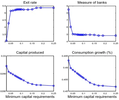
The intuition for the result is as follows. At low levels of the bank equity capital
require-ments, banks raise funds from depositors to exploit the subsidy implicit in government
bailouts. Banks, therefore, can provide more credit to capital-producing firms, which
re-sults in more capital being produced (bottom left panel of Fig. 4). More capital produced
means that growth is higher (bottom right panel of Fig.4). Higher growth normally would
promote welfare. However, as is clear from equation (1.23), growth is not the whole story;
the starting point of growth is no less important. At low levels of the bank equity capital
requirements, because banks have the default option and do not have enough “skin in the
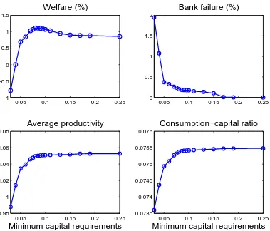
game,” they engage in risk-shifting, lending to risky-low-productivity firms. As a result, not
only is bank bankruptcy high (top right panel, Fig. 5), which leads to high capital losses,
average productivity is also low (top left panel of Fig. 5). Since investment is inefficient,
resources are left for consumption (bottom right panel, Fig. 5). The net effect is lower
welfare.
As the minimum capital constraint rises, the shadow cost of funds for banks becomes higher.
More banks exit because now private bank profitability is low (top left panel, Fig.4). As
a result, the total measure of banks is now lower (top right panel, Fig. 4). Consequently,
aggregate credit supply tightens, less capital is produced, and growth is lower. At the
same time, however, banks’ incentive for risk-shifting is also lower. Moreover, mandating
lower leverage through high capital requirements leads to lower bankruptcy rates (top right
panel, Fig.5) and hence less capital is lost due to default. The overall effect brings about
higher capital production productivity (bottom left panel of Fig.5) and higher consumption
(bottom right panel, Fig.5). This leads to an increase in welfare, which peaks at 1.1 percent
of lifetime consumption when the capital requirement is at 8%.
There are two reasons why requiring minimum equity capital higher than 8% leads to lower
welfare gains. The first is the equity flotation cost. Because banks must pay issuance costs
and since these costs are rebated back to households, the private cost of issuing equity
is higher than the social cost. Therefore, the funds that raised are lower than those in
a centralized economy. This leads to lower lending, lower capital production and hence
lower growth. The second reason is because of the presence of the “learning-by-doing”
spillover that is inherent in the Romer (1986) endogenous growth model. In this class of models, capital accumulation improves over all final good production productivity and
because this is external to each individual final good producer, decentralized allocations
entail under-investment and low capital accumulation. In the current setup, higher bank
capital requirements increases the cost of capital for banks, causing a reduction in lending
leading to low capital production and hence a lower accumulated capital stock. This brings
the decentralized allocations further away from the first-best allocation, and lowers welfare
1.4.4. Sensitivity Analysis
1.4.4.0.8 Role of probability of bailout λ. Fig. 6 plots the welfare analysis for a
higher level of bailout probability, increasing from 0.9 in the benchmark calibration to 0.95.
As expected, the welfare gain increases at the optimal level of capital requirement from 1.1%
to 1.8% of lifetime consumption, and the optimal minimum capital requirement increases
from 8% to 9%. This is intuitive since the likelihood of bailout is the source of distortions.
The more likely a bailout is, the more severe these distortions are, and so correcting these
distortions is more beneficial. Not only are welfare gains higher, the optimal level of the
minimum capital requirement is also higher. This is because the social cost of high bank
capital remains unchanged but the benefit of correcting distortions is now higher.
1.4.4.0.9 Role of equity issuance cost φ. Fig.7compares welfare results when there
is no equity issuance cost with the benchmark calibration. Not surprisingly the welfare
gains are higher in the case where equity issuance is costless. The result comes from the
fact that now the cost of funds for banks is lower, and as a consequence, relative to the
benchmark case, more funds are raised, more investment is undertaken, and more capital
is produced (right panel, Fig.7).
What is more interesting is that there is still a hump-shape in welfare as one varies the
minimum capital requiremente.¯ As discuss in subsection1.4.3, the hump-shape comes from
not only the issuance cost but also the under-investment in the decentralized allocations. As
more equity capital is required, banks can not exploit the implicit subsidy using deposits and
have to use a relatively more expensive form of funds from aprivate perspective; therefore,
equilibrium credit supply is lower, resulting in lower capital produced. Overall high capital
requirements still lead to lower welfare gains.
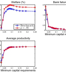
1.4.4.0.10 Role of productivity loss µ. Fig. 8 depicts welfare results for a lower µ
at .01 instead of .02 as in the benchmark case. Recall that µ is the average percentage
equilibrium outcome in two ways. On the one hand, lower µ leads to lower productivity
loss and makes investment more efficient. This tends to improve welfare.
On the other hand, lowerµencourages more banks to risk-shift, because now the private cost
of risk-shifting is lower due to ahigher productivity in risky-low-productivity firms relative
to the benchmark calibration. More risk-shifting by banks implies that more banks will
default relative to the benchmark (top right panel, Fig. 8). The net result is a reduction
in the average investment productivity (bottom panel). Hence, welfare is higher despite
lower productivity loss in risk-shifting (top left panel, Fig. 8). Moreover, the optimal level
of minimum bank capital requirement is now higher at 8.5%, attaining almost 1.5 percent
of lifetime consumption, while in the benchmark calibration the optimal level is 8%. This
result is due to the fact that in spite of lowerµ,the net negative effect of bank distortions is
higher (lower average productivity, Fig.8), and so the benefits of bank regulation is higher
while the cost of regulation has not changed.
1.4.4.0.11 Role of additional risk exposure σ. Fig. 9 compares welfare results in
the benchmark case with the case where the additional risk exposure due to risk-shifting
is higher. With higher risk exposure due to risk-shifting, the welfare gain is higher at the
optimal level of capital requirement, 1.35% versus 1.1%. Moreover, the optimal capital
ratio is also higher at 9% compared to 8% in the benchmark case. This is intuitive since the
upside potential of risk-shifting is higher, but the downside is unchanged, banks have more
incentives to risk-shift when risk exposure is higher. This leads to more capital losses due
to bank default and hence lowers investment productivity. Thus, from a social perspective,
the cost of risk-shifting is higher, and so is the benefit of higher bank capital requirements.
Since the cost of regulating banks is the same, this results in higher welfare gains and higher
1.5. Conclusion
This paper quantitatively studies the welfare implications of bank capital requirements in a
dynamic general equilibrium banking model. In the proposed model, because of government
bailouts, banks have incentives to risk-shift, leading to inefficient lending to
risky-low-productivity firms. Bank capital requirements reduce risk-shifting incentives and improve
welfare. The calibrated version of the model suggests that an 8% minimum Tier 1 capital
requirement brings about a significant welfare improvement of 1.1% of lifetime consumption.
This capital requirement is 2 percentage points higher than the level under Basel III and
current U.S. regulation. Moreover, from a social perspective, the bank cost of equity in this
model is not expensive. Welfare gains remain sizable even at a 25 percent minimum capital
requirement. Overall, my results highlight the need to re-examine current bank capital
regulations.
Further research should consider the impact of aggregate uncertainty on the optimal level of
minimum capital requirement as well as welfare implications of countercyclical bank capital
requirements policies. Moreover, the roles of other externalities such as contagious bank
failures and asset fire sale, should be analyzed. Intuition suggests that these externalities
would further strengthen the benefit of bank capital regulation now that the social cost of
bank failure is higher. The optimal level of capital ratio would therefore be even higher
−0.5 0 0.5 1 0
0.2 0.4 0.6 0.8 1
Exit decision
−0.5 0 0.5 1
0 0.5 1 1.5 2
Risk−shifting
−0.5 0 0.5 1
0 0.2 0.4 0.6 0.8 1
Net cash
Deposit−asset ratio
−0.5 0 0.5 1
−1 −0.5 0 0.5 1 1.5
Net cash
Equity payout−asset ratio
Figure 1: Policy functions: risk-shifting
−0.5 0 0.5 1 0
0.2 0.4 0.6 0.8 1
Exit decision
−0.5 0 0.5 1
−1 −0.5 0 0.5 1
Risk−shifting
−0.5 0 0.5 1
0 0.2 0.4 0.6 0.8 1
Net cash
Deposit−asset ratio
−0.5 0 0.5 1
−1 −0.5 0 0.5 1 1.5
Net cash
Equity payout−asset ratio
Figure 2: Policy functions: no risk-shifting
0.04 0.06 0.08 0.1 0.12 0.14 0.16 0.18 0.2 0.22 0.24 −0.8
−0.6 −0.4 −0.2 0 0.2 0.4 0.6 0.8 1 1.2
Welfare (%)
Minimum capital requirements
Figure 3: Welfare benefits
Notes – This figure shows the welfare result as a function of the minimum capital requirement e¯
0.05 0.1 0.15 0.2 0.25 3
3.5 4 4.5 5 5.5
Exit rate
0.05 0.1 0.15 0.2 0.25
4 5 6 7 8 9
Measure of banks
0.05 0.1 0.15 0.2 0.25
0.0298 0.0299 0.03
Capital produced
Minimum capital requirements
0.05 0.1 0.15 0.2 0.25
0.48 0.485 0.49 0.495
Consumption growth (%)
Minimum capital requirements
Figure 4: Consumption growth and distribution of banks
Notes – This figure shows exit rate, the measure of banks, capital produced and consumption growth as a function of the minimum capital requirement¯e. All other parameters are calibrated as in Table
0.05 0.1 0.15 0.2 0.25 −1
−0.5 0 0.5 1 1.5
Welfare (%)
0.05 0.1 0.15 0.2 0.25
0 0.5 1 1.5 2
Bank failure (%)
0.05 0.1 0.15 0.2 0.25
0.98 1 1.02 1.04 1.06 1.08
Average productivity
Minimum capital requirements
0.05 0.1 0.15 0.2 0.25
0.0735 0.074 0.0745 0.075 0.0755 0.076
Consumption−capital ratio
Minimum capital requirements
Figure 5: Welfare benefits, consumption and productivity
Notes – This figure shows the welfare result as a function of the minimum capital requirement e¯
0.04 0.06 0.08 0.1 0.12 0.14 0.16 0.18 0.2 0.22 0.24 −1.5
−1 −0.5 0 0.5 1 1.5 2
Welfare (%)
Minimum capital requirements
Benchmark
λ=.95
Figure 6: Role of probability of bailout λ
Notes – This figure shows the welfare result as a function of the minimum capital requirement e¯
0.05 0.1 0.15 0.2 0.25 −1
−0.5 0 0.5 1 1.5
Welfare (%)
Minimum capital requirements
Benchmark
φ= 0
0.05 0.1 0.15 0.2 0.25 0.0297
0.0298 0.0299 0.03
Capital produced
Minimum capital requirements
Figure 7: Role of equity issuance cost φ
Notes – This figure shows the welfare result as a function of the minimum capital requirement e¯
0.05 0.1 0.15 0.2 0.25 −1
−0.5 0 0.5 1 1.5
Welfare (%)
Benchmark
µ=.01
0.05 0.1 0.15 0.2 0.25 0
0.5 1 1.5 2 2.5
Bank failure (%)
Minimum capital requirements
0.05 0.1 0.15 0.2 0.25 0.96
0.98 1 1.02 1.04 1.06 1.08
Average productivity
Minimum capital requirements
Figure 8: Role of productivity loss due to risk-shifting µ
Notes – This figure shows the welfare result as a function of the minimum capital requirement e¯
0.04 0.06 0.08 0.1 0.12 0.14 0.16 0.18 0.2 0.22 0.24 −1
−0.5 0 0.5 1 1.5
Welfare (%)
Minimum capital requirements
Benchmark
σ²=.37
Figure 9: Role of additional risk exposure due to risk-shifting σ
Notes – This figure shows the welfare result as a function of the minimum capital requirement e¯
relative to the benchmark calibration with e¯=.04. Welfare is expressed in lifetime consumption units. The blue-circle line is welfare in the benchmark case (σ =.363), and the red-square line is
for the case with σ =.37. All other parameters are as calibrated in Table3. The x-axis indicates
CHAPTER 2 : Fiscal Policy and the Distribution of Consumption Risk
Mariano Massimiliano Croce and Thien T. Nguyen and Lukas Schmid
Abstract
This paper studies fiscal policy design in an economy in which endogenous growth risk and
asset prices are a first-order concern. When (i) the representative household has recursive
preferences, and (ii) growth is endogenously sustained through R&D investment, fiscal
policy alters both the composition of intertemporal consumption risk and the incentives to
innovate. Tax policies aimed at short-run stabilization may substantially increase long run
tax and growth risks and reduce both average growth and welfare. In contrast, policies
oriented toward asset price stabilization increase growth, wealth and welfare by lowering