113
Rainfall Forecast with Best and Full Members of the North American
Multi-Model Ensemble
Defi Yusti Faidah1,2a, Heri Kuswanto2b*, Suhartono2c & Kiki Ferawati2d
1 Department of Statistics, Faculty of Mathematics and Natural Sciences, Universitas Padjadjaran, Jalan Raya
Bandung-Sumedang Km.21, Jatinangor, 45363, Bandung-Sumedang, INDONESIA. E-mail: [email protected]
2 Department of Statistics, Faculty of Mathematics, Computation, and Data Science, Institut Teknologi Sepuluh
Nopember, Sukolilo, Surabaya, INDONESIA. E-mail: [email protected] ; [email protected]c ;
* Corresponding Author: [email protected]
Received: 21st April 2019 Revised : 6th August 2019 Published : 30th September 2019
DOI : https://doi.org/10.22452/mjs.sp2019no2.10
ABSTRACT The North American Multi-Model Ensemble (NMME) is a multi-model seasonal forecasting system consisting of models from combined US modelling centres. The NMME is expected to generate better rainfall prediction than a single model. However, the NMME forecasts are underdispersive or overdispersive, and calibration is needed to produce more accurate forecasting. This research examined the monthly rainfall data in Surabaya generated by nine NMME models and further calibrated them with bayesian model averaging (BMA). The purpose of this research was to assess the performance of the calibration results using the best four models and the full ensemble. The four models are CanCM3, CanCM4, CCSM3, and CCSM4, which were selected based on their skills. Both calibration results were evaluated using the continuous range probability score (CRPS) and the percentage of captured observations. The calibration with four models produced an average CRPS of 6.27 with 88.16% coverage, while with nine models an average CRPS of 5.23 with 92.11% coverage was obtained. This result suggests using the full ensemble to generate more accurate probabilistic forecasts.
Keywords: BMA, calibration, NMME
1. INTRODUCTION
The North American Multi-Model Ensemble (NMME) is a multi-model seasonal forecasting system consisting of coupled models from US modelling centres, including the NOAA National Centers for Environmental Prediction (NOAA/NCEP), the Center for Ocean-Land-Atmosphere Studies (COLA), the NOAA’s Geophysical Fluid Dynamics Laboratory (NOAA/GFDL), the National Aeronautics and Space Administration/Global Modeling and Assimilation Office (NASA/GMAO), and Canadian modelling centres (Kirtman et al., 2014). Becker et al. (2014) examined the
NMME’s skill and verified it against observations globally. They found that, for the precipitation rate and sea surface temperature, the NMME’s skill is higher than that of any single model, although there may be many regional and seasonal variations. The NMME usually makes better predictions than most, if not all, individual models. However, both the potential predictability and the real forecast skill vary depending on the geographical region and season.
114
scale. The second defines the most appropriate forecast parameters. Forecasting is performed every mid-month. Kirtman et al. (2014) explained that the multi-model approach using the NMME is more accurate than single-model forecasting. The NMME has been used extensively in previous research to verify forecasting results from the average monthly rainfall (Kuswanto, 2010; Wang et al., 2016), regional temperatures at 2 m above sea level (Becker et al., 2014), the sea surface temperature (Barnston et al., 2011; Kuswanto & Sari, 2013), seasonal rainfall (Ma et al., 2015), and seasonal droughts (Yuan & Wood, 2013).
A lot of researches showed that ensemble prediction systems have bias and hence, they have to be post-processed statistically to generate calibrated predictive distributions (Hamill & Colucci, 1997). Raftery et al. (2005) introduced Bayesian Model Averaging (BMA) with more recent extensions to quantitative precipitation (Sloughter et al., 2010), wind direction (Bao et al., 2013), and wind speed (Hamill & Colucci, 1997). The NMME’s skill has never been investigated. This research has several goals. The first is to show that the NMME has bias. The second is to verify that BMA can improve the reliability and validity of the NMME. The last is to assess the performance of calibration results using the best four models and the full ensemble evaluated using the continuous range probability score (CRPS) and the percentage of captured observations in Surabaya.
2. LITERATURE REVIEW
2.1 North American Multi-Model
Ensemble (NMME)
The NMME is a forecasting system consisting of coupled models from US and
Canadian modelling centres. The NMME was launched in the United States (Kirtman et al., 2014) with real-time experimental operational forecasts from the NOAA or the NCEP. The multi-model ensemble approach has been shown to produce better prediction quality on average than any single model of the ensemble, motivating the NMME’s undertaking (Doblas-Rayes et al., 2005; Gneiting et al., 2005; Hagedorn et al., 2004; Palmer, 2001; Smith et al., 2013). The models included in the NMME are CMC1-CanCM3 and CMC2-CanCM4 from CanSIPS, COLA-RSMAS-CCSM3 and COLA-RSMAS-CCSM4 from COLA, GFDL-CM2p1-aer04 from GFDL, ECHAM4p5-Anomaly and ECHAM4p5-DirectCoupled from IRI, and CFSv1 and CFSv2 from NCEP.
2.2 Bayesian Model Averaging (BMA)
Ensembles of numerical weather prediction models have been developed, in which multiple estimates of the current state of the atmosphere are used to generate probabilistic forecasts for future weather events. However, ensemble systems are uncalibrated and biased and thus need to be post-processed statistically, for which BMA is the preferred method. BMA was introduced by Raftery et al. (2005). The basic idea is that, for any given forecast ensemble, there is a best model or member, but we do not know which it is. In BMA, the overall forecast probability density function (pdf) is a weighted average of the forecast pdfs based on each of the individual forecasts. The weights are the estimated posterior model probabilities and reflect the models’ forecast skill. The forecast
k
f is then associated with a conditional pdf
|
k k
g y f , which can be interpreted as the
conditional pdf of y conditional on fk, given that fk is the best forecast in the ensemble. The BMA predictive model is:
1 1
1
| , , , |
K
K k k k
k
p y f f f w g y f
115
where fk is an ensemble forecast from K
models. wk is the posterior probability of forecast k being the best one. The wk’s are
probabilities, so they are non-negative and add up to 1. gk
y f| k
is the gamma pdf with meank k k
and standard deviation k k k , where k is the shape parameter andk is the
scale parameter. Thus, gk
y f| k
can bewritten as follows:
11
| ak exp
k k k
k k k
y
g y f y
a
(2)
2.3 Continuous Range Probability Score (CRPS)
The calibrated ensemble generates estimated intervals in pdf form. The CRPS is a much-used measure of performance for
probabilistic forecasts (Hersbach, 2000). It is derived from a quadratic measure of the difference between the forecast cumulative distribution function (cdf) and the empirical cdf of the observation. The formula of the CRPS can be written as follows:
0
21
1
( ) ( ) n
f
i i
f i x
CRPS F x F x dx
n
(3)where f( )
i
F x is the cdf from the forecast in the i-th period, 0( )
i
F x is the cdf from the observations
in the i-th period, and nf is the number of forecasts.
3. DATA AND METHODOLOGY
The data set used in this paper contains the monthly series of precipitation predictions from each individual model, which were downloaded from the official website of the NMME and the official website of the European Centre for Medium Range Weather Forecast (ECMWF). The data consist of monthly rainfall forecast results and the observed total rainfall in Juanda Surabaya. The two data sets have the same time periods, from 2003 to 2010. There are nine ensemble members, which are analysed as follows:
1. Evaluating the forecast model in the NMME data set against the real-time observations in the ECMWF data set using Root Mean Square Error (RMSE).
2. Calibrating the forecast models in the NMME data set with pre-process result data using the BMA approach. The calibration process using BMA will be examined for the window time (m) m12. The window time is the amount of data used to estimate the BMA parameters. The calibration is carried out in the following steps:
Starting a regression between forecasts as a predictor with the observation (dependent variable) using as many data as in the m -period before the calibrated period to obtain bias correction. Based on equation (3), estimating
116
algorithm. wk is the posterior probability of forecast k being the best one.
After all the parameters have been obtained, then the calibrated forecast can be obtained.
3. Evaluating the model’s reliability using the CRPS.
4. RESULT
4.1 Evaluation of the Rainfall Forecast Model
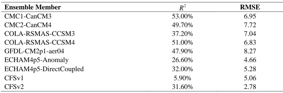
There are nine models to be calibrated in this research. However, they must be evaluated first to determine whether the individual models are reliable or not. In this research, the performance of the ensemble model is assessed using the R2 to determine the accuracy of the forecast in relation to the observations. In addition, the RMSE is used to evaluate the goodness of the model. Table 1 presents the performance of the monthly precipitation in individual models based on the
2
R and RMSE.
Table 1: Performance of monthly precipitation individual models.
Ensemble Member 2
R RMSE
CMC1-CanCM3 53.00% 6.95
CMC2-CanCM4 49.70% 7.72
COLA-RSMAS-CCSM3 37.20% 7.04
COLA-RSMAS-CCSM4 51.00% 6.83
GFDL-CM2p1-aer04 47.90% 8.27
ECHAM4p5-Anomaly 26.60% 4.66
ECHAM4p5-DirectCoupled 32.00% 5.28
CFSv1 5.90% 5.06
CFSv2 31.60% 2.78
Based on the values in Table 1, the best ensemble members are determined by comparing the R2value of each ensemble member with the observation data. The best are CMC1-CanCM3, CMC2-CanCM4, COLA-RSMAS-CCSM3, and COLA-RSMAS-CCSM3. CFSv2 has the smallest RMSE. The best model is selected using the R2 due to the fact that the basic idea of BMA is to capture the uncertainty. The R2 is used to explain how much variability in the observations that can be explained by the ensemble forecasting from each model.
4.2 Calibration of Rainfall Forecasts
117
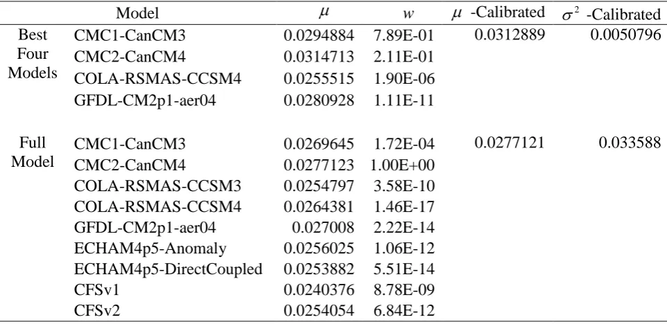
Table 2: BMA Parameters at -7o South and 113o East.
Model w -Calibrated 2
-Calibrated Best
Four Models
CMC1-CanCM3 0.0294884 7.89E-01 0.0312889 0.0050796 CMC2-CanCM4 0.0314713 2.11E-01
COLA-RSMAS-CCSM4 0.0255515 1.90E-06 GFDL-CM2p1-aer04 0.0280928 1.11E-11
Full
Model
CMC1-CanCM3 0.0269645 1.72E-04 0.0277121 0.033588 CMC2-CanCM4 0.0277123 1.00E+00
COLA-RSMAS-CCSM3 0.0254797 3.58E-10 COLA-RSMAS-CCSM4 0.0264381 1.46E-17 GFDL-CM2p1-aer04 0.027008 2.22E-14 ECHAM4p5-Anomaly 0.0256025 1.06E-12 ECHAM4p5-DirectCoupled 0.0253882 5.51E-14 CFSv1 0.0240376 8.78E-09 CFSv2 0.0254054 6.84E-12
Based on Table 2, CMC1-CanCM3 has the largest weight of the best four models, 7.89E-01. CMC2-CanCM4, COLA-RSMAS-CCSM4, and GFDL-CM2p1-aer04 have weights of 0.211, 0.0000019, and 1.11E-11. This means that CMC1-CanCM3 makes a greater contribution to BMA, because its weight is larger than the others. On the
contrary, COLA-RSMAS-CCSM4 and GFDL-CM2p1-aer04 do not contribute to BMA, because their weight is very small, while CMC2-CanCM4 has the largest weight in the full model and tends to be close to one. The larger weight indicates a greater contribution to BMA.
(a) (b)
Figure 1: BMA predictive pdf: (a) best four models; (b) full model.
Figure 1 shows the BMA forecasting results using the best four models and the full model. The orange vertical line indicates the observation data, and the black vertical line is the 95% confidence interval from the calibrated forecasting result. Based on Figure
118
precision is better. The full model’s pdf looks wider than that of the four models. This further shows the advantage of BMA, which can reduce underdispersiveness by attempting to adjust the variance, still covering the value of the observations.
4.3 CRPS Mean Value and Percentage of Captured Observations for Calibrated Forecasts using BMA
The purpose of the model evaluation is to determine which calibration method can provide better forecasting results, regarding both accuracy and density. The evaluation indicator uses the CRPS to compare the cdf between forecasting results and observation data. In addition, the evaluation of the calibrated forecast is assessed using the percentage of the captured observations. The CRPS and percentage of captured observations are shown in Table 3.
Table 3: CRPS Mean Value and Percentage of Captured Observations.
CRPS Percentage of Captured Observations
Best Four Models 6.27 88.16%
Full Model 5.23 92.11%
Table 3 shows that the full model has a smaller CRPS than the best four models. This indicates that the full model’s forecasting results will tend to have better reliability and density and be closer to the observation values. In addition, the percentage of captured observations by the interval calibrated full model is higher than that of the best four models.
5. CONCLUSION
Based on the analysis, it can be concluded that the accuracy model of the best four models produces an average CRPS of 6.27 with 88.16% coverage, while with nine models an average CRPS of 5.23 with 92.11% coverage is obtained. This result suggests using all the ensemble members in order to generate more accurate probabilistic forecasts.
6. REFERENCES
Barnston, A.G., Tippett, M.K., L’Heureux, M.L., Li, S. and DeWitt, D.G. (2011). Skill of real-time seasonal ENSO model predictions during 2002–11: Is our capability increasing?. Bulletin of the
American Meteorological Society, 93: 631-651.
Bao, L., Gneiting, T., Grimit, E.P., Guttorp, P. & Raftery, A.E. (2013). Bias correction and bayesian model averaging for ensemble forecasts of surface wind direction. Monthly Weather Review, 138: 1811-1821.
Becker, E., Van den Dool, D. & Zhang, Q. (2014). Predictability and forecast skill in NMME. Journal of Climate, 27(15): 5891-5906.
Doblas-Reyes, F.J., Hagedorn, R. & Palmer, T.N. (2005). The rationale behind the success of multi-model ensembles in seasonal forecasting-II calibration and combination. Tellus A, 57: 234-252.
Gneiting, T., Raftery, A.E., Westveld III, A.H. & Goldman, T. (2005). Calibrated probabilistic forecasting using ensemble model output statistics and minimum CRPS estimation. Monthly Weather Review, 135(5): 1098-1118.
119
success of multi-model ensembles in seasonal forecasting. Tellus A, 57: 219-233.
Hamill, T.M. & Colucci, S.J. (1997). Verification of Eta-RSM short-range ensemble forecast. Monthly Weather Forecast, 125: 1312-1327.
Hersbach, H. (2000). Decomposition of the continuous ranked probability score for ensemble prediction systems. Weather and Forecasting, 15: 59-570.
Kirtman, B.P., Min, D., Infanti, J.M., Kinter, J.L., Paolino, D.A., Zhang, Q. & Wood, E.F. (2014). The North American Multi Model Ensemble (NMME); Phase-1, Seasonal-to- Interannual Prediction; Phase-2, toward Developing Intraseasonal Prediction. Bulletin of the American Meteorological Society, 95(4): 585-601.
Kuswanto, H. (2010). New calibration method for ensemble forecast of non-normally distributed climate variables using meta-gaussian distribution. In: Chaerun, S.K. & Ihsanawati. (eds.): Science for Sustainable Development, Proceeding of the Third International Conference on Mathematics and Natural Sciences, Bandung, 23-25 November, pp. 932-939.
Kuswanto, H. & Sari, M.R. (2013). Bayesian model averaging with markov chain monte carlo for calibrating temperature forecast from combination of time series model.
Journal of Mathematics and Statistics,
9(4): 349-356.
Ma, F., Ye, A., Deng, X., Zhou, Z., Liu, X., Duan, Q. & Gong, W. (2015). Evaluating the skill of NMME seasonal precipitation ensemble predictions for 17 hydroclimatic regions in continental China. International Journal of Climatology, 36(1): 132-144.
Palmer, T.N.A. (2001). Nonlinear dynamical perspective on model error: a proposal for nonlocal stochastic–dynamic parameterization in weather and climate prediction models. Journal Meteorological Society, 127: 685-708.
Raftery, A.E., Gneiting, T., Balabdoul, F. & Polakowski, M. (2005). Using bayesian model averaging to calibrate forecast ensembles. Monthly Weather Review, 133: 1155-1174.
Sloughter, J.M., Gneiting, T., Raftery, A.E. (2010). Probabilistic wind speed forecasting using ensembels and bayesian model averaging. Journal of the American Statistical Association, 105(489): 25-35.
Smith, D.M., Scaife, A.A., Boer, G.J., Caian, M., Doblas-Reyes, F.J., Guemas, V. & Wyser, K. (2013). Real-time multi-model decadal climate predictions. Climate Dynamic, 41: 2875-2888.
Wang, S., Zhang, N., Wu, L. & Wang, Y. (2016). Wind speed forecasting based on the hybrid ensemble empirical mode decomposition and GA-BP neural network method. Renew Energy, 94: 629-36.