KEY GAME INDICATORS IN NBA PLAYERS’
PERFORMANCE PROFILES
Rubén Dehesa
1, Alejandro Vaquera
1,4, Bruno Gonçalves
2,3, Nuno Mateus
2,3,
Miguel-Ángel Gomez-Ruano
5, and Jaime Sampaio
2,31
VALFIS Research Group (IBIOMED), FCAFD, University of León, León, Spain
2Research Center in Sports Sciences, Health Sciences and Human Development, CIDESD,
CreativeLab Research Community, Vila Real, Portugal
3University of Trás-os-Montes e Alto Douro, Vila Real, Portugal
4
Institute of Sport & Exercise Science, University of Worcester, Henwick Grove,
Worcester, United Kingdom
5
Universidad Politécnica de Madrid, Spain
Original scientific paper https://doi.org/10.26582/k.51.1.9
Abstract:
The aim of the present study was to identify and describe players’ performances in NBA games using individual and team-based game variables. The sample was composed of 535 balanced games (score differences below or equal to eight points) from the regular season (n=502) and the playoffs (n=33). A total of 472 players were analysed. The individual-based variables were: minutes on court, effective field-goal percentage, free-throws/field-goals ratio, offensive rebound percentage, turnover percentage and playing position. The team-based variables were: team points minus opponent’s points (on and off court), NET score (player’s on values minus his off values), maximum negative and positive point difference, team’s winning percentage, game pace, defensive and offensive ratings. A two-step cluster analysis was performed to identify player’s profiles during regular season and playoff games. The results identified five performance profiles during regular season games and four performance profiles during playoff games. The profiles identified were mainly characterized by the game quarter and the negative NET indicator (players’ performance on court minus their performance off court) in the regular season games and the positive NET indicator during the playoff games and the second and third game-quarters. Coaching staffs can fine-tune these profiles to develop more team-specific models and, conversely, use the results to monitor and rebuild team formation under the constrained dynamics of the game and competition stages.
Key words:collective behaviour, decision-making, game statistics, machine learning, cluster analysis, elite basketball
Introduction
The National Basketball Association (NBA) is the most worldwide competitive basketball league. The competition is extremely congested requiring multidisciplinary approaches to provide accurate information about players and teams’ performance over the season. Therefore, contemporary basket-ball performance analysis demands from players
and teams the combination of physical fitness profiles (Gonzalez, et al., 2013) with technical and
tactical indicators (Mangine, et al., 2014) during the season.
Within this research approach, the computer vision systems have provided a great support in
performance indicators such as the effective field goal percentage (eFG%), the turnover percentage (TOV%), the offensive and defensive rebound percentage (ORB%, DRB%, respectively) and
the free-throw factor (FT) obtained by dividing
the free-throw attempts by the field goal attempts
(Oliver, 2004).
The basketball research has been focused on the
identification of possible key performance indica -tors (KPIs) that might allow obtaining performance information from players and teams. However, despite the analysis of KPIs, there is a need to explore other variables such as the team points minus the
opponents’ points when a specific player was on the floor (described as ON), the team points minus the opponents’ points when the specific player was off the floor (described as OFF), or the difference
between ON and OFF (described as NET). In fact, these novel variables may provide a step forward in understanding on how game-related statistics may help to functionally evaluate technical and tactical behaviour of players and teams. In addition, the insights by dynamic and self-organized perspec-tives aiming to understand emergent behaviours
(Bourbousson, Seve, & McGarry, 2010; Esteves, et
al., 2016; Leite, et al., 2014) suggest that the entire basketball team’s behaviour is widely depended on how a player interacts with his/her teammates, the opponents and the game context. Indeed, basketball may be the arduous game to characterize individual players’ performance, since each one is critically
influenced by the other players on the court, of the
own and opposing team alike (Lutz, 2012). In addi-tion, recent analyses (Alagappan, 2012) had shown that the traditional method of clustering players’ court-position could be terribly misleading and somewhat obsolete. Thus, this additional informa-tion may be useful for coaches when considering the decisions taken during game critical moments such as substitutions or changes in the team’s strategy; and can also be a key-factor on general managers’ approaches when it comes the time to build the team’ roster.
During game dynamics there are several stra-tegic decisions that constrain the player’s behav-iours such as the players’ characteristics, the task and the environment (Newell & Ranganathan, 2010). The physiological, tactical, and game-related indicators appear as examples of factors that are well related to the behavioural changes across game
quarters (Gomez, Lorenzo, Ibanez, & Sampaio,
2013; Scanlan, et al., 2015). Also, it seems
predict-able that specific playing positions may provide
dissimilarities in how the game and player interac-tions change over the course of time.
Conversely, the players’ positioning varia-bles allow exploring and a better understanding of players’ performance. For example, Sampaio
NBA all-star and non-all-star players and suggested that the all-star players recognized and perceived environmental information more easily and effec-tively. In addition, Mateus et al. (2015) added that high variability in performance might be related to performing poorly in NBA games. The authors argued that players from losing teams had greater variability in defensive and offensive statistics, particularly in away games and of players who played longer durations.
Considering the presented state of the art, this study aims to identify and describe different
basket-ball game performance profiles in NBA regular
season and playoffs using new combined tracking and notational-based variables.
Methods
Sample and variables
Archival data were obtained from the publicly
accessible official NBA records (available at www. nba.com and www.basketball-reference.com) for 1,311 games played during the 2014/2015 season. Sample included 502 games from the regular season and 33 games from the playoffs and a total of 472
and analysed, since only balanced games (final
score differences below or equal to eight points) were considered (Sampaio, Lago, Casais, & Leite, 2010). The games that ended with overtimes were also excluded as well as the players that
partici-pated less than five minutes in any game (Sampaio,
Janeira, Ibanez, & Lorenzo, 2006). The variables analysed included individual and collective actions
and were defined as follows:
• ON: Plus/minus (Team Points minus Opponent Points) when the player was on the court. • OFF: Plus/minus (Team Points minus
Oppo-nent Points) when the player was off the court. • NET: Difference between ON and OFF. • MAX NEG (Maximum Negative Points Differ
-ence): High negative points difference in the periods when the player was on the court. • MAX POS (Maximum Positive Points
Differ-ence): High positive points difference in the periods when the player was on the court. • Time: Minutes on the court (per player). • Team Wins: Winning percentage.
• Pace: an estimate of the number of posses-sions per 48 minutes by a team. The computing formula is (Oliver, 2004):
4 · [(Team Possession + Opponent Possession) / (2 · Team Minutes Played / 5)]
• DRtg (Defensive Rating): Team points conceded per 100 possessions (Oliver, 2004).
• ORtg (Offensive Rating): Team points scored per 100 possessions (Oliver, 2004).
• eFG% (Effective Field Goal Percentage): Statis
goal. The computing formula is (Oliver, 2004):
(Field Goals + 0.5 · 3-Point Field Goals) / Field Goal Attempts.
• FT/FGA (Oliver, 2004): Free Throws / Field Goal Attempts.
• ORB% (Offensive Rebound Percentage): An
estimate of the percentage of available offensive rebounds a player grabbed while he was on the court. The computing formula is (Oliver, 2004): 100 · [Offensive Rebounds · (Team Minutes Played / 5)] / [Minutes Played · (Team Offensive Rebounds + Opponent Defensive Rebounds)]. • TOV% (Turnover Percentage): An estimate of
turnovers per 100 plays. The computing formula is (Oliver, 2004):
100 · Turnovers / (Field Goal Attempts + 0.44
· Free Throw Attempts + Turnovers).
Data analysis
The regular season and the playoff databases were analysed separately. Firstly, maximally
different clusters were identified by the following variables: ON, OFF, NET, MAX NEG, MAX POS, ON concerning the first quarter (1Q), 2Q, 3Q and 4Q. Therefore, a two-step cluster with log-like -lihood as the distance measure and Schwartz’s Bayesian criterion was performed to classify the players’ performances. This method differs from the traditional clustering techniques by automati-cally determining the optimal number of clusters and scalability (Tabachnick & Fidell, 2007). The variables were ranked according to the predic-tor’s importance, providing normalized weights to support the cluster distribution, and computed the percentage that each player appeared in the obtained clusters. Secondly, the clusters were differentiated using the one-way analysis of variance for numer-ical variables (KPIs). The Bonferroni post-hoc
tests were carried out when necessary to establish comparisons among the groups. Effects sizes (ES)
were calculated (eta squared, η2) to show the
magni-tude of the effects and their interpretation was based on the following criteria: 0-.1=weak, .1-.3=modest, .3-.5=moderate, >.5=strong (Cohen, 1988). Finally, a crosstab command (Pearson’s Chi-square test) was used to differentiate the categorical variables (team wins and playing positions) among the clus-ters during regular season and playoff games. Effect sizes (ES) were calculated using the Cramer’s V test and their interpretation was based on the following criteria: .10=small effect, .30=medium effect, and .50=large effect (Volker, 2006). The statistical anal-yses were done using the SPSS software (IBM SPSS Statistics for Windows, Version 21.0. Armonk, NY:
IBM Corp.). The level of significance was set at
p<.05.
Results
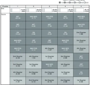
Figure 1 presents the cluster analysis solu-tion obtained for the regular season games. The colour density refers to the overall predictor impor-tance, whereas the inputs are sorted by the
within-cluster importance. The model is constituted by five
different clusters ranging between 14.4 (cluster 1)
and 24.5% (cluster 2) of the sample. The
within-cluster predictor importance allows identifying
that performances from the first cluster are nega -tive (NET=-20.3±6.9), the team performed better when these players were not playing (OFF=9.8±4.8) and the most important quarters were the 2nd and
the 3rd one (see Figure 1).
Figure 2 presents the cluster analysis solution for the playoff games. The model is constituted by four different clusters ranging between 17.1
(cluster 2) and 34.5% (cluster 4) of the sample. The
within-cluster predictor importance was substan-tially different from the one obtained for the regular season games. For example, it allows identifying that performances from the second cluster are described by positive performances in the 2nd and
negative performances in the 3rd quarter (2Q=8.32 and 3Q=-5.78), although these players could main -tain a positive NET score (see Figure 2).
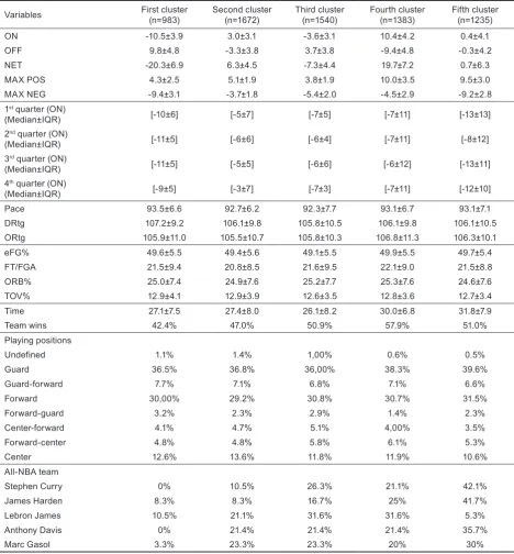
Table 1 and Table 2 present the performance descriptors for the cluster concerning game
quar-ters, team efficacy, team four factors, and team cluster-related variables for regular season and playoff games, respectively. Descriptions are complemented with the distribution of different performances by playing positions and by the players awarded by sportswriters and broadcasters
for the All-NBA first team.
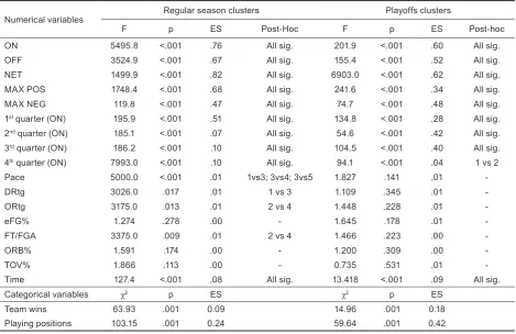
Table 3 includes the differences among the clus-ters for the regular season and the playoff games. During the regular season games, the variables that differentiated among clusters were: ON, MAX
POS, MAX NEG, 1Q, 2Q, 3Q and 4Q, NET, Pace, FT/FGA, ORtg, DRtg, time, team win, and playing
position.
In addition, the differentiating clusters found during the playoff games showed the importance of:
ON, MAX POS MAX NEG, 1Q, 2Q, 3Q and 4Q,
NET, team win, and playing position (see Table 3).
Discussion and conclusions
The present study aimed to identify and describe
different basketball game performance profiles in NBA regular season and playoff games. Generally,
Figure 2. Cluster analysis of the playoff´s dataFigure 1. Cluster analysis of the regular season’s data.
Figure 2. Cluster analysis of the playoff´s data
Table 1. Performance descriptors for the clusters identified in the regular season games
Variables First cluster(n=983) Second cluster(n=1672) Third cluster(n=1540) Fourth cluster(n=1383) Fifth cluster(n=1235)
ON -10.5±3.9 3.0±3.1 -3.6±3.1 10.4±4.2 0.4±4.1
OFF 9.8±4.8 -3.3±3.8 3.7±3.8 -9.4±4.8 -0.3±4.2
NET -20.3±6.9 6.3±4.5 -7.3±4.4 19.7±7.2 0.7±6.3
MAX POS 4.3±2.5 5.1±1.9 3.8±1.9 10.0±3.5 9.5±3.0
MAX NEG -9.4±3.1 -3.7±1.8 -5.4±2.0 -4.5±2.9 -9.2±2.8
1st quarter (ON)
(Median±IQR) [-10±6] [-5±7] [-7±5] [-7±11] [-13±13]
2nd quarter (ON)
(Median±IQR) [-11±5] [-6±6] [-6±4] [-7±11] [-8±12]
3rd quarter (ON)
(Median±IQR) [-11±5] [-5±5] [-6±6] [-6±12] [-13±11]
4th quarter (ON)
(Median±IQR) [-9±5] [-3±7] [-7±3] [-7±11] [-12±10]
Pace 93.5±6.6 92.7±6.2 92.3±7.7 93.1±6.7 93.1±7.1
DRtg 107.2±9.2 106.1±9.8 105.8±10.5 106.1±9.8 106.1±10.5
ORtg 105.9±11.0 105.5±10.7 105.8±10.3 106.8±11.3 106.3±10.1
eFG% 49.6±5.5 49.4±5.6 49.1±5.5 49.9±5.5 49.7±5.4
FT/FGA 21.5±9.4 20.8±8.5 21.6±9.5 22.1±9.0 21.5±8.8
ORB% 25.0±7.4 24.9±7.6 25.2±7.7 25.3±7.6 24.6±7.6
TOV% 12.9±4.1 12.9±3.9 12.6±3.5 12.8±3.6 12.7±3.4
Time 27.1±7.5 27.4±8.0 26.1±8.2 30.0±6.8 31.8±7.9
Team wins 42.4% 47.0% 50.9% 57.9% 51.0%
Playing positions
Undefined 1.1% 1.4% 1,00% 0.6% 0.5%
Guard 36.5% 36.8% 36,00% 38.3% 39.6%
Guard-forward 7.7% 7.1% 6.8% 7.1% 6.6%
Forward 30,00% 29.2% 30.8% 30.7% 31.5%
Forward-guard 3.2% 2.3% 2.9% 1.4% 2.3%
Center-forward 4.1% 4.7% 5.1% 4,00% 3.5%
Forward-center 4.8% 4.8% 5.8% 6.1% 5.3%
Center 12.6% 13.6% 11.8% 11.9% 10.6%
All-NBA team
Stephen Curry 0% 10.5% 26.3% 21.1% 42.1%
James Harden 8.3% 8.3% 16.7% 25% 41.7%
Lebron James 10.5% 21.1% 31.6% 31.6% 5.3%
Anthony Davis 0% 21.4% 21.4% 21.4% 35.7%
Marc Gasol 3.3% 23.3% 23.3% 20% 30%
Table 2. Performance descriptors for the clusters identified in the playoff performances
Variables First cluster (n=82) Second cluster (n=74) Third cluster (n=127) Fourth cluster (n=149)
ON 10.8±5.9 0.6±6.5 2.9±4.1 -6.7±5.3
OFF -9.1±5.6 -1.9±5.5 -3.1±5.3 6.3±5.5
NET 19.9±10.0 2.5±10.8 6.1±7.5 -13.0±9.4
MAX POS 10.4±2.5 9.8±3.8 4.6±2.1 4.7±2.7
MAX NEG -5.7±3.6 -8.1±2.9 -3.4±1.9 -8.0±3.0
1st quarter (ON)
(Median±IQR) [2±13] [-12±3] [-4±6] [-11±9]
2nd quarter (ON)
3rd quarter (ON)
(Median±IQR) [-4±14] [-10±0] [-4±4] [-5±5]
4th quarter (ON)
(Median±IQR) [-8±8] [-5±8] [-4±4] [-9±7]
Pace 93.5±4.3 94.6±4.7 93.4±3.3 94.1±3.9
DRtg 104.7±9.5 105.8±10.6 107.0±8.7 105.5±9.5
ORtg 106.5±9.6 104.5±10.3 106.9±8.8 105.0±9.5
eFG% 49.2±5.1 47.3±5.1 48.5±5.4 48.3±5.0
FT/FGA 21.6±8.6 23.9±9.0 23.0±8.6 21.8±8.5
ORB% 24.1±6.4 25.0±6.1 23.3±5.8 23.9±6.3
TOV% 12.0±3.8 11.9±3.0 11.5±3.2 12.1±3.7
Time 33.9±6.9 34.7±8.3 28.0±9.7 29.9±8.8
Team wins 67.1% 36.5% 48.8% 50.3%
Playing positions
Guard 36.6% 43.2% 34.6% 39.6%
Guard-forward 6.1% 1.4% 8.7% 9.4%
Forward 29.3% 32.4% 26.0% 29.5%
Forward-guard 4.9% 1.4% 6.3% 1.3%
Center-forward 2.4% 5.4% 11.0% 5.4%
Forward-center 2.4% 1.4% 4.7% 7.4%
Center 18.3% 14.9% 8.7% 7.4%
All-NBA team
Stephen Curry 33% 33% 0% 33%
James Harden 25% 25% 0% 50%
Lebron James 20% 30% 20% 30%
Anthony Davis 0% 0% 0% 100%
Marc Gasol 25% 25% 50% 0%
Table 3. Results of the differences among clusters using one-way analysis of variance (ANOVA) for numerical variables and crosstab’s command for nominal variables during the regular season and playoff games
Numerical variables Regular season clusters Playoffs clusters
F p ES Post-Hoc F p ES Post-hoc
ON 5495.8 <.001 .76 All sig. 201.9 <.001 .60 All sig.
OFF 3524.9 <.001 .67 All sig. 155.4 <.001 .52 All sig.
NET 1499.9 <.001 .82 All sig. 6903.0 <.001 .62 All sig.
MAX POS 1748.4 <.001 .68 All sig. 241.6 <.001 .34 All sig.
MAX NEG 119.8 <.001 .47 All sig. 74.7 <.001 .48 All sig.
1st quarter (ON) 195.9 <.001 .51 All sig. 134.8 <.001 .28 All sig.
2nd quarter (ON) 185.1 <.001 .07 All sig. 54.6 <.001 .42 All sig.
3rd quarter (ON) 186.2 <.001 .10 All sig. 104.5 <.001 .40 All sig.
4th quarter (ON) 7993.0 <.001 .10 All sig. 94.1 <.001 .04 1 vs 2
Pace 5000.0 <.001 .01 1vs3; 3vs4; 3vs5 1.827 .141 .01
-DRtg 3026.0 .017 .01 1 vs 3 1.109 .345 .01
-ORtg 3175.0 .013 .01 2 vs 4 1.448 .228 .01
-eFG% 1.274 .278 .00 - 1.645 .178 .01
-FT/FGA 3375.0 .009 .01 2 vs 4 1.466 .223 .00
-ORB% 1.591 .174 .00 - 1.200 .309 .00
-TOV% 1.866 .113 .00 - 0.735 .531 .01
-Time 127.4 <.001 .08 All sig. 13.418 <.001 .09 All sig.
Categorical variables χ2 p ES χ2 p ES
Regular season
In the regular season games, the cluster analysis
identified five different game performance profiles. The players from clusters one, two and five were mostly classified by their negative performance
records. The players from cluster one presented the poorest performances, as revealed by the higher number of turnovers and the worst defen-sive ranking, which may suggest poor ability and skills (Sampaio, Drinkwater, & Leite, 2010). This
individual performance had reflections in team’s
performance, since they were outscored when these
specific players were on the floor. Therefore, it is
not surprising that these players were the second group with less playing time (Sampaio, et al., 2010). As expected, the All-NBA team players were lesser concentrated in these cluster.
The players from clusters two and five were
also highly characterized by negative performance records; however, both presented good perfor-mances when they were on the court and their teams performed better. The results demonstrated a strong
relation with MAX NEG performance records,
however, they also revealed that both contributed positively to their teams. Moreover, both had some positive performance records in other variables, evidences that could be associated to less consist-ency in players’ performance during the game or to key players who were not able to overcome their poor performance periods. In fact, the players from cluster two showed differences among game quar-ters, by achieving great improvements in the 4th
quarter (Ferreira, Volossovitch, & Sampaio, 2014), suggesting that these players assumed a special role in the most decisive moments of the game. The players from the All-NBA team were mainly
allo-cated in cluster five, surprisingly displayed a drop in their performance from the first to the second
half, where normally the game is more balanced
and unpredictable (Gomez, Gasperi, & Lupo, 2016).
Then, despite being the all-star players, during the regular season their performance showed decreases and seemed affected by the game criticality (Beilock
& Gray, 2007; Wallace, Baumeister, & Vohs, 2005).
The players from cluster three showed a strong association with MAX POS variable; however, their teams displayed lower performances when they were on the court. These players presented
the lower playing time and the worst effective
field-goal percentage, despite belonging to the teams that had a positive percentage of wins. These evidences may suggest that the players from cluster three produce lower team’s performance when they are on court (Mateus, et al., 2015). Nonetheless, these players exhibited the best defensive scores. Thus, the coaches may pay attention to this evidence about the defensive role that they could accomplish.
Finally, the players from cluster four were cate-gorized by the best positive performance records, suggesting that they were important to their
teams. This finding justifies the team’s perfor -mance decreases when they were replaced during the game rotations. Moreover, they had the best winning percentage and shooting percentage from
the field. Then, it is not surprising that their playing
time was approximately 30 minutes per game since this information indicated that their quality is quite high (Sampaio, et al., 2010). Winston (2012) revealed that according to the four-factor model, good shooting teams tended to be poor offensive rebounding teams. Nonetheless, the players from
this cluster presented the highest effective field goal
percentage and the highest offensive rebounding percentage. These trends are likely associated with a better knowledge of the game and decision-making adapted to the environmental conditions (Sampaio, et al., 2015). These skills would allow players to assume properly positioning and secure the offensive rebound after a teammate has taken a
shot. General managers and coaching staffs could
be interested in recruiting players that present more games on this cluster, as they might repre-sent better adaptation to the environment and, ulti-mately, higher possibilities of being successfully integrated into a new team.
Playoffs
In the playoffs, the cluster analysis allowed discriminating four different groups of perfor-mances. Contrary to the performance achieved in the games of the regular season, the playoff groups differed mostly in the NET variable. Differences among the groups were once again noted in the different game quarters.
Similarly to the regular season games, the players who presented the higher ON positive
differ-ences and the higher effective field-goal percentage
did not played for longer durations, despite their teams demonstrated a breaking in scoring perfor-mance when they were on the bench. The NBA playoffs exposes the players’ performances to a highly congested schedule, and perhaps coaches decided to rest players from cluster one during the game, to improve their recovery (Sampaio, et al., 2010). This approach would prevent the impact of
fatigue on performance (Gabbett, 2008; Russell,
Benton, & Kingsley, 2011) and teams’ competitive ability (Montgomery, et al., 2008). In opposition to
the regular season findings, the largest concentra -tion of centres was presented in this cluster, perhaps because during the playoffs the teams look for easier and more effective strategies to achieve points (see
effective field-goal percentage) (Mateus, et al.,
participa-tion of players that normally conduct their
behav-iours near to the basket (Erčulj & Štrumbelj, 2015; Gomez, et al., 2016; Mateus, et al., 2018).
The players from cluster two exhibited the
lowest effective field-goal percentage and play in
the less successful teams (less wins). Neverthe-less, they lead the clusters in minutes per game. According to Sampaio et al. ( 2010), the most valu-able players tend to play more time, and perhaps during the playoffs the teams with players who played- longer were more dependent on them. Since teams are more dependent on such players, it is easier for the opponents to overturn them and their teams through special tactics (Mateus, et al., 2018).
These findings could be a reason for the players
from cluster two teams that presented minimal score differences, even when they were on the court. Moreover, this cluster was largely composed of guards, which corroborates the above-mentioned information that teams were more dependent on players from this cluster, since NBA guards had a leadership role in teams’ offensive patterns (Fewell, Armbruster, Ingraham, Petersen, & Waters, 2012). The players from cluster three played less minutes per game, despite having the lowest turn-overs percentage and the second best effective
field-goal percentage. Indeed, these players could
be important offensive threats or shooting special-ists (Mateus, et al., 2018). Additionally, their teams
outscored their opponents with them on the floor.
Perhaps, they were a typical six-man that comes off the bench as a strategy to try to change game dynamics (Sampaio, et al., 2010).
The players from cluster four were mostly
clas-sified by their negative performance records. These
players impaired their teams’ outcome when they were on the court, because the difference between the points scored and the points conceded was largely unfavourable, likely due to a poor
offen-sive efficiency and a higher turnover percentage
(Sampaio, et al., 2010). However, it is interesting to note that the all-NBA team power-forward and
shooting guard integrated this cluster (100 and 50%,
respectively), despite surely being the most valuable players of their teams.
Once again, the clusters displayed consider-able differences between the game quarters. For example, the players from cluster one presented the largest magnitude of NET values and belonged to the best teams, and exhibited the best score
differ-ences in the first quarters of each half. According
to Abdelkrim, El Fazaa and El Ati (2007), the game intensity is higher in these quarters. Since these players belong to the best teams, they are familiar with enhanced training environments (Sampaio, et al., 2010), and then, they can easily adapt to these conditions. Moreover, Sampaio et al. (2015) suggested that the best players
inter-was useful to select the appropriate opportuni-ties to decide and act (Davids, Araújo, Correia, & Vilar, 2013). Perhaps these players decide to play
at a higher game intensity in the first game quar -ters of each half (which increases their performance during these periods) with the intention to build an important score advantage. The worst perfor-mance in the fourth quarter was possibly because in the decisive quarter the game outcome was already decided and consequently the players’ intensity
and focus decreased (Moreno, Gomez, Lago, &
Sampaio, 2013), conducting to a less satisfactory and consistent performances (Sampaio, et al., 2010). The players from cluster two played longer in the playoffs and presented the greatest ON differ-ences in the second and fourth quarters of the game. Casals and Martinez (2013) stated that long
time-played could be a result of presenting higher influ -ence in all strategic planning and tactical responses of the team. This fact especially makes sense in the second quarter (e.g., if the coach’s intention was that the team went to the half-time with a more favour-able outcome). Another possible explanation could be that these players take longer to appear in the game, because they need more time to get familiar with the different environmental game constraints (Sampaio, et al., 2010). Their improvements in performance in the fourth quarter were also very relevant, because NBA players usually drop in higher pressure moments, such as the last game quarter of the playoffs games (Wallace, Caudill, & Mixon Jr., 2013).
In conclusion, this study allowed identifying
several different performance profiles of NBA
regular season and playoff games using novel
KPIs. Coaching staffs can fine-tune these profiles to develop more team-specific models and, conversely,
use the results to monitor and rebuild team consti-tution under the constrained dynamics of the game and competition stages (change the player rotation, restricting minutes of the players with a negative performance to the quarter where they perform better).
The main limitation of this study is the fact that it measured individual performance, which depends not only on the record of the team, but also on the teammates and opponents with whom each player is on the court. The best teams tend to have positive NET and worse players can be in favour when they play with the best player, while on the other hand, the best players of teams with
References
Abdelkrim, N.B., El Fazaa, S., & El Ati, J. (2007). Time-motion analysis and physiological data of elite under-19-year-old basketball players during competition. British Journal of Sports Medicine, 41(2), 69-75.
Alagappan, M. (2012). From 5 to 13: Redefining the positions in basketball. Paper presented at the 2012 MIT Sloan Sports Analytics Conference, Boston, MA, USA. Retrieved February 22, 2016 from: http://www.sloansportsconference. com/content/the-13-nba-positions-using-topology-to-identify-the-different-types-of-players/
Beilock, S.L., & Gray, R. (2007). Why do athletes choke under pressure? In G. Tenenbaum & R.C. Eklund (Eds.), Handbook of sport psychology (pp. 425-444). Hoboken, NJ: John Wiley & Sons.
Bourbousson, J., Seve, C., & McGarry, T. (2010). Space-time coordination dynamics in basketball: Part 1. Intra- and inter-couplings among player dyads. Journal of Sports Sciences, 28(3), 339-347. doi: 10.1080/02640410903503632 Bruce, S. (2016). A scalable framework for NBA player and team comparisons using player tracking data. Journal of
Sports Analytics, 2(2):107–119.
Casals, M., & Martinez, J.A. (2013). Modelling player performance in basketball through mixed models. International Journal of Performance Analysis in Sport, 13(1), 64-82.
Cohen, J. (1988). Statistical power analysis for the behavioral sciences. Hillsdale, NJ: Erlbaum Associates.
Davids, K., Araújo, D., Correia, V., & Vilar, L. (2013). How small-sided and conditioned games enhance acquisition of movement and decision-making skills. Exercise and Sport Sciences Reviews, 41(3), 154-161.
Erčulj, F., & Štrumbelj, E. (2015). Basketball shot types and shot success in different levels of competitive basketball. PLOS One, 10(6), e0128885.
Esteves, P.T., Silva, P., Vilar, L., Travassos, B., Duarte, R., Arede, J., & Sampaio, J. (2016). Space occupation near the basket shapes collective behaviours in youth basketball. Journal of Sports Sciences, 34(16), 1557-1563. doi: 10.1080/02640414.2015.1122825
Ferreira, A.P., Volossovitch, A., & Sampaio, J. (2014). Towards the game critical moments in basketball: A grounded theory approach. International Journal of Performance Analysis in Sport, 14(2), 428-442.
Fewell, J.H., Armbruster, D., Ingraham, J., Petersen, A., & Waters, J.S. (2012). Basketball teams as strategic networks.
PLOS One, 7(11), e47445.
Gabbett, T.J. (2008). Influence of fatigue on tackling technique in rugby league players. Journal of Strength and Conditioning Research, 22(2), 625-632. doi: 10.1519/JSC.0b013e3181635a6a
Gomez, M.A., Gasperi, L., & Lupo, C. (2016). Performance analysis of game dynamics during the 4th game quarter of NBA close games. International Journal of Performance Analysis in Sport, 16(1), 249-263.
Gomez, M.A., Lorenzo, A., Ibanez, S.J., & Sampaio, J. (2013). Ball possession effectiveness in men’s and women’s elite basketball according to situational variables in different game periods. Journal of Sports Sciences, 31(14), 1578-1587. doi: 10.1080/02640414.2013.792942
Gonzalez, A.M., Hoffman, J.R., Rogowski, J.P., Burgos, W., Manalo, E., Weise, K., . . ., & Stout, J.R. (2013). Performance changes in NBA basketball players vary in starters vs nonstarters over a competitive season. Journal of Strength and Conditioning Research, 27(3), 611-615. doi: 10.1519/JSC.0b013e31825dd2d9
Leite, N.M., Leser, R., Goncalves, B., Calleja-Gonzalez, J., Baca, A., & Sampaio, J. (2014). Effect of defensive pressure on movement behaviour during an under-18 basketball game. International Journal of Sports Medicine, 35(9), 743-748. doi: 10.1055/s-0033-1363237
Lutz, D. (2012). A cluster analysis of NBA players. Paper presented at the Proceedings of the MIT Sloan Sports Analytics Conference, Boston, MA, USA. Retrieved February 24, 2016 from: http://www.sloansportsconference.com/ wp-content/uploads/2012/02/44-Lutz_cluster_analysis_NBA.pdf
Maheswaran, R., Chang, Y., Henehan, A., & Danesis, S. (2012). Deconstructing the rebound with optical tracking data. Paper presented at the 2016 MIT Sloan Sports Analytics Conference, Boston, MA, USA. Retrieved February 27, 2016 from http://www.sloansportsconference.com/wp-content/uploads/2012/02/108-sloan-sports-2012-maheswaran-chang_updated.pdf
Mangine, G.T., Hoffman, J.R., Wells, A.J., Gonzalez, A.M., Rogowski, J.P., Townsend, J.R., . . ., & Stout, J.R. (2014). Visual tracking speed is related to basketball-specific measures of performance in NBA players. Journal of Strength and Conditioning Research, 28(9), 2406-2414. doi: 10.1519/jsc.0000000000000550
Mateus, N., Gonçalves, B., Abade, E., Leite, N., Gomez, M.A., & Sampaio, J. (2018). Exploring game performance in NBA playoffs. Kinesiology, 50(1), 89-96.
Mateus, N., Gonçalves, B., Abade, E., Liu, H., Torres-Ronda, L., Leite, N., & Sampaio, J. (2015). Game-to-game variability of technical and physical performance in NBA players. International Journal of Performance Analysis in Sport, 15(3), 764-776.
Mikolajec, K., Maszczyk, A., & Zajac, T. (2013). Game indicators determining sports performance in the NBA. Journal of Human Kinetics, 37, 145-151.
Moreno, E., Gomez, M.A., Lago, C., & Sampaio, J. (2013). Effects of starting quarter score, game location, and quality of opposition in quarter score in elite women’s basketball. Kinesiology, 45(1), 48-54.
Newell, K., & Ranganathan, R. (2010). Instructions as constraints in motor skill acquisition. In I. Renshaw, K. Davids, & G. Savelsbergh (Eds.), Motor learning in practice: A constraints-led approach (pp. 17-32). London: Routledge. Oliver, D. (2004). Basketball on paper: Rules and tools for performance analysis. Washington, DC: Potomac Books. Russell, M., Benton, D., & Kingsley, M. (2011). The effects of fatigue on soccer skills performed during a soccer match
simulation. International Journal of Sports Physiology and Performance, 6(2), 221-233.
Sampaio, J., Drinkwater, E.J., & Leite, N.M. (2010). Effects of season period, team quality, and playing time on basketball players’ game-related statistics. European Journal of Sport Science, 10(2), 141-149.
Sampaio, J., Janeira, M., Ibanez, S.J., & Lorenzo, A. (2006). Discriminant analysis of game-related statistics between basketball guards, forwards and centres in three professional leagues. European Journal of Sport Science, 6(3), 173-178. doi: 10.1080/17461390600676200
Sampaio, J., Lago, C., Casais, L., & Leite, N. (2010). Effects of starting score-line, game location, and quality of opposition in basketball quarter score. European Journal of Sport Science, 10(6), 391-396.
Sampaio, J., McGarry, T., Calleja-González, J., Sáiz, S.J., i del Alcázar, X.S., & Balciunas, M. (2015). Exploring game performance in the National Basketball Association using player tracking data. PLOS One, 10(7), e0132894. Scanlan, A.T., Tucker, P.S., Dascombe, B.J., Berkelmans, D.M., Hiskens, M.I., & Dalbo, V.J. (2015). Fluctuations in
activity demands across game quarters in professional and semiprofessional male basketball. Journal of Strength and Conditioning Research, 29(11), 3006-3015. doi: 10.1519/jsc.0000000000000967
Tabachnick, B.G., & Fidell, L.S. (2007). Using multivariate statistics (5th ed.). Boston. Allyn and Bacon.
Volker, M.A. (2006). Reporting effect size estimates in school psychology research. Psychology in the Schools, 43(6), 653-672. doi: 10.1002/pits.20176
Wallace, H.M., Baumeister, R.F., & Vohs, K.D. (2005). Audience support and choking under pressure: A home disadvantage? Journal of Sports Sciences, 23(4), 429-438.
Wallace, S., Caudill, S.B., & Mixon Jr., F.G. (2013). Homo certus in professional basketball? Empirical evidence from the 2011 NBA Playoffs. Applied Economics Letters, 20(7), 642-648.
Winston, W.L. (2012). Mathletics: How gamblers, managers, and sports enthusiasts use mathematics in baseball, basketball, and football. Princeton, NJ: Princeton University Press.
Submitted: July 14, 2017 Accepted: March 1, 2018
Published Online First: March 25, 2019
Correspondence to: Alejandro Vaquera, Ph.D.
Facultad de Ciencias de la Actividad Física y del Deporte, Universidad de León