Two and Three point Implicit Second Derivative Block Methods
For Solving First Order Ordinary Differential Equations
Mohammed Yousif Turki1,2 ∗, Fudziah Ismail1,3, Norazak Senu1,3, and Zarina Bibi
Ibrahim1,3
1 Department of Mathematics, Faculty of Science, University Putra Malaysia,43400
UPM Serdang, Selangor, Malaysia
2 Department of Mathematics, Faculty of Education pure Sciences, AL-Anbar
University, Iraq
3 Institute for Mathematical Research, University Putra Malaysia, 43400 UPM Serdang,
Selangor, Malaysia
∗Corresponding author: [email protected]
In this research we developed implicit block methods which make used of the first and second derivatives of the problems. The aim is to give a more accurate as well as faster numerical results for solving first order ordinary differential equations. The methods are then used to solve a set of first order initial value problems. Numerical results clearly show that the new proposed methods performed better than other well-known existing methods in solving the set of test problems.
Keywords: Second derivative, implicit block methods
I.
Introduction
Many researchers have focused on the block method for solving first order ordinary differ-ential equations (ODEs). Such as Majid et al. (2003) developed two point implicit method for solving a system of ODEs . Majid et al. (2006) derived three point block method to solve first order ODEs.Ibrahim et al. (2007) used block backward diffference formula to solve first or-der ODEs. This is by computing two or three points simultaneously using xn−1 and xn as the back values of each block. Ibrahim et al. (2008) developed the block method by adding a fixed coefficients block backward differentiation formules to solve first order ODEs. Ibrahim et al. (2011) also considered the property of convergence two point block backward
or-der ODEs. This paper consior-dered initial value problems (IVPs) for first-order ODEs in the form:
y0 =f x, y), y(x0) =y0. (1)
The second derivative with respect to x gives
g(x, y) =y00 =f0 x, y) =fx+f fy In this work, a new two and three point second derivative implicit block methods were derived. The new methods are derived using Hermite Interpolating Polynomial P, which can be defined by :
P(x) = n X
i=0
mi−1
X
k=0
fi(k)Li,k(x), (2)
wherefi=f(xi), xi =a+ih, i= 0,1, ..., n and
h = b−na, n is a positive integer. Li,k(x) is the generalized Lagrange polynomial which can be defined by
Li,mi(x) =`i,mi(x), i= 0,1, ..., n,
`i,k(x) =
(x−xi)k
k!
n Y
j=0,j6=i
(x−xj
xi−xj )mj,
i= 0,1, ..., n, k= 0,1, ..., mi.
And recursively for k=mi−2, mi−3, ...,0.
Li,k(x) =`i,k(x)− mi−1
X
v=k+1
`(i,kv)(xi)Li,v(x).
The purpose of including the derivatives in the formula is that, more accurate numerical results can be obtained. Some numerical examples were given to show the effectiveness of these new methods compared with the existing methods.
II.
Derivation of The New
Methods
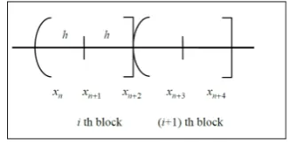
In order to evaluate the approximate solution in each block, the interval [a,b] is divided into
a series of blocks that each block contains k
points. The approximate solution at the point
xn is used to start thei thblock while the ap-proximate solution at the pointxn+kis the last point in the i th block. Then, the evaluation information at the last point in the i th block will be restored as the approximate solution at the point xn to start the (i+ 1) th block and the process continues for the next block.
Figure 1: 2-point block method.
A. Two - Point Second Derivative Implicit Block Method
In two point block method, the interval [a,b] contains two points for each block with the step size 2h (refer to Figure1). The two values of yn+1 and yn+2 are calculated concurrently
in a block. For the evaluation of yn+1 take
xn+1 = xn +h and integrating (1) over the interval [xn, xn+1] gives :
Z xn+1
xn
y0dx= Z xn+1
xn
f(x, y)dx,
y(xn+1) =y(xn) + Z xn+1
xn
f(x, y)dx. (3)
Then,f(x, y) in (3) will be replaced by Her-mite Interpolating Polynomial in (2) and define
p2(x) as follows,
p2(x) = [(
x−xn+1
xn−xn+1
)( x−xn+2
xn−xn+2
)2−(( 2
xn−xn+2
)
+( 1
xn−xn+1
))(x−xn)( x−xn+1
xn−xn+1
)( x−xn+2
xn−xn+2
)2]f0
+[( x−xn
xn+1−xn
)2( x−xn+2
xn−xn+2
)2]f1+[(
x−xn
xn+2−xn )2
( x−xn+1
xn+2−xn+1
)−(( 1
xn+2−xn+1
)+( 2
xn+2−xn ))
(x−xn+2)(
x−xn
xn+2−xn
)2( x−xn+1
xn+2−xn+1
)]f2
+[(x−xn)(
x−xn+1
xn−xn+1
)(x−xn+2
xn−xn+2
)2]g0
+[(x−xn+2)(
x−xn
xn+2−xn
)2( x−xn+1
xn+2−xn+1
)]g2.
(4)
Letx=xn+2+s hand
s= x−xn+2
h . (5)
Replacedx =h ds and change the limit of in-tegration from -2 to -1 in (3) we obtain:
y(xn+1) =y(xn) + Z −1
−2
[f0L0,0(s) +f1L1,0(s)
+f2L2,0(s) +g0L0,1(s) +g2L2,1(s)] h ds. (6)
where
L0,0(s) =−
1 4(s
3+s2)−1
2(s
3+ 2s2)(s+ 1),
L1,0(s) =s2(s+ 2)2,
L2,0(s) =
1
4(s+ 2)
2(s+ 1)−1
2(s
2+s)(s+ 2)2,
L1,0(s) =−
h
4 s
2 (s+ 2) (s+ 1),
L2,1(s) =
h
4 s(s+ 2)
2(s+ 1).
Evaluating the integral in (6) by using MAPLE produces the first formula of the two-point im-plicit block method as follows,
yn+1 =yn+
h
240[131fn+ 128fn+1−19fn+2]
+ h
2
240[23gn+ 7gn+2]. (7)
Now, integrating (1) over the interval [xn, xn+2] to obtain the approximate solutions
of yn+2 we have
Z xn+2
xn
y0dx= Z xn+2
xn
f(x, y)dx,
y(xn+2) =y(xn) + Z xn+2
xn
f(x, y)dx. (8)
Then,f(x, y) in (8) will be replaced by Her-mite Interpolating Polynomial in (4). Also, by replacing (5) letting dx = h ds and changing the limit of integration from -2 to 0 in (8) we obtain:
y(xn+2) =y(xn) +
Z 0
−2
+f2L2,0(s) +g0L0,1(s) +g2L2,1(s)]h ds. (9)
Evaluating the integral in (9) by using MAPLE produces the second formula of the two-point Implicit block method as follows,
yn+2 =yn+
h
15[7fn+ 16fn+1+ 7fn+2]
+h
2
15[gn−gn+2]. (10)
B. Three - Point Second Derivative Implicit Block Method
In the three points block, the interval [a,b] contains three points for each block with the step size 3h (refer to Figure 2). The three approximation values of yn+1, yn+2 and yn+3
at the point xn+1, xn+2 and xn+3 are
calcu-lated concurrently in a block. The derivations of the three point block method are similar to the previous derivations of the two point block method.
Equation (1) will be integrated over the in-terval [xn, xn+1], [xn, xn+2] and [xn, xn+3] to
obtian the approximate solutions ofyn+1,yn+2
and yn+3, definedp3(x) as follows,
p3(x) = [(
x−xn+1
xn−xn+1
)( x−xn+1
xn−xn+1
)( x−xn+3
xn−xn+3
)2
+(( −1
xn−xn+1
) + ( −1
xn−xn+2
) + ( −2
xn−xn+3
))
((x−xn)( x−xn+1
xn−xn+1
)( x−xn+2
xn−xn+2
)( x−xn+3
xn−xn+3
)2)]f0+
[( x−xn
xn+1−xn
)2( x−xn+2
xn+1−xn+2
)( x−xn+3
xn+1−xn+3
)2]f1
+[( x−xn
xn+2−xn
)2( x−xn+1
xn+2−xn+1
) ( x−xn+3
xn+2−xn+3
)2]f2
+[( x−xn
xn+3−xn
)2( x−xn+1
xn+3−xn+1
)( x−xn+2
xn+3−xn+2
)
−(( 2
xn+3−xn
)+( 1
xn+3−xn+1
)+( 1
xn+3−xn+2
))
((x−xn+3)(
x−xn
xn+3−xn
)2( x−xn+1
xn+3−xn+1
)
( x−xn+2
xn+3−xn+2
))]f3+ ((x−xn)(
x−xn+1
xn−xn+1
)
( x−xn+2
xn−xn+2
)( x−xn+3
xn−xn+3
)2)g0+ ((x−xn+3)
( x−xn
xn+3−xn
)2( x−xn+1
xn+3−xn+1
)( x−xn+2
xn+3−xn+2
))]g3.
(11)
Then, Hermite Interpolating Polynomial in (11) will interpolate f(x, y) and let
x = xn+3 +sh and s = x−xhn+3. For each
evaluation of yn+1, yn+2 and yn+3, we take
xn+1 = xn + h, xn+2 = xn+1 + h and
xn+3 =xn+2+h respectively.
The first , second and third point can be writ-ten as follows,
yn+1=yn+
h
6480[3463fn+ 3537fn+1−783fn+2
+263fn+3] +
h2
1080[97gn−17gn+3].
yn+2 =yn+
h
405[181fn+ 459fn+1+ 189fn+2
−19fn+3] +
h2
135[8gn+ 2gn+3].
yn+3=yn+
h
80[39fn+ 81fn+1+ 81fn+2
+39fn+3] +
h2
40[3gn−3gn+3]. (12)
III.
Order Conditions And
Error Constant Of The
New Methods
This section presents a definition of the order of the two and three point block methods that have been derived in this paper.
According to Fatunla (1991) and Lambert (1991), the local truncation error associated with normalized form of the new method can be defined as the linear difference operator
L[Z(x);h] = k X
i=0
αiZ(x+jh)− k X
i=0
−
k X
i=0
h2γiZ00(x+jh). (13)
Assuming that Z(x) is sufficiently differen-tiable, (13) can be expanded as a Taylor series expansion about the point x to obtain the ex-pressionL[Z(x);h] =C0Z(x)+C1hZ0(x)+...+
CphpZp(x) +...,where the constant coefficients
Cp, p= 0,1, ...are given as follows:
C0 =
k X
i=0
αj,
C1 =
k X
i=0
jαj− k X
i=0
βj,
Cp= 1
p! k X
i=0
jpαj− 1 (p−1)!
k X
i=0
jp−1βj
− 1
(p−2)! k X
i=0
jp−2γj, p= 2,3, .. (14)
According to Henrici (1962), it can be said that the new method has order p if
C0 =C1=...=Cp= 0, Cp+1 6= 0.
Therefore, Cp+1 is the error constant and
Cp+1hp+1Z(p+1)(xn) is the principal local
truncation error at the pointxn.
The formulae of a new two point block method is given by (7) and (10) and the formulae is written into a matrix as follows:
αYm = +hβFm+h2γGm (15)
whereα, β and γ are the coefficients with the m-vector Ym, Fm and Gm be defind as,
α=
−1 1 0
−1 0 1 , β= 131 240 128 240 −19 240 7 15 16 15 7 15 , γ = 23 240 0 7 240 1 15 0 −1 15 ,
Ym =
yn
yn+1
yn+2
, Fm =
fn
fn+1
fn+2
, Gm =
gn
gn+1
gn+2
.
α0 =
−1
−1
, α1=
1 0
, α2 =
0 1
,
β0=
131
240 7 15
, β1=
128
240 16 15
, β2=
−19 240 7 15 ,
γ0 =
23
240 1 15
, γ1 =
0 0
, γ2 =
7 240 −1 15 .
Forp= 0,
C0= 2
X
i=0
αj =
0 0
,
Forp= 1,
C1= 2
X
i=0
jαj−
2
X
i=0
βj =
0 0
,
Forp= 2,
C2 =
1 2!
2
X
i=0
j2αj−
2
X
i=0
jβj−
2
X
i=0
γj =
0 0
,
Forp= 3,
C3=
1 3!
2
X
i=0
j3αj− 1 (2)!
2
X
i=0
j2βj
−
2
X
i=0
jγj =
0 0
,
Forp= 4,
C4 =
1 4!
2
X
i=0
j4αj− 1 (3)!
2
X
i=0
j3βj−
1 (2)!
2
X
i=0
j2γj =
0 0
,
Forp= 5,
C5=
1 5!
2
X
i=0
j5αj− 1 (4)!
2
X
i=0
− 1
(3)!
2
X
i=0
j3γj =
0 0
,
For p= 6,
C6 =
1 6!
2
X
i=0
j6αj− 1 (5)!
2
X
i=0
j5βj
− 1
(4)!
2
X
i=0
j4γj = −1 720 0 6 = 0 0 .
Then, the 2-point implicit block method has order p= 5 and error constant C6 = [720−1,0]T.
The formulae of a new three point block method is given by (12) and the formulae is written into a matrix from (15) as follows:
α=
−1 1 0 0
−1 0 1 0
−1 0 0 1
, β = 3463 6480 3537 6480 −783 6480 263 6480 181 405 459 405 189 405 −19 405 39 80 81 80 81 80 39 80 , γ = 97
1080 0 0 −17 1080 8
135 0 0 2 135 3
40 0 0 −3
40
,
Ym=
yn
yn+1
yn+2
yn+3
, Fm=
fn
fn+1
fn+2
fn+3
, Gm=
gn
gn+1
gn+2
gn+3
.
α0=
−1 −1 −1
, α1=
1 0 0
, α2 =
0 1 0
, α3 =
0 0 1 ,
β0=
3463 6480 181 405 39 80
, β1=
3537 6480 459 405 81 80
, β2=
−783 6480 189 405 81 80 ,
β3=
263 6480 −19 405 39 80
, γ0=
97 1080 8 135 3 40
, γ1=
0 0 0 ,
γ2=
0 0 0
and γ3 = −17 1080 2 135 −3 40 .
For p= 0,
C0 = 3
X
i=0
αj = 0 0 0 ,
Forp= 1,
C1 = 3
X
i=0
jαj−
3
X
i=0
βj = 0 0 0 ,
Forp= 2,
C2 =
1 2!
3
X
i=0
j2αj −
3
X
i=0
jβj −
3
X
i=0
γj = 0 0 0 ,
Forp= 3,
C3=
1 3!
3
X
i=0
j3αj− 1 (2)!
3
X
i=0
j2βj−
3
X
i=0
jγj = 0 0 0 ,
Forp= 4,
C4 =
1 4!
3
X
i=0
j4αj− 1 (3)!
3
X
i=0
j3βj−
1 (2)!
3
X
i=0
j2γj = 0 0 0 ,
Forp= 5,
C5=
1 5!
3
X
i=0
j5αj− 1 (4)!
3
X
i=0
j4βj
− 1
(3)!
3
X
i=0
j3γj = 0 0 0 ,
Forp= 6,
C6=
1 6!
3
X
i=0
j6αj− 1 (5)!
3
X
i=0
− 1
(4)!
3
X
i=0
j4γj = 0 0 0 ,
For p= 7,
C7 =
1 7!
3
X
i=0
j7αj− 1 (6)!
3
X
i=0
j6βj
− 1
(5)!
3
X
i=0
j5γj = 97 100800 −1 6300 9 11200
6= 0 0 0 .
Then, the 3-point implicit block method has order p = 6 and error constant
C7 = [10080097 ,6300−1 ,112009 ]T.
IV.
The Zero-Stability Of
The Methods
In this section, the zero-stability of the 2-point and 3-point implicit block method are dis-cussed.
Two point implicit block method
The general form of (7) and (10) can be writ-ten in the matrix form :
1 0 0 1
yn+1
yn+2
=
0 1 0 1
yn−1
yn +h 131 240 128 240 −19 240 7 15 16 15 7 15 fn
fn+1
fn+2
+h2
23 240 0 7 240 1 15 0 −1 15 gn
gn+1
gn+2
.
The first characteristic polynomial of the 2-point implicit block method is given as follows,
ρ(R) = det [RA(0)−A(1)] = 0, where
A(0)=
1 0 0 1
and A(1)=
0 1 0 1
.
ρ(R) = det
R −1 0 R−1
= 0, R(R−1) =
0, R= 0,1,|R|≤1.
Three point implicit block method
The general form of (12) can be written in the matrix form :
1 0 0 0 1 0 0 0 1
yn+1
yn+2
yn+3
=
0 0 1 0 0 1 0 0 1
yn−2
yn−1
yn +h 3463 6480 3537 6480 −783 6480 263 6480 181 405 459 405 189 405 −19 405 39 80 81 80 81 80 39 80 fn
fn+1
fn+2
fn+3
+h2
97
1080 0 0 −17 1080 8
135 0 0 2 135 3
40 0 0 −3 40 gn
gn+1
gn+2
gn+3
.
The first characteristic polynomial of the 3-point implicit block method is given as follows,
ρ(R) = det [RA(0)−A(1)] = 0, where
A(0) =
1 0 0 0 1 0 0 0 1
and A(1) =
0 0 1 0 0 1 0 0 1
.
ρ(R) = det
R 0 −1 0 R −1 0 0 R−1
=
0, R2(R−1) = 0, R= 0,0,1 ,|R|≤1.
V.
Implementation
This section focuses on the explanation of the implementation of the two and three point implicit second derivative block methods.
Two point implicit second derivative block method
The values of yn+1 and yn+2 in (7) and (10)
will be approximated by using the predictor-corrector equations.
The predictor equations:
ynp+m=ycn+m h fnc, m= 1,2, (16)
fnp+m =f(xn+m, ynp+m),
gnp+m=f0(xn+m, ynp+m).
The corrector equations:
ycn+1=ync + h 240[131f
c
n+ 128f p
n+1−19f
p n+2]
+h
2
240[23g c n+ 7g
p n+2].
ync+2 =ycn+ h 15[7f
c n+ 16f
p
n+1+ 7f
p n+2]
+h
2
15[g c n−g
p n+2].
And the next corrector equations will be taken as follows:
ycn+1=ync + h 240[131f
c
n+ 128fnc+1−19fnc+2]
+h
2
240[23g c
n+ 7gcn+2].
ync+2 =ycn+ h 15[7f
c
n+ 16fnc+1+ 7fnc+2]
+h
2
15[g c
n−gnc+2].
fnc+m =f(xn+m, ync+m),
gnc+m=f0(xn+m, ync+m), m= 1,2.
Three point implicit second derivative block method
The values of yn+1, yn+2 and yn+3 in (12)
will be approximated by using the predictor-corrector equations.
The predictor equations:
Define (16) as the predictor equations and let
m= 1,2,3.
The corrector equations:
ync+1=ync+ h
6480[3463f c
n+3537f p
n+1−783f
p n+2+
263fnp+3] + h
2
1080[97g c n−17g
p n+3].
ync+2=ync+ h 405[181f
c n+459f
p
n+1+189f
p
n+2−19f
p n+3]
+ h
2
135[8g c n+ 2g
p n+3].
ync+3=ync+h 80[39f
c n+81f
p
n+1+81f
p
n+2+39f
p n+3]
+h
2
40[3g c
n−3gnc+3].
And the next corrector equations will be taken as follows:
ync+1=ync+ h
6480[3463f c
n+3537fnc+1−783fnc+2+263fnc+3]
+ h
2
1080[97g c
n−17gcn+3].
ync+2=ync+ h 405[181f
c
n+459fnc+1+189fnc+2−19fnc+3]
+ h
2
135[8g c
n+ 2gnc+3].
ync+3=ync+h 80[39f
c
n+81fnc+1+81fnc+2+39fnc+3]
+h
2
40[3g c
n−3gnc+3].
fnc+m=f(xn+m, ycn+m),
VI.
Numerical Experiments
In this section, based on the new methods we developed C codes for solving first - order ordinary differential equation problems and compared the numerical results when the same set of problems are solved by using the existing methods .
Problem 1:
y0 =y−x2+ 1, y(0) = 1
2, [0,5].
Exact solution:y(x) = (1 +x)2−1
2e x.
Source Yaacob and Sanugi (1995).
Problem 2:
y0 =xy3−y, y(0) = 1, [0,10].
Exact solution:y(x) = √ 2
2 + 4x+ 2e2x. Source: Famurewa et al. (2011).
Problem 3:
y10 =y3, y1(0) = 1, [0, π].
y20 =y4, y2(0) = 1,
y30 =−e−xy2, y3(0) = 0,
y40 = 2exy3, y4(0) = 1.
Exact solution:y1(x) =cos(x),
y2(x) =excos(x),
y3(x) =−sin(x),
y4(x) =excos(x)−exsin(x).
Source : Abdul Majid et al. (2012).
Problem 4:
yi0 =−βiyi+yi2, i= 1,2,3,4, yi(0) =−1, [0,20].
with β1 = 0.2, β2= 0.2, β3= 0.3, β4 = 0.4.
Exact solution:yi(x) = βi 1 +cieβix
,
ci =−(1 +βi).
Source : Johnson and Barney (1976).
Notations used are as follows.
• h: step size.
• Time: seconds.
• Max Error: maximum error|y(xi)−yi|.
• New 2P: The new 2-point implicit second derivative block method derived in this pa-per.
• New 3P: The new 3-point implicit second derivative block method derived in this pa-per.
• method 2A: 2-point Implicit third deriva-tive block method proposed by Akinfenwa et al. (2015).
• method 3A: 3-point Implicit third deriva-tive block method proposed by Akinfenwa et al. (2015).
• method 2M : 2-point implicit block one-step method half Gauss-Seidel proposed by Majid et al. (2003).
• method S : A simpson’s-type second derivative block method proposed by Sahi et al. (2012).
Table 1: Numerical Results of the New 2P, 2A and Majid Methods for solving Problem 1.
h Methods MAXE Time New 2P 3.097580(-7) 0.008 0.1 2A 9.075473(-6) 0.009 Majid 1.028331(-3) 0.007
New 2P 3.096409(-9) 0.027 0.05 2A 2.336125(-7) 0.033 Majid 4.335581(-5) 0.026
New 2P 4.814321(-11) 0.072 0.025 2A 6.980545(-9) 0.074 Majid 2.708640(-6) 0.070
Table 2: Numerical Results of the New 2P, 2A and Majid Methods for solving Problem 2.
h Methods MAXE Time New 2P 8.068236(-7) 0.036 0.1 2A 2.407103(-5) 0.038 Majid 5.322828(-5) 0.035
New 2P 1.852646(-8) 0.079 0.05 2A 6.901808(-6) 0.081 Majid 4.287203(-6) 0.078
New 2P 3.577403(-10) 0.130 0.025 2A 1.925143(-6) 0.132 Majid 3.081526(-7) 0.128
New 2P 6.248941(-12) 0.155 0.0125 2A 5.110584(-7) 0.158 Majid 2.073222(-8) 0.154
Table 3: Numerical Results of the New 2P, 2A and Majid Methods for solving Problem 3.
h Methods MAXE Time New 2P 4.803249(-6) 0.046 0.1 2A 6.021320(-6) 0.047 Majid 7.434949(-5) 0.045
New 2P 1.380934(-7) 0.094 0.05 2A 9.966465(-7) 0.096 Majid 4.751417(6) 0.093
New 2P 4.138981(-9) 0.141 0.025 2A 8.262003(-8) 0.143 Majid 3.003513(-7) 0.140
New 2P 1.266727(-10) 0.175 0.0125 2A 5.800818(-9) 0.177 Majid 1.887970(-8) 0.174
Table 4: Numerical Results of the New 2P, 2A and Majid Methods for solving Problem 4.
h Methods MAXE Time New 2P 1.085710(-5) 0.062 0.1 2A 3.864142(-4) 0.063 Majid 4.230879(-4) 0.060
New 2P 7.773816(-7) 0.171 0.05 2A 3.396333(-5) 0.173 Majid 3.499478(-5) 0.169
New 2P 3.393665(-8) 0.296 0.025 2A 3.873437(-6) 0.298 Majid 2.530419(-6) 0.294
New 2P 1.239543(-9) 0.483 0.0125 2A 4.865963(-7) 0.485 Majid 1.703761(-7) 0.481
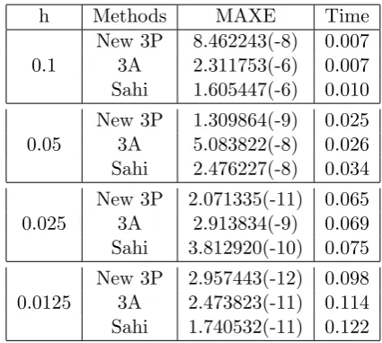
Table 5: Numerical Results of the New 3P, 3A and Sahi Methods for solving Problem 1.
h Methods MAXE Time New 3P 8.462243(-8) 0.007 0.1 3A 2.311753(-6) 0.007 Sahi 1.605447(-6) 0.010
New 3P 1.309864(-9) 0.025 0.05 3A 5.083822(-8) 0.026 Sahi 2.476227(-8) 0.034
New 3P 2.071335(-11) 0.065 0.025 3A 2.913834(-9) 0.069 Sahi 3.812920(-10) 0.075
Table 6: Numerical Results of the New 3P, 3A and Sahi Methods for solving Problem 2.
h Methods MAXE Time New 3P 1.368469(-7) 0.032 0.1 3A 1.897087(-5) 0.034 Sahi 1.350523(-7) 0.036
New 3P 5.097240(-9) 0.072 0.05 3A 6.888210(-6) 0.074 Sahi 9.439226(-9) 0.080
New 3P 8.308907(-11) 0.126 0.025 3A 2.049793(-6) 0.127 Sahi 6.071470(-10) 0.131
New 3P 1.311735(-12) 0.151 0.0125 3A 5.595309(-7) 0.153 Sahi 3.812597(-11) 0.157
Table 7: Numerical Results of the New 3P, 3A and Sahi Methods for solving Problem 3.
h Methods MAXE Time New 3P 2.941061(-6) 0.040 0.1 3A 4.800874(-5) 0.041 Sahi 7.541150(-5) 0.046
New 3P 8.019770(-8) 0.089 0.05 3A 6.981759(-7) 0.091 Sahi 3.244254(-6) 0.095
New 3P 2.349645(-9) 0.136 0.025 3A 1.057838(-8) 0.137 Sahi 1.087780(-7) 0.141
New 3P 7.114069(-11) 0.172 0.0125 3A 1.630123(-10) 0.174 Sahi 3.662937(-9) 0.175
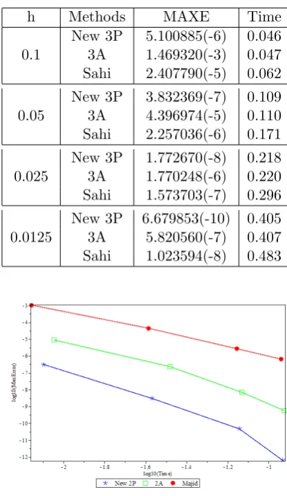
Table 8: Numerical Results of the New 3P, 3A and Sahi Methods for solving Problem 4.
h Methods MAXE Time New 3P 5.100885(-6) 0.046 0.1 3A 1.469320(-3) 0.047 Sahi 2.407790(-5) 0.062
New 3P 3.832369(-7) 0.109 0.05 3A 4.396974(-5) 0.110 Sahi 2.257036(-6) 0.171
New 3P 1.772670(-8) 0.218 0.025 3A 1.770248(-6) 0.220 Sahi 1.573703(-7) 0.296
New 3P 6.679853(-10) 0.405 0.0125 3A 5.820560(-7) 0.407 Sahi 1.023594(-8) 0.483
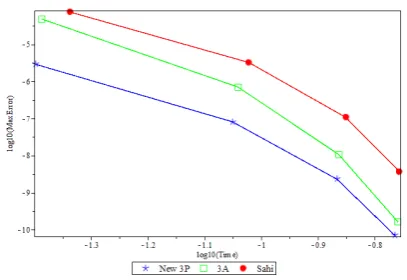
Figure 4: The Efficiency curves for Problem 2 (2-point block method) with step size h = 0.1,0.05,0.025,0.0125.
Figure 5: The Efficiency curves for Problem 3 (2-point block method) with step size h = 0.1,0.05,0.025,0.0125.
Figure 6: The Efficiency curves for Problem 4 (2-point block method) with step size h = 0.1,0.05,0.025,0.0125.
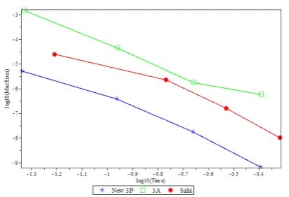
Figure 7: The Efficiency curves for Problem 1 (3-point block method) with step size h = 0.1,0.05,0.025,0.0125.
Figure 8: The Efficiency curves for Problem 2 (3-point block method) with step size h = 0.1,0.05,0.025,0.0125.
Figure 10: The Efficiency curves for Problem 4 (3-point block method) with step size h = 0.1,0.05,0.025,0.0125.
VII.
Results and Discussion
In this paper, we presented the derivation of two and three point second derivatives implicit block methods for solving first-order ODEs. The numerical results are tabulated in Tables 1-8 and are plotted in Figures 3-10. Those figures showed the efficiency curves, where the common logarithm of the maximum global errors were plotted versus the computational time. Figures 3-6 revealed that 2P (2- point order 5 second derivative block method derived in this paper) is the most efficient compared to 2A (2-point one-step order 5 implicit third derivative block multistep method) and Majid (2-point implicit block method). Tables 1-4 showed that the new 2P method has less maximum error compared with 2A and Majid methods. Figures 7-10 showed that the new 3P (3- point order 6 second derivative block method derived in this paper) is the most effi-cient compared to 3A (order 6, 3-point implicit third derivative block multistep method) and Sahi (Simpson’s type order 6 second derivative block method). Tables 5-8 showed that the new 3P method has less maximum error and less computational time compared to 3A and Sahi’s methods.
Numerical results revealed that the new 2P and 3P methods are more efficient as
compared to the existing methods and they also illustrated that the new second deriva-tive block methods are more accurate and competent for solving first order ODEs.
References
[1] Zanariah Abdul Majid, Nur Zahidah Mokhtar, and Mohamed Suleiman. Di-rect two-point block one-step method for solving general second-order ordinary dif-ferential equations. Mathematical
Prob-lems in Engineering, 2012, 2012.
[2] OA Akinfenwa, B Akinnukawe, and SB Mudasiru. A family of continu-ous third derivative block methods for solving stiff systems of first order ordi-nary differential equations. Journal of
the Nigerian Mathematical Society, 34
(2):160–168, 2015.
[3] OK Famurewa, RA Ademiluyi, and DO Awoyemi. A comparative study of a class of implicit multi-derivative meth-ods for numerical solution of non-stiff and stiff first order ordinary differential equations. African Journal of
Mathemat-ics and Computer Science Research, 4(3):
120–135, 2011.
[4] Simeon Fatunla. Block methods for sec-ond order odes. International journal
of computer mathematics, 41(1-2):55–63,
1991.
[5] Peter Henrici. Discrete variable methods
in ordinary differential equations. John
Wiley & Sons, Inc., 1962.
[6] Zarina Bibi Ibrahim, Khairil Iskandar Othman, and Mohamed Suleiman. Im-plicit r-point block backward differenti-ation formula for solving first-order stiff odes. Applied Mathematics and
[7] Zarina Bibi Ibrahim, Mohamed Suleiman, and Khairil Iskandar Oth-man. Fixed coefficients block backward differentiation formulas for the numeri-cal solution of stiff ordinary differential equations. European Journal of Scientific
Research, 21(3):508–520, 2008.
[8] Zarina Bibi Ibrahim, Mohamed Suleiman, NAAM Nasir, and Khairil Iskandar Othman. Conver-gence of the 2-point block backward differentiation formulas. Applied
Math-ematical Sciences, 5(70):3473–3480,
2011.
[9] AI Johnson and JR Barney. Numeri-cal solution of large systems of stiff ordi-nary differential equations.Modular Sim-ulation Framework, Numerical Methods for Differential Systems, Academic Press
Inc., New York, pages 97–124, 1976.
[10] GM Kumleng and UWW Sirisena. A (α)-stable order ten second derivative block multistep method for stiff initial value problems. International Journal of Mathematics and Statistics Invention
(IJMSI), 2(10):37–43, 2014.
[11] John Denholm Lambert. Numerical methods for ordinary differential systems:
the initial value problem. John Wiley &
Sons, Inc., 1991.
[12] Zanariah Abdul Majid, Mohamed Suleiman, Fudziah Ismail, and Mohamed Othman. 2-point implicit block one-step method half gauss-seidel for solving first order ordinary differential equations.
Matematika, 19:91–100, 2003.
[13] Zanariah Abdul Majid, Mohamed Bin Suleiman, and Zurni Omar. 3-point implicit block method for solving ordi-nary differential equations. Bulletin of the Malaysian Mathematical Sciences
Society. Second Series, 29(1):23–31,
2006.
[14] S Mehrkanoon, ZA Majid, M Suleiman, KI Othman, and ZB Ibrahim. 3-point implicit block multistep method for the solution of first order odes. Bulletin of the Malaysian Mathematical Sciences
So-ciety, 35(2A), 2012.
[15] RK Sahi, SN Jator, and NA Khan. A simpson’s-type second derivative method for stiff systems. International journal
of pure and applied mathematics, 81(4):
619–633, 2012.
[16] Nazeeruddin Yaacob and Bahrom Sanugi. A New 3-stage Fourth Order,
RK-NHM34 Method for Solving Y.