Comparative Analysis of Mice Protein Expression: Clustering and Classification Approach

© Penerbit UTHM DOI: https://doi.org/10.30880/ijie.2018.10.06.004

Comparative Analysis of Mice Protein Expression: Clustering

and Classification Approach

Mohd Zainuri Saringat

, Aida Mustapha

, Rachmadita Andeswari

1

Faculty of Computer Science and Information Technology, Universiti Tun Hussein Onn Malaysia, 86400, Johor, Malaysia

2

School of Computing, Telkom University, 40257 Bandung, West Java, Indonesia Received 28 June 2018; accepted 5 August 2018, available online 24 August 2018

1. Introduction

Down Syndrome (DS) is a genetic disorder causing a lifelong condition that is associated with cognitive disability and physical abnormalities due to a defect involving chromosome 21, which is the existence of an extra copy of the trisomy-21 chromosome. This chromosomal anomaly was discovered by a French physician Jerome Lejeune in 1959 when he observed 47 in the cells of individuals with Down syndrome [1]. This disease is known to affect one in 1000 live born human.

For preclinical evaluation of drug effects in diagnosing DS, [2] created a protein expression dataset for 38 control mice and 34 trisomic mice (mice with DS). This dataset categorized the mice based on features such as their genotype, behavioral and drug treatment called memantine. Some mice were stimulated to learn context-shock while others were not. Some were injected with memantine while others were not.

This research attempts to analyze protein influences that could have affected the recovering ability to learn among the trisomic mice by performing a comparative analysis on two data mining approaches, which are clustering and classification. The remainder of this paper is structured as follows. Section 2 presents the domain in brief, Section 3 presents the methodology used for the proposed analysis, Section 4 presents the results.Finally Section 5 concludes the papers.

2. Related Work

Medical data mining has employed various data mining tasks such as classification and clustering to assist medical diagnosis using general medical datasets [3] or specific disease such as the Wisconsin Diagnostic Breast Cancer (WDBC) dataset [4] and the Tumor Rnaseq Expression dataset [5]. Both supervised and unsupervised learning have been shown to be very useful in analysis of such datasets.

Research using the Mice Protein Expression dataset was initiated by [2]. Subsequent research such as [6] revealed that nine proteins have been chosen as strong candidates for future biomarkers. Meanwhile, K-NN and Neural Network had the better overall performances and highest accuracies (86.26% ± 0.23%; 81.51% ± 0.48%), which makes them a promising predictive tool to study protein profiles in DS patients’ follow-up after treatment with memantine. Research by [7] succeeded with 94.35% accuracy using Bayesian Network, 99.26% accuracy using KNN, 95.46% accuracy using Decision Table, 100% accuracy with Random Forest and 100% accuracy with SVM.

Feature Maps (SOM), Growing Cell Structures (GCS), K-means, and hierarchical clustering.

In contrast to unsupervised learning is the supervised learning, which is used when data instances belong to a set of pre-determined classes or class labels. Supervised learning methods include rule-based classifiers, Support Vector Machine (SVM), decision trees, and Bayesian classifiers. Their goal is to build a general model that can subsequently be used to classify new, unlabeled (or simply called the testing) data instances.

3.

Methodology

This paper presents a comparative analysis of the mice protein expression using two different data mining approaches; clustering and classification. A standard data mining processes based on the Knowledge Discovery in Databases (KDD) framework [9]. KDD refers to the overall process of discovering useful knowledge from the data by evaluating and interpreting patterns in order to make decisions of what qualifies as knowledge. The framework is shown in Fig. 1.

Based on Fig. 1, there are five phases in the KDD including the selection of encoding schemes, data pre-processing, sampling, and transformation before the data is ready for mining.

Fig. 1 Standard KDD framework [9].

The fourth step in KDD framework is data mining. There are four major data mining tasks, which are classification or prediction, clustering, association rule mining, and anomaly detection. In this paper, the data mining framework used is the combination of clustering and classification as shown in Fig. 2.

Fig. 2 Comparative analysis framework for protein mice expression

The comparative analysis performed based on the proposed framework in Fig. 2 will be applied onto the Mice Protein Expression dataset in effort to analyze the protein influences that could have affected the recovering ability to learn among the trisomic mice.

3.1 Dataset

In this project, the Mice Protein Expression dataset was sourced from the UCI machine learning database [2]. The dataset consists of the expression levels of 77 protein modifications that produced detectable signals in the nuclear fraction of cortex. There were 38 control mice and trisomic mice, for a total of 72 mice (7-10 mice in each of the eight groups). According to [2], the dataset contains one or more missing mice protein values and were replaced with the average value of expression level in the same class of mice during the pre-processing phase. The work also indicated that one variable, which is the t-CS-m (trisomic-context shock-memantine), had missing values for the majority of proteins and therefore was excluded from the dataset.

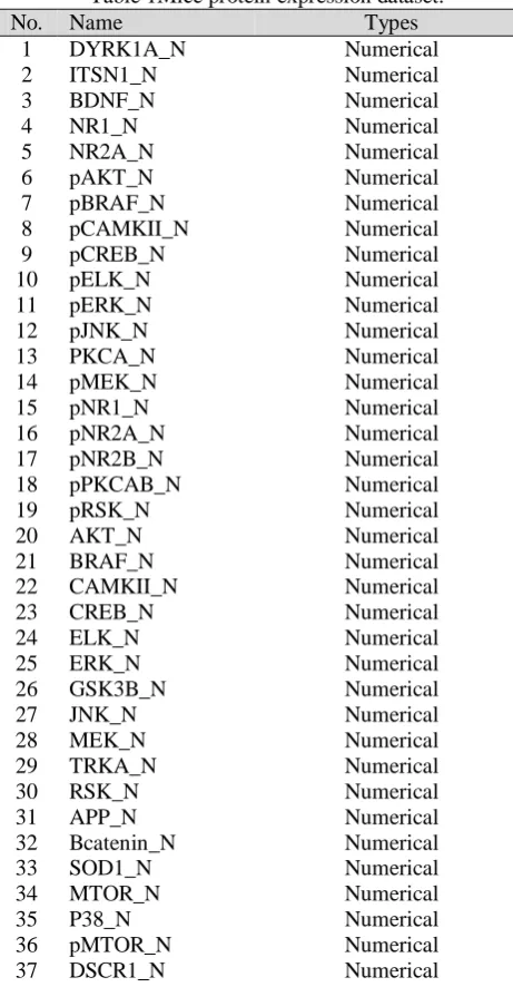
Table 1 shows the list of features and type of each feature used in the experiment. As shown, the protein expression data were generated from additional subcellular fractions from both cortex and hippocampus of the same mice. However, the cortex nuclear fraction was chosen for use here because it was the most complete of the datasets.

Table 1Mice protein expression dataset.

No. Name Types

1 DYRK1A_N Numerical

2 ITSN1_N Numerical

3 BDNF_N Numerical

4 NR1_N Numerical

5 NR2A_N Numerical

6 pAKT_N Numerical

7 pBRAF_N Numerical

8 pCAMKII_N Numerical

9 pCREB_N Numerical

10 pELK_N Numerical

11 pERK_N Numerical

12 pJNK_N Numerical

13 PKCA_N Numerical

14 pMEK_N Numerical

15 pNR1_N Numerical

16 pNR2A_N Numerical

17 pNR2B_N Numerical

18 pPKCAB_N Numerical

19 pRSK_N Numerical

20 AKT_N Numerical

21 BRAF_N Numerical

22 CAMKII_N Numerical

23 CREB_N Numerical

24 ELK_N Numerical

25 ERK_N Numerical

26 GSK3B_N Numerical

27 JNK_N Numerical

28 MEK_N Numerical

29 TRKA_N Numerical

30 RSK_N Numerical

31 APP_N Numerical

32 Bcatenin_N Numerical

33 SOD1_N Numerical

34 MTOR_N Numerical

35 P38_N Numerical

36 pMTOR_N Numerical

38 AMPKA_N Numerical

39 NR2B_N Numerical

40 pNUMB_N Numerical

41 RAPTOR_N Numerical

42 TIAM1_N Numerical

43 pP70S6_N Numerical

No. Name Types

44 NUMB_N Numerical

45 P70S6_N Numerical

46 pGSK3B_N Numerical

47 pPKCG_N Numerical

48 CDK5_N Numerical

49 S6_N Numerical

50 ADARB1_N Numerical

51 AcetylH3K9_N Numerical

52 RRP1_N Numerical

53 BAX_N Numerical

54 ARC_N Numerical

55 ERBB4_N Numerical

56 nNOS_N Numerical

57 Tau_N Numerical

58 GFAP_N Numerical

59 GluR3_N Numerical

60 GluR4_N Numerical

61 IL1B_N Numerical

62 P3525_N Numerical

63 pCASP9_N Numerical

64 PSD95_N Numerical

65 SNCA_N Numerical

66 Ubiquitin_N Numerical

67 pGSK3B_Tyr216_N Numerical

68 CaNA_N Numerical

69 Genotype Nominal

70 Treatment Nominal

71 Behavior Nominal

3.2 Clustering Algorithms

The clustering algorithms employed in the experiments include the K-Means, Hierarchal Clustering and Decision Tree.

• K-Means – K-Means clustering is a method of cluster analysis which aims to partition observation into k clusters in which each observation belongs to the cluster with the nearest mean [10]. It is an exclusive clustering algorithm that means each object is assigned to precisely one of a set of clusters. Objects in one cluster are similar to each other. The similarity between objects is based on a measure of the distance between them.

• Hierarchical Clustering – Hierarchical clustering algorithm is a commonly used text clustering method, which can generate hierarchical nested classes. It clusters similar instances in a group by using similarities of them. This requires the use of a similarity (distance) measure (usually the distance Euclidean) and cosine similarity for documents. Therefore, a similarity (distance) matrix of instances has to be created before running the method.

• Decision Tree – Decision tree is one of the most frequently used clustering model in data mining.

A decision tree is composed of root, branches and leaves. A tree structure develops from root and leaves and the most outer part is the root joint. Each inner joint of tree is separated to make the best decision with help of algorithms [11].

3.3 Classification Algorithm

The classification experiment in this project uses three classification algorithms from [12], which are the k -Nearest Neighbor, Random Forest, and Naïve Bayes.

• k-Nearest Neighbor – k-Nearest Neighbor is a type of lazy learning approach, whereby it learns by comparing a given test tuple with training tuples and classify into a particular tuple it is most similar with. For k-Nearest Neighbor classification, the unknown is assigned the most common class among its k neighbors. When k is 1, the unknown tuple is assigned the class of the training tuple that is closest to it in pattern space. Each tuple is represented by n attributes and a class, therefore the similarity is determined by the distance between the attributes within the tuples.

• Random Forest – Random Forest is an ensemble of many decision tree classifiers that in principal grow the trees into a forest. The random forest is generated based on randomly selected singular decisions trees at each node to determine the split. Each tree depends on the values of a random vector sampled independently and with the same distribution for all trees in the forest.

• Naïve Bayes – Naïve Bayes belongs to Bayesian classifier, which is a type of statistical classifier with a strong assumption that one variable is independent from another. This means when Naïve Bayes predicts the probability that a given tuple belongs to a particular class, it does not take into account the probable relationships between the variables within the tuples. Naïve Bayes classifiers originate from Bayes’ Theorem. Naïve Bayes applies the Bayes’ Theorem, whereby the class membership of an instance, x, is determined according to the class that has the highest posterior probability, conditioned on x [13].

4.

Results and Discussion

The results are presented in two sections based on the experimental setup, which is clustering and classification using the RapidMiner [14] and WEKA [15.

4.1 Clustering Experiment

The K-Means operator is applied on this dataset with default values for all parameters. As parameter k was set to 2, only two clusters are possible. That is why each example is assigned to either “cluster_0” or “cluster_1” as shown in Fig. 3.

stimulus and will freeze upon re-exposure to the same cage.

• Cluster_1 – This set of mice has normal genotype, treatment by memantine and has shock-context which us the mice that not learn to associate the novel cage with the shock and do not freeze upon re-exposure to the same cage.

Fig.3Generated k-means clusters.

For clustering, the agglomerative (bottom-up) hierarchical clustering has been used. An agglomerative clustering algorithm starts with clusters which each of them contain only one instance and for each iteration merges the most similar clusters until the stopping criterion is met such as a requested number k of clusters is achieved. The algorithms for agglomerative clustering is as follows:

1.

Start by assigning each item to its own

cluster, so that if there are

N

items, there

will be

N

clusters, each containing just

one item. Let the similarities between

the clusters equal to the similarities

between the items they contain.

2.

Find the most similar pair of clusters

and merge them into a single cluster, so

that now there will be one cluster lesser.

3.

Compute similarities between the new

cluster and each of the old clusters.

4.

Repeat steps 2 and 3 until all items are

clustered into a single cluster of size

N

.

At the third step, the similarity (or distance) matrix is updated after merging two clusters using single-link method. In this method, the linkage function or the distance D(X,Y) between clusters X and Yis described by the following equation:

𝐷𝐷(𝑋𝑋, 𝑌𝑌) = max_{𝑥𝑥∈𝑋𝑋,𝑦𝑦∈𝑌𝑌}𝑑𝑑(𝑥𝑥, 𝑦𝑦)

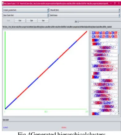
Fig. 4 shows the generated hierarchical clusters based on the mice protein expression dataset.Based on Fig. 4, the output shows that each cluster comes together. The value “1” represents that everything in that cluster shares the same value of one, and a value “0” represents that everything in that cluster has a value of zero for that attribute. Numbers are the average value of everyone in the cluster. From the total of 1080 instances with 71 features, each cluster shows the following types of behavior:

• Cluster_0 (c-CS-m) = 525 instances = 48.6%

• Cluster_1 (c-SC-m) = 555 instances = 51.4%

Finally, the decision tree was used to cluster protein expression data from the eight classes of mice. For both control and Ts65Dn, two groups of mice were trained in CS, injected with either saline or memantine and two groups were not trained in CF`C, also injected either with saline or memantine. The Ts65Dn CS mice injected with saline fail to learn the CFC task, but if injected with memantine, they learn successfully, while control CS mice learn equally well with either saline or memantine.

Fig.4Generated hierarchicalclusters.

Fig. 5 shows the sample generated tree from the protein mice expression dataset.

Fig. 5 Sample generated tree.

4.2 Classification Experiment

The classification experiment employed the hold-out validation method, whereby 60% of the 507 instances formed the training set and the remaining 40% formed the testing set. Table 2 shows the split on instances between the training and the testing set from the total of data samples.

Table 2Split between training and testing set of mice protein expression dataset.

Class Training Set Testing Set Total

t-CS-s 81 54 135

t-SC-s 63 42 105

t-SC-m 79 53 132

For the classification experiment, the main measure is the accuracy, precision, and recall across all three classification algorithms; k-Nearest Neighbor, Random Forest, and Naïve Bayes. The accuracy of classifier on a given test set is the percentage of test set tuples that correctly classified by the classifiers. Table 3 shows the classification results, which showed that the Random Forest algorithm achieved the highest accuracy percentage of 99.50% based on the 71 attributes with 0.995 of precision and recall.

Table 3Classification results for mice protein expression dataset.

Classifier k-NN Random _Forest Naïve _Bayes

Accuracy (%) 99.01 99.50 99.01

Precision 0.933 0.995 0.990

Recall 0.933 0.995 0.990

Meanwhile, k-Nearest Neighbor and Naïve Bayes classifier achieved the same accuracy of 99.01% but Naïve Bayes classifier achieved better precision and recall of 0.990 as compared to the k-NN classifier with only 0.933 rate of precision and recall.

5.

Conclusions

This paper used the mice protein expression data to perform clustering and classification analysis in determining protein in mouse model of down syndrome. Based on the clustering experiment, the clusters produced have been proven useful to identify common critical protein responses, which in turn helping in identifying potentially more effective drug targets. Meanwhile, all classification models implemented and compared in the classification experiments have efficiently classifies protein samples into the given eight classes with very high accuracy.

Acknowledgement

This project is sponsored by UniversitiTun Hussein Onn Malaysia.

References

[1] Wiseman F.K., Alford K.A., Tybulewics V.L.J., Fisher E.MC. Down syndrome-recent progress and future prospect, Hum Mol Genet. (2009), 18(R1):R75–83.

[2] Higuera, C., Gardiner, K. J.,Cios, K. J. Self-organizing feature maps identify proteins critical to learning in a mouse model of down syndrome. PloS one, (2015), 10(6), e0129126.

[3] Vanaja, S.,Rameshkumar, K. Performance Analysis of Classification Algorithms on Medical Diagnosis – A Survey. Journal of Computer Science, (2015), pp. 30-52.

[4] Alickovic, E.,Subasi, A. Data Mining Techniques for Medical Data Classification.(2011).

[5] Jagga, Z.,Gupta, D. Classification Models For Clear Cell Renal Carcinoma Stage Progression, Based on Tumor Rnaseq Expression Trained Supervised Machine Learning.(2014).

[6] Ribeiro-Machado, Cláudia, Sara Costa Silva, Sara Aguiar, and BrígidaMónicaFaria. Protein Attributes-Based Predictive Tool in a Down Syndrome Mouse Model: A Machine Learning Approach. In World Conference on Information Systems and Technologies, pp. 19-28. Springer, Cham, (2018).

[7] Furat, FahriyeGemci, and TurgayIbrikci. Classification of Down Syndrome of Mice Protein Dataset on MongoDB Database. Balkan Journal of Electrical and Computer Engineering 6, no. 2: 44-49 (2018).

[8] Hickendorff, M., Heiser, W.J., Putten, C.M.V. Verhelst,N.D. Clustering Nominal Data with Equivalent Categories. Behaviormetrika, (2008), 35(1): 35-54.

[9] Fayyad, U., Piatetsky-Shapiro, G.,Smyth, P. From data mining to knowledge discovery in databases. AI magazine, (1996), 17(3), 37.

[10] Berkhin, P. Survey of clustering data mining techniques, 2002. Accrue Software: San Jose, CA.(2004).

[11] Quinlan, J.R. C4.5 Programs for Machine Learning, Morgan Kaufmann, San Mateo, California.(1993). [12] Han, J., Pei, J.,Kamber, M. Data mining: concepts

and techniques. Elsevier.(2011).

[13] Samsudin, N. A.,Bradley, A. P. Extended Naive Bayes for Group Based Classification. In Proceeding of the First International Conference on Soft Computing and Data Mining (SCDM-2014), Springer, (2014), pp. 497-505.

[14] Hofmann, M., Klinkenberg, R. (Eds.). RapidMiner: Data mining use cases and business analytics applications. CRC Press. (2013).