BPGD-AG: A New Improvement
Of Back-Propagation Neural
Network Learning Algorithms
With Adaptive Gain
Nazri Mohd Nawi1, R.S. Ransing2, Norhamreeza Abdul Hamid1
1Faculty of Science Computer and Information Technology
Universiti Tun Hussein Onn Malaysia 86400, Parit Raja, Batu Pahat, Johor, MALAYSIA
2Civil and Computational Engineering Centre, School of Engineering
University of Wales Swansea
Singleton Park, Swansea, SA2 8PP, UNITED KINGDOM
Corresponding email : [email protected]
Abstract
1 INTRODUCTION
We consider standard multi-layer feed forward neural networks that have an input layer of neurons, a hidden layer of neurons and an output layer of neurons, and in that every node in a layer is connected to every other node in the adjacent forward layer. The back-propagation algorithm has been the most popular and most widely implemented for training these types of neural network. When using the back-propagation algorithm to train a multilayer neural network, the designer is required to arbitrarily select parameter such as the network topology, initial weights and biases, a learning rate value, the activation function, and a value for the gain in the activation function. An improper choice of any of these parameters can result in slow convergence or even network paralysis where the training process comes to a virtual standstill. Another problem is the tendency of the steepest descent technique, which is used in the training process, to get stuck at local minima.
In recent years, a number of research studies have attempted to overcome these problems. Theses involved the development of heuristic techniques, based on studies of properties of the general back-propagation algorithm. These techniques include such idea as varying the learning rate, using momentum, gain tuning of activation function. Perantonis et. al. [1] proposed an algorithm for efficient learning in feed forward neural networks using momentum acceleration. Kamarthi et. al. [2] presents a universal acceleration technique for the back-propagation algorithm based on extrapolation of each individual interconnection weight. Research has also focused on the use of standard numerical optimisation techniques. Moller [3] explained how conjugate gradient algorithm could be used to train multi-layer feed forward neural networks while Lera et. al. [4] described the use of Levenberg-Marquardt algorithm for training multi-layer feed forward neural networks. However, most of these methods are quite complex, require excessive memory and are computationally very expensive.
2 EFFECT OF THE GAIN PARAMETER ON THE PERFORMANCE OF A NEURAL NETWORK
An activation function is used for limiting the amplitude of the output of a neuron. It generates an output value for a node in a predefined range as the closed unit interval [0, 1] or alternatively [-1, +1]. This value is a function of the weighted inputs of the corresponding node. The most commonly used activation function is the logistic sigmoid activation function. Alternative choices are the hyperbolic tangent, linear, step activation functions. For the
jthnode, a logistic sigmoid activation function which has a range of [0, 1] is a
function of the following variables, viz.
(1)
Where,
(2)
Where,
oj Output of the jth unit.
wij weight of the link from unit i to unit j. anet, j net input activation function for the jth unit.
θj bias for the jthunit.
cj gain of the activation function.
The value of the gain parameter, cj, directly influences the slope of the activation function. For large gain values (c >> 1), the activation function approaches a ‘step function’ whereas for small gain values (0 < c << 1), the output values change from zero to unity over a large range of the weighted sum of the input values and the sigmoid function approximates a linear function.
used for most of the research reported in the literature but a few authors have researched the relationship of the gain parameter with other parameters used in back-propagation algorithms. The recent results [5] show that learning rate, momentum constant and gain of the activation function have a significant impact on training speed. However, higher values of learning rate and/or gain cause instability [6]. Thimm et. al. [7] also proved that a relationship between the gain value, a set of initial weight values, and a learning rate value exists. Looney [8] suggested to adjust the gain value in small increments during the early iterations and to keep it fixed somewhere around halfway through the learning. Eom et. al. [9] proposed a method for automatic gain tuning using a fuzzy logic system.
However, the authors have not come across publications in the literature that have implemented adaptive gain variation as proposed in this research work.
3 THE PROPOSED ALGORITHM USING SEQUENTIAL
MODE OF TRAINING.
We propose an algorithm for changing the gain value adaptively for each node which is implemented for the sequential mode of training. The following subsection describes the algorithm. The advantages of using an adaptive gain value have been explored. Gain update expressions as well as weight and bias update expressions for output and hidden nodes have also been proposed. These expressions have been derived using same principles as used in deriving weight updating expressions.
The sequential mode of training requires an immediate updating of weights, biases and gains after the presentation of training example. An epoch is said to be complete after the presentation of the entire training set. A sum squared error value is calculated after the presentation of each training example and compared with the target error. Training is done on an epoch-by-epoch basis until the sum squared error value falls below the desired target error value.
For a given epoch, For each example, Step 1
Calculate the weight and bias values using the previously converged gain value.
Step 2
Use the weight and bias value calculated in step (1) to calculate the new gain value.
Repeat Steps (1) and (2) for each example on an epoch-by-epoch basis until the error on the entire training data set reduces to a predefined value.
The gain update expression for a gradient descent method is calcu-lated by differentiating the following error term E with respect to the corre-sponding gain parameter.
The network error E is defined as follows:
(3)
For output unit, needs to be calculated whereas for hidden units. is also required. The respective gain values would then be updated with the fol-lowing equations.
(4)
(5)
(6)
(7)
(8)
Therefore, the gain update expression for the links connecting hidden nodes is:
(9)
Similarly, the weight and bias expressions are calculated as follows:
The weight update expression for the links connecting to output nodes with a bias is:
(10)
Similarly, the bias update expressions for the output nodes would be:
(11)
The weight update expression for the links connecting to hidden nodes is:
(12)
Similarly, the bias update expressions for the hidden nodes would be:
4 VALIDATIONS ON THE ‘COSINE CURVE’ AND ‘SINE
CURVE’ EXAMPLES USING SEQUENTIAL MODE
The results of our proposed algorithm were validated on a standard feed forward neural network with one hidden layer having five hidden nodes. The training data set is created based on Bishop [10] by using the same function
and where . The network is
and bias values were chosen as small random numbers in the range [-1, +1].
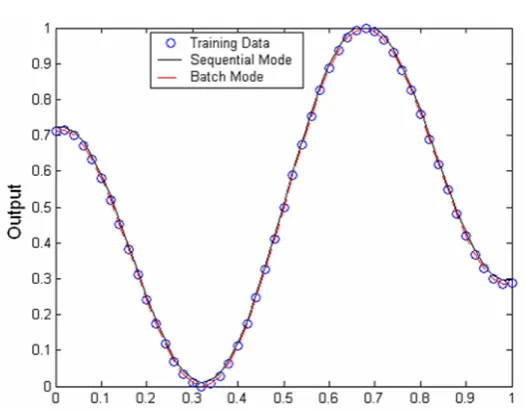
The network is trained with an adaptive gain with an initial value of unity for the gain parameter for all output as well as hidden nodes. In Figure 1(a) the network output (continuous curve) is shown against the training data points (circles) using the function
. The output of the network using constant unit gain value is also plotted in Figure 1(a) (dotted curve). The gain values for the five hidden nodes at the end of training are 1.5831, 0.9126, 1.9954, 1.9959 and 1.1594 respectively. The gain value for output node at the end of training is 1.9941.
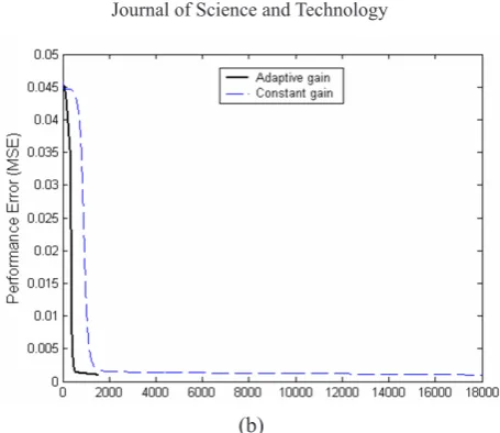
As shown in Figure 1(b) the speed of convergence of the proposed algorithm is high due to the modified gain values. The network required 1537 epochs to achieve the target error using the proposed adaptive gain algorithm in sequential mode, whereas using the same set of initial weight and biases the network required 17966 epochs to achieve the target error using constant unit gain value during training.
(b)
Figure 1 : Output of the neural network training to learn a cosine curve with and without using the adaptive gain algorithm in sequential mode of training (a), and convergence speed for the cosine function with and without using the adaptive gain
algorithm (b)
(b)
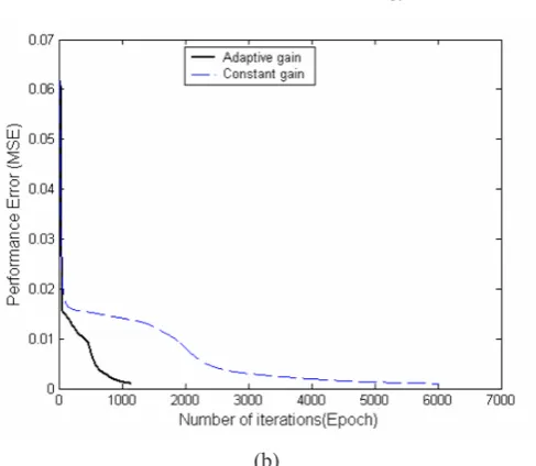
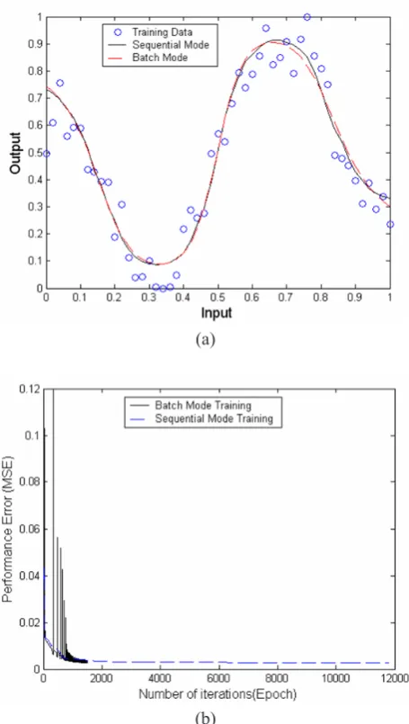
Figure 2 : Output of the neural network training to learn a sine curve with and with-out using the adaptive gain algorithm in sequential mode of training (a), and conver-gence speed for the sine function with and without using the adaptive gain algorithm
(b).
In Figure 2(a) the network output (continuous curve) is shown against the training data points (circles) y = x + sin(2*pi*x). The output of the network using constant unit gain value is also plotted in Figure 1(b) (dotted curve). The gain values for the five hidden nodes at the end of training are 1.3048, 0.7119, 1.9958, 1.5527 and 1.9985 respectively. The gain value for output node at the end of training is 1.9956. Again, the result showed that the speed of convergence is high due to the modified gain values. As shown in figure 2(b) the network required 1154 epochs to achieve the target error using the proposed adaptive gain algorithm in sequential mode, whereas using the same set of initial weight and biases the network required 6014 epochs to achieve the target error using constant unit gain value during training.
5 THE PROPOSED ALGORITHM USING BATCH MODE OF TRAINING
We propose an algorithm for changing the gain value adaptive for each node which is implemented for the batch mode of training. The following subsection describes the algorithm. The advantages of using an adaptive gain value have been explored. The gain update expressions as well as weight and bias update expressions for output and hidden nodes have already been derived in Section 3. The only difference is that in the batch mode of training the weight, bias and gain updation terms are calculated and summed for all the training examples. Then the weights, biases and gains are updated after one complete presentation of the entire training set. An epoch is said to be complete after the presentation of the entire training set. A sum squared error value is calculated after the presentation of the training set and compared with the target error. Training is done on an epoch-by-epoch basis until the sum squared error falls below the desired target value.
The following iterative algorithm is proposed by the authors for the batch mode of training. Weights, biases and gains are calculated and updated for the entire training set, which is being presented to the network.
For a given epoch, For each example, Step 1
Calculate the weight and bias and gain updation terms using the previously converged gain value.
Step 2
Use the weight and bias values calculated in Step (1) to calculate the gain updation value
Repeat Steps (1) and (2) for each example and sum all the weights, biases and gain updation terms.
6 VALIDATION ON THE ‘COSINE CURVE’ AND ‘SINE CURVE’ EXAMPLES USING BATCH MODE
The results of our proposed algorithm were validated on a standard feed forward neural network with one hidden layer having five hidden nodes. The training data set is created based on Bishop [10] by using the function
and where x є [0, 1]. The network
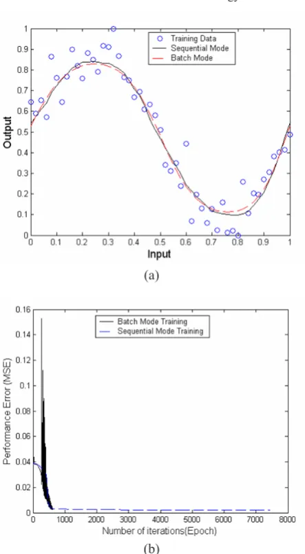
is trained using 0.3 as the learning rate value to achieve a target error equal to 0.001. The Gradient Descent training algorithm was employed in a batch mode with adaptive changes in weight, bias and gain values. The initial weight and bias values were chosen as small random numbers in the range [-1, +1]. The network is trained with an adaptive gain with an initial value of unity for the gain parameter for all output as well as hidden nodes. In Figure 3(a) the network output (continuous curve) is shown against the training data points (circles) using the function . The output of the network using constant unit gain value is also plotted in Figure 3(a) (dotted curve).
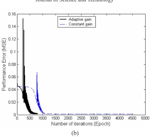
In Figure 3(b) the network required 803 epochs to achieve the target error using the proposed adaptive gain algorithm in batch mode, whereas using the same set of initial weights and biases the network required 4559 epochs to achieve the target error using unit gain value during training.
(b)
Figure 3 : Output of the neural network training to learn a cosine curve with and without using the adaptive gain algorithm in batch mode of training (a), and convergence speed for the cosine function with and without using the adaptive gain
algorithm in batch mode of training (b).
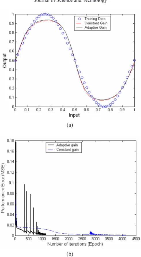
In Figure 4(a) the network output (continuous curve) is shown against the training data points (circles). The output of the network using constant unit gain value is also plotted in Figure 4(a) (dotted curve). Again, the result showed that the speed of convergence of the proposed algorithm is high due to the modified gain values. As shown in Figure 4(b) the network required 1148 epochs to achieve the target error using the proposed adaptive gain algorithm in batch mode, whereas using the same set of initial weight and biases the network required 4114 epochs to achieve the target error using constant unit gain value during training.
(a)
(b)
Figure 4 : Output of the neural network training to learn a sine curve with and without using the adaptive gain algorithm in batch mode of training (a), and convergence speed for the sine function with and without using the adaptive gain
7 EFFECT OF NUMBER OF HIDDEN NODES, TARGET NODES, TARGET ERROR AND INITIAL WEIGHT AND BIAS VALUES ON NETWORK TRAINING.
A standard feed forward neural network with one hidden layer having fifteen hidden nodes is now used to validate the results of our approach. The network is trained using the learning rate value of 0.3 and momentum value of 0.4 (in batch mode) to achieve a target error of 0.0001. The network was trained using the Gradient Descent training algorithm in both sequential and batch modes of training with adaptive changes in weight, bias and gain values. The network output for sequential mode (continuous curve) and batch mode (dotted curve) is shown against the training data points (circles) in Figure 5. It can be observed that outputs form both modes are almost the same and they overlap each other. Also, it can be seen that as the number of hidden nodes in the network is increased and the target error is reduced further, the trained network over fits the data and the curve passes through almost all the data points.
Figure 5 : Output of the neural network trained to learn a cosine curve using the adaptive gain algorithm in both sequential (continuous curve) and batch mode (dotted
curve) of training.
8 EFFECT OF NOISE
A standard feed forward neural network with one hidden layer having five hidden nodes is trained using a training data set which is created by using the function
and where x є [0,1], and adding 20%
random Gaussian noise in it. The network is trained using the learning rate value of 0.3 and momentum value of 0.4 (in batch mode) to achieve a target error of 0.002. The initial weights and biases are small normally distributed random numbers in the range [-1, +1]. The network was trained using the Gradient Descent training algorithm in both sequential and batch modes of training with adaptive changes in weight, bias and gain values. The network output for sequential mode (continuous curve) and batch mode (dotted curve) is shown against the training data points (circles) in Figure 6(a) and Figure 7(a). It can be observed that network trained in both modes perform in a similar way.
practical both situations data is generally inherently noisy. The output from both modes for both functions shows that the network is also successful in learning the target function when there is noise present in the data. The results strengthen our belief in the better working of the adaptive gain algorithm.
(a)
(b)
Figure 6 : Output of the neural network trained to learned a cosine curve with 20% random Gaussian noise using the adaptive gain algorithm in both sequential (continuous curve) and batch mode (dotted curve) of training (a), and convergence
(a)
(b)
Figure 7 : Output of the neural network trained to learned a sine curve with 20% random Gaussian noise using the adaptive gain algorithm in both sequential (continuous curve) and batch mode (dotted curve) of training (a), and convergence
speed for the sine function with using the adaptive gain algorithm in batch and sequential mode of training (b).
9 ADVANTAGES OF USING THE ADAPTIVE GAIN VARIATION
We proposed that the total learning rate value can be split into two parts – a local (nodal) learning rate value and a global (same for all nodes in a network) learning rate value. The value of parameter gain is interpreted as the local learning rate of a node in the network. The network is trained using a fixed value of learning rate equal to 0.3 which is interpreted as the global learning rate of the network. However, as the gain value was modified, the weights and biases were updated using the new value of gain. This resulted in higher values of gain which caused instability [7]. To avoid oscillations during training and to achieve convergence, an upper limit of 2.0 is set for the gain value. This will be explained in detail in our next publication. The method has been illustrated for Gradient Descent training algorithm using the sequential and batch modes of training. An advantage of using the adaptive gain procedure is that it is easy to introduce into a back-propagation algorithm and it also accelerates the learning process without a need to invoke solution procedures other than the Gradient Descent method. The adaptive gain procedure has a positive effect in the learning process by modifying the magnitude, and not the direction, of the weight change vector. This greatly increases the learning speed by amplifying the directions in the weight space that are successfully chosen by the Gradient-Descent method. However, the method will also be advantageous when using other faster optimisation algorithms such as Conjugate-Gradient method and Quasi-Newton method. These methods can only optimise an equivalent of the global learning rate (the step length). By introducing an additional local learning rate parameter, further increase in the learning speed can be achieved. Work is currently under progress to implement this algorithm using other optimisation methods.
10 CONCLUSION
While the back-propagation algorithm is used in the majority of practical neural networks application and has been shown to perform relatively well, there still exist areas where improvement can be made. We proposed an algorithm to adaptively change the gain parameter of the activation function to improve the learning speed. It was observed that the influence of variation in the gain value is similar to the influence of variation in the learning rate value. An algorithm has been proposed in this paper to change the gain value adaptively for each node.
The network also demonstrated the principles of over fitting vs. generalization as the number of hidden nodes in the network was increased and the target error was reduced further. The choice of normally distributed random numbers in the range [-1, +1] for the initial values of weights and biases in the network greatly speeded the training process.
In practical situations data is generally inherently noisy. A network trained with the adaptive gain algorithm in sequential as well as batch modes of training was also successful in learning the target function when there was noise present in the data. The results strengthen our belief in the better working of the adaptive gain algorithm.
ACKNOWLEDGMENT
The authors would like to thank Universiti Tun Hussein Onn Malaysia for supporting this research under the Short Term Research Grant.
REFERENCES
[1] Perantonis S. J. and Karras D. A., An Efficient Constrained Learning Algorithm with Momentum Acceleration. Neural Networks,
1995(8(2)): p. 237-249.
[2] Kamarthi S. V. and Pitner S., Accelerating Neural Network Training using Weight Extrapolations. Neural Networks, 1999. 12: p. 1285- 1299.
[3] Moller M. F., A Scaled Conjugate Gradient Algorithm for fast Supervised Learning. Neural Networks, 1993. 6(4): p. 525-533. [4] Lera G. and Pinzolas M., Neighborhood based Levenberg-
Marquardt Algorithm for Neural Network Training. IEEE
Transaction on Neural Networks, September 2002. 13(5): p. 1200- 1203.
[6] Hollis P. W., Harper J. S., and Paulos J. J., The Effects of Precision Constraints in a Backpropagation Learning Network. Neural Computation, 1990. 2(3): p. 363-373.
[7] Thimm G., Moerland F., and Fiesler E., The Interchangeability of Learning Rate an Gain in Back propagation Neural Networks. Neural Computation, 1996. 8(2): p. 451-460.
[8] Looney C. G., Stabilization and Speedup of Convergence in Training Feed Forward Neural Networks. Neurocomputing, 1996. 10(1): p. 7-31.
[9] Eom K., Jung K., and Sirisena H., Performance Improvement of Back propagation algorithm by automatic activation function gain tuning using fuzzy logic. Neurocomputing, 2003. 50: p. 439-460.
[10] Bishop C. M., Neural Networks for Pattern Recognition. 1995: Oxford University Press.