Mining Frequent Subgraph by Incidence Matrix
Normalization
Jia Wu
Department of Computer Science, Yangzhou University, Yangzhou, China
Ling Chen*
Department of Computer Science, Yangzhou University, Yangzhou, China National Key Lab of Novel Software Tech, Nanjing University, Nanjing, China
Email: [email protected]
Abstract—Existing frequent subgraph mining algorithms
can operate efficiently on graphs that are sparse, have vertices with low and bounded degrees, and contain well-labeled vertices and edges. However, there are a number of applications that lead to graphs that do not share these characteristics, for which these algorithms highly become inefficient. In this paper we propose a fast algorithm for mining frequent subgraphs in large database of labeled graphs. The algorithm uses incidence matrix to represent the labeled graphs and to detect their isomorphism. Starting from the frequent edges from the graph database, the algorithm searches the frequent subgraphs by adding frequent edges progressively. By normalizing the incidence matrix of the graph, the algorithm can effectively reduce the computational cost on verifying the isomorphism of the subgraphs. Experimental results show that the algorithm has higher speed and efficiency than that of other similar ones.
Index Terms—graph; incidence matrix; isomorphism; data
mining
I. INTRODUCTION
Data mining is the process of automatically extracting new and useful knowledge hidden in large datasets. In recent years, the study on semi-structured and structured data is showing more and more practical value [1] and there has been an increased interest in developing data mining algorithms on such data like graphs. The problem of frequent subgraph mining arises naturally in a number of different application domains including network intrusion [2,3], semantic web [4], behavioral modeling [5,6] , VLSI reverse engineering [7], link analysis [8,9.10,11] , and chemical compound classification [12-15]. Moreover, they can be used to effectively model the structural and relational characteristics of a variety of datasets arising in areas of physical sciences and chemistry such as fluid dynamics, astronomy, structural mechanics, and ecosystem modeling, life sciences such as genomics, proteomics, pharmacogenomics, and health informatics, and information security such as information assurance, infrastructure protection, and terrorist-threat
prediction/identification. We can solve these problems by graph mining method.
Frequent subgraphs mining is to choose subgraphs that meet a certain support threshold from graph data set and it is the base for the research of graph clustering, graph classification, graph query and restricted graph mining. However, the traditional mining methods that based on non-structured data such as frequent-item set mining and sequential-pattern mining have not been equal to the mining work on semi-structured and structured data such like graph. Algorithm studies on frequent graph mining were never stopped. Earlier frequent subgraph mining algorithms like SUBDUE [16] approximate method which can only get approximate result. In SUBDUE, since graphs are compressed as minimum description length and adopting heuristic searching method to mine frequent subgraphs, it can’t guarantee the integrality of result. In 2000, Inokuchi and Kuramochi brought Apriori method into subgraph mining and therefore AGM [17] and FSG [18, 19] were proposed. AGM and FSG can enumerate all the subgraphs by increasing vertexes and edges progressively. This approach opened the precedent of putting traditional data mining methods into subgraph mining research. In recent years, algorithms that based on FP-growth like gSpan [20] and FFSM [21] have achieved higher efficiency. Each algorithm has respectively made distinct improvement on the two efficiency-related aspects, that is, subgraph isomorphism judgment and the strategy of frequent subgraph extension. In AGM, FSG, FFSM and their improvements [22,23], graphs are denoted by adjacency matrix and find isomorphic graphs by adjacency matrix code. However, even the most efficient algorithm FFSM still need matrix join and extension operations which made the time complexity for subgraph extension be O( n
n
m2⋅ ⋅2 ) [24]. The algorithm gSpan and its improvements[26] denote graphs in the form of the minimum DFS code, which is the base for its edge extension strategy, yet the time complexity for isomorphic graphs judgment is still as high as O(2n).
graphs that are sparse, contain a large number of relatively small connected components, have vertices with low and bounded degrees, and contain well-labeled vertices and edges. However, there are a number of applications that lead to graphs that do not share these characteristics, for which these algorithms highly become inefficient. In order to overcome these shortages, we propose a new frequent subgraph mining algorithm FSMA (frequent subgraph mining algorithm) in this paper. The algorithm uses incidence matrix to represent the labeled graphs and to detect their isomorphism. Starting from the frequent edges from the graph database, the algorithm identifies the frequent subgraphs by adding edges progressively. By normalizing the incidence matrix of the graph, the algorithm can effectively reduce the computational cost on verifying the isomorphism of the subgraphs. Experimental results show that the algorithm has higher speed and efficiency than that of other similar ones.
The remainder of the paper is organized as follows. In Section 2, we define the labeled graph and their isomorphism. Section 3 presents the method of normalize the incidence matrixes of labeled graph. Framework of the frequent subgraph mining algorithm FSMA is proposed in Section 4. Experimental results are shown and analyzed in Section 5, and Section 6 concludes the paper.
II. LABELED GRAPHS AND THEIR ISOMORPHISM
Definition 1 (Labeled Graph [25] and Labeled Graph Data Set) A labeled graph G is denoted by a quadruple G=(V(G),E(G),L(V(G)),L(E(G))), where V(G)={v1,v2,…,vn} is the graph vertexes set and E(G)={ek=(vi,vj)|vi,vj∈V(G)}⊆V×V is the graph edges set, L(V(G))={lb(vi)|∀vi∈V(G)} is the graph vertexes’ labels set, L(E(G))={lb(ek)|∀ ek∈E(G)} is the graph edges’ labels set. Let G1, G2, G3,…,Gu be labeled graphs, set GDB={G1,G2,G3,…,Gu} is called a labeled graph data set.
Definition 2 (Identical Labeled Vertexes Set and Identical Labeled Edges Set) For a vertexes set SV of a labeled graph G, if all the vertexes in SV have the same label lv, i.e. for every vi
∈
SV , lb(vi) = lv , then SV is called an identical labeled vertexes set and is denoted as SV(lv). Similarly, for an edges set SE of a labeled graph G, if all the edges in SE have the same label le, i.e. for every ei∈
SE , lb(ei) =le, then SE is called an identical labeled edges set and is denoted as SE(le).In this paper, in order to identify the vertexes (edges), we assign an index to each vertex (edge) in an identical labeled vertexes (edges) set.
Definition 3 (Labeled Graph Isomorphism [26, 27]) Given two labeled graphs G and G', if there exists a mapping function f : V(G)→V(G'), which satisfies: (1) ∀ vi ∈ V(G), lb(vi)=lb( f (vi));
(2) ∀ (vi,vj) ∈ E(G),( f (vi), f (vj)) ∈ E(G'), lb((vi,vj))=lb( f (vi), f (vj)), then we call G and G' isomorphic graphs, and denote them as G≅G'.
Definition 4 (Labeled Isomorphic Subgraph) Given two labeled graph G and H, if H' is a subgraph of H and H' ≅ G, then G is the labeled isomorphic subgraph of H, and is denoted as G⊆H.
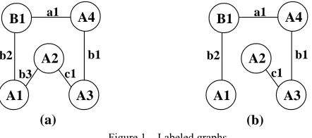
In Fig. 1, (b) is a labeled isomorphic subgraph of Fig. 1 (a).
Definition 5 (Support and Frequent Subgraph) Given labeled graph data set GDB={G1,G2,G3,…,Gu} and labeled graph G', support of G’ in GDB is defined as sup(G')=|{H| H∈GDB and G' ⊆H}| which is the number of graphs in GDB of which G' is a labeled isomorphic subgraph. A frequent subgraph of GDB is a graph whose support is no less than a predefined threshold minsup.
Definition 6 (Maximum Frequent Subgraph) Suppose G' is a frequent subgraph of GDB, if for any labeled graph G which satisfies G'⊆G, G is not a frequent subgraph of GDB, then we call G' a maximum frequent subgraph of GDB.
B1 A4
A3 A1
A2 a1
b1 b2
b3 c1
B1 A4
A3 A1
A2 a1
b1 b2
c1
(a) (b)
Figure 1. Labeled graphs
The goal for frequent subgraph mining is to find all the maximum subgraphs that satisfy the threshold minsup in a graph data set GDB.
Ⅲ. GRAPH’S INCIDENCE MATRIX AND ITS NORMALIZATION
Important part of frequent subgraph mining is the strategy to represent the graphs in appropriate data structure, so that the algorithm could take feasible graph extension strategy to enumerate all frequent subgraphs. Since verifying the isomorphism of graphs is a NP-complete problem, it should make an effective way to normalize these graphs in order to reduce the complexity on isomorphism detecting. As a representation of graphs, incidence matrix has the characteristics of intuitionist and being easy compressed. Therefore, we use incidence matrix to denote graphs in our algorithm FSMA. For easy normalization as well as subgraph extension, we also present the definition of normalized format of incidence matrix.
A. Graph’s Incidence Matrix
Given a connected labeled graph
G=(V(G),E(G),L(V(G)),L(E(G))), where
L(V(G))={A1,A2,…,Ar}(r ≤ m) and
L(E(G))={B1,B2,…,Bs}(s≤n). Let SV(Ai)={vi1,vi2,…,vimi} be an identical labeled vertexes set with vertexes of the
same label Ai and
∑
=
=
r i
i m
m
1
, SE(Bj)={ej1,ej2,…,ejnj} be
label Bj and
∑
=
=
s j
j n
n
1
. For labeled graph G, its
incidence matrix M is an m×n matrix, where each row represents a vertex and each column represents an edge. The entry for row v and column e is 1 if e is incident with v and 0 otherwise. Namely, matrix element v
e
M can be defined as:
v e
M =
⎩ ⎨ ⎧
v e
v e
ith incident w not
is 0
ith incident w is
1
.
The rows of the matrix are divided into several blocks each of which represents the rows of one identical row set. Similarly, the columns of the matrix are also divided into groups representing the identical column sets. Table
Ⅰ shows a common format for incidence matrix of a labeled graph.
TABLE Ⅰ.
INCIDENCE MATRIX OF A LABELED GRAPH
For a connected labeled graph G, its incidence matrix is obviously not unique. Since the vertexes (or edges) sharing the same label could be arranged in different orders in the matrix, different forms of incidence matrix for G could be produced. In order to detect the isomorphism of the subgraphs, these incidence matrixes should be transformed into a normalized form which is unique for a connected labeled graph.
B The Algorithm for Incidence Matrix Normalization Here, we propose an algorithm named IM-Norm to transform an incidence matrix of a labeled graph G into the normalized one. The input for the algorithm is an incidence matrix M of a k-edge candidate subgraph g(G, k) in G, and the output is g(G, k)’s normalized incidence matrix MS. The algorithm consists of two steps, the first step performs normalization on the rows of the matrix (namely, graph’s vertexes), and then the columns (i.e. graph’s edges) normalization. In the row (column) normalization, rows (columns) are rearranged according to their row (column) labeled vectors and the binary numbers they represented.
Definition 7 For a vertex vk (i.e. row k in the incident matrix) in identical vertex set SV(Ai), its labeled vector is defined as Ck=(ckb1, ckb2, …, ckbs), where ckbj is the
number of edges in the identical labeled edges set SE(Bj ).
Definition 8 For an edge ek (i.e. column k in the
incident matrix) in identical edge set SE(Bj), its labeled vector is defined as Dk=(dka1, dka2, …, dkar), where dkai is
the number of vertexes in the identical labeled vertexes set SV(Ai).
Since each entry in the incidence matrix is a binary bit, each row (column) represents a binary number. We denote the binary number the kth row (column) represented as rcodek (ccodek).
The algorithm consists of two steps each of which performs rows or columns normalization. In the rows normalization, the algorithm sorts the rows in an identical labeled row set according to their labeled vectors in lexicographic order
p
. However, if labeled vectors of two rows in the same identical row set are equivalent, they will be sorted according to the values of the binary numbers they represented.The algorithm performs the column normalization in a similar way. Suppose labeled graph G has r identical labeled row sets and s identical labeled column sets, framework of the algorithm IM-_Norm is as follows:
Algorithm 1 IM_Norm
Input: Candidate subgraph’s incidence matrix M Output: Candidate subgraph’s normalized incidence matrix MS
1: for round=1 to 2 do
/* two steps of rows & columns normalization*/ 2: for i= 1 to r do /* rows normalization */ 3: for k=i1 to imi do
/* sort rows in row block of SV(Ai) */ 4: for j= k+1 to imi do
5: if
j k
C
C
p
then6: exchange rows k and j
7: else if (Ck =Ck+1) and
(rcodek<rcodek+1) then
8: exchange rows k and j
9: endif
10: endif 11: endfor j 12: endfor k 13: endfor i
14: for i= 1 to s do /* columns normalization */ 15: for k=j1 to jnj do
/* sort columns in column block of SE(Bj) */ 16: for j= k+1 to jnj do
17: if
D
kp
D
j then18: exchange columns k and j
19: else if (Dk =Dk+1) and (ccodek <ccodek+1) then
20: exchange columns k and j 21: endif
24: endfor k 25: endfor i 26: endfor round 27: return(MS)
The first part of IM_Norm (lines 2 ~ 13) is to normalize the rows (i.e. vertexes) of matrix M by arranging the rows sharing the same vertex label in lexicographic order. However, if labeled vectors of two rows’ in the same identical row set are equivalent (lines 7 ~ line 9), they will be sorted according to the values of the binary numbers they represented.
The second part of IM_Norm (lines 14 ~ line 26) is to normalize all the columns (i.e. edges) of matrix M in a similar way.
The algorithm reiterates such row and column normalization once more to get the normalized form of the incidence matrix MS which will be used in graph isomorphism detection.
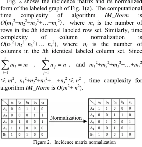
Fig. 2 shows the incidence matrix and its normalized form of the labeled graph of Fig. 1(a). The computational time complexity of algorithm IM_Norm is O(m12+m22+m32+…+mr2), where mi is the number of rows in the ith identical labeled row set. Similarly, time complexity of column normalization is O(n12+n22+n32+…+ns2), where ni is the number of columns in the ith identical labeled column set. Since
∑
=
=
r i
i m
m
1
,
∑
=
=
s j
j n
n
1
, and m12+m22+m32+…+mr2
≤m2, n12+n22+n32+…+ns2≤n2 , time complexity for algorithm IM_Norm is O(m2+ n2).
Figure 2. Incidence matrix normalization
Ⅳ. FREQUENT SUBGRAPH MINING ALGORITHM FSMA
The goal of algorithm FSMA is to find all the subgraphs which have a certain minimum support in a given graph data set GDB. FSMA uses the normalized incidence matrix to present the subgraphs. By scanning GDB, FSMA first finds all the frequent edges, which is also called 1-edge frequent subgraphs. Then the algorithm extends the 1-edge frequent subgraphs by adding frequent edges on them to get 2-edge frequent subgraphs. Repeating this procedure of subgraph extension until no more frequent subgraphs being generated. The advantage of FSMA is that it extends the frequent subgraphs by only adding the frequent edges instead of enumerating all the subgraphs in the graphs. This pruning technique can greatly reduce the time complexity.
Table Ⅱ lists the parameters used in FSMA.
TABLE Ⅱ.
PARAMETERS USED IN ALGORITHM FSMA
Parameter Meaning F(k) number of k-edge frequent subgraphs
Ne set of edges ewith subgraph g(G, k)
∉
g(G, k) but connectedTFG(G, k) set of k-edge candidate subgraphs in graph G TFGC(K) set of k-edge candidate subgraphs FG(G, K) set of k-edge frequent subgraphs in graph G
FGS(GDB) set of 1-edge to k-edge frequent subgraphs
gn(G, k) normalized incident matrix of a k-edge subgraph in graph G Freq_gn(G,
k) frequency of gn(G, k)
We use "gn(Gi , k)◇e" to denote the operation of extending the subgraph represented by gn(Gi , k) with edge e. Framework of algorithm FSMA is as follows:
Algorithm 2 FSMA
Input: Graph data set GDB={G1, G2, …,Gn}, the minimum support threshold minsup Output: Frequent subgraph data set FGS(GDB)
1: scan GDB, generate frequent edges; number of frequent edges is saved in F(1) 2: for i=1 to u do /* for each Gi in GDB */ 3: delete unfrequent edges in Gi 4: FG(Gi, 1)←{ frequent edges in Gi } 5: endfor
6: k←1
7: while F(k)>0 do
8: for i=1 to n do /* for each Gi in GDB */ 9: TFG(Gi, k+1)=Φ
10: for each k-edge frequent subgraph gn(Gi, k) ∈FG(Gi, k) do
11: Ne←{ set of edges e
∉
g(G, k) but connected with subgraph g(G, k) } 12: for each e in Ne do13: gn( Gi, k+1)= gn(Gi , k)◇e
14: if gn (Gi, k+1)
∉
in TFG(Gi, k+1) then15: TFG(Gi, k+1)=
TFG(Gi, k+1)∪{gn(Gi, k+1)} 16: endif
17: endfor e 18: endfor 19: endfor i
20: for i=1 to n do /* for each Gi in GDB */ 21: for each gn(G, k+1) in TFG(Gi, k+1) do 22: if gn(G, k+1)
∉
TFGC(k+1) then 23: TFGC(k+1)= TFGC(k+1) {gn(G, k+1)} ∪ 24: Freq_gn(G, k+1)= 125: else
26: Freq_gn(G, k+1)=Freq_gn(G, k+1)+1 27: endif
29: endfor i 30: F(k+1)=0;
31: for each gn(G, k+1) in TFGC(k+1) do 32: if Freq_gn(G, k+1)> minisup then 33: FGS(GDB)= FGS(GDB)∪{gn(G, k+1)} 34: F(k+1)= F(k+1)+1
35: endif 36: endfor
37: for i=1 to n do /* for each Gi in GDB */ 38: FG(G, k+1)=Φ
39: for each gn(Gi, k+1) in TFGC(k+1) do 40: if gn(Gi, k+1)∈FGS(GDB)
41: FG(G, k+1)=FG(G, k+1)∪{gn(G, k+1)} 42: endif
43: endfor 44: endfor i 45: k←k+1 46: wend
47: delete non-maximum frequent subgraphs in FGS(GDB)
48: Return (FGS(GDB))
The first part of FSMA (lines 1 ~ 5) is the initial stage of the algorithm. In this stage, the algorithm first scans GDB and generates frequent edges and computes the number of those frequent edges. For each graph Gi, the algorithm builds a set FG(Gi, 1) consisting of all frequent edges in Gi. Lines 3 and 4 delete all unfrequent edges in each graph and update the graph data set. Lines 6 to 46 perform subgraph extension by progressively adding frequent edges on the existing frequent subgraphs. In each iteration of the extension procedure, a set of (k+1)-edge frequent subgraphs in graph Gi , which is named FG(G, k+1), can be obtained based on FG(G, k). In lines 8 to 19, all the (k+1)-edge candidate subgraphs in each graph Gi are generated by adding frequent edges on the k-edge frequent subgraphs in graph Gi . Line 13 generates a (k+1)-edge candidate subgraph gn(Gi, k+1) by adding an edge e in Ne on k-edge frequent subgraph gn(Gi , k). This extension operation “◇” is implemented by normalizing the incidence matrixes of the subgraphs using algorithm IM_Norm. All the k-edge candidate subgraphs of graph Gi are saved in set TFG(Gi, k). In lines 20 to 29, the candidate subgraphs in TFG(Gi, k), i= 1,2,…,n, are jointed into set TFGC(k+1) and their frequencies are calculated. In lines 30 to 36, the frequent (k+1)-edge subgraphs are selected from TFGC(k+1) and saved into the set FGS(GDB). In the meanwhile, number of (k+1)-edge frequent subgraphs, denoted by F(k+1), are calculated. Lines 37 to 46 construct a set FG(G, k+1) for each graph G in GDB to record the (k+1)-edge frequent subgraphs in G . Set FG(G, k+1) will be used to generate the (k+2)-edge candidate subgraphs in the next iteration. The iteration of subgraph extension will end when F(k)=0 which indicates no frequent subgraph with more edges could be produced. In lines 14, 22 and 40, isomorphism of subgraphs should be detected when searching a subgraph in the graph set. Since the algorithm uses the normalized incidence matrix, it can detect the isomorphism very efficiently. In the algorithm, since the
frequent subgraphs are extended progressively from 1-edge subgraphs and their incident matrixes are normalized when they are generated by subgraph extension, it is not necessary to normalize each graph’s incidence matrix in the initial stage.
Ⅴ. EXPERIMENT RESULTS AND PERFORMANCE ANALYZE
In this section, we report our experiments that validate the effectiveness and efficiency of our algorithm FSMA. We test algorithm FSMA on a 2.80GHz Intel Pentium Ⅳ
PC with 256 MB main memory, running Windows XP Professional SP2. A comparative study also has been conducted between FSMA and SLAGM [22] on their performance on random graphs data set. Those graphs are generated under certain controlling parameters and are saved in the forms of incidence matrix and adjacency matrix respectively. Both FSMA and SLAGM are coded using VC++ 6.0. Table Ⅲ lists the parameters used in the experiments.
TABLE Ⅲ.
PARAMETERS IN THE EXPERIMENTS
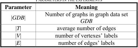
Parameter Meaning
|GDB| Number of graphs in graph data set GDB |T| average number of edges |V| number of vertexes’ labels |E| number of edges’ labels
All the experimental results show that FSMA and SLAGM have the same quality of results but FSMA has obviously higher processing speed than SLAGM. Fig. 3, 4 and 5 show the runtime comparisons of two algorithms. In these experiments, the parameters are set as follows: in Fig. 3, |GDB|=200, |T|=20, |V|=17, |E|=11, in Fig. 4, |GDB|=200, minsup=10%, |V|=23, |E|=15, in Fig. 5, |T|=20, minsup=10%, |V|=19, |E|=13.
Fig. 3 shows runtime comparison between SLAGM and FSMA under different values of minsup. From Fig. 3, we can see that efficiency of FSMA is superior to SLAGM. When minsup decreases, FSMA is even more efficient. This is because SLAGM extends a (k+1)-vertex subgraph based on two k-vertex subgraphs that share the common (k-1)-vertex subgraphs, it consumes large amount of time to discover such pairs of k-vertex subgraphs. Since FSMA extends the subgraph directly by adding a frequent edge in each iteration, it requires much less computation time.
0 20 40 60 80 100
0 2 4 6 8 10 12 14 Minsup(%)
Run
Tim
e(s
)
Figure 3. Runtime comparison between SLAGM and FSMA under different minisup
Fig. 4 shows runtime comparison between SLAGM and FSMA under different graph scales |T| which is measured by the average number of edges of the graphs in GDB. From Fig. 4 we can see that FSMA is always faster than SLAGM under different |T| and FSMA is even more efficient when |T| increases. This is because subgraph extensions on large scaled graphs spend much more computation time in SLAGM.
0 50 100 150 200 250 300 350
0 5 10 15 20 25 30 35 |T|(个)
Run
Tim
e(s
)
SLAGM FSMA
Figure 4. Runtime Comparison between SLAGM and FSMA under Different |T|
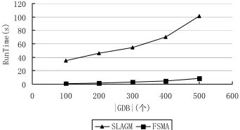
Fig. 5 shows runtime comparison between SLAGM and FSMA under different |GDB|, which is the umber of graphs in graph data set GDB. From Fig. 5, we can see that the speed by FSMA could be 10 ~ 12 times of that by SLAGM when the number of graphs increases.
0 20 40 60 80 100 120
0 100 200 300 400 500 600 |GDB|(个)
RunTime(
s)
SLAGM FSMA
Figure 5. Runtime Comparison between SLAGM and FSMA under Different |GDB|
Ⅵ. CONCLUSIONS
An algorithm FSMA to find frequent subgraphs in large labeled graph database is presented. FSMA uses incidence matrix to represent the labeled graphs and to detect their isomorphism. Starting from the frequent edges from the graph database, the algorithm searches for the frequent subgraphs by progressively adding frequent edges on the existing frequent subgraphs. By normalizing the incidence matrix of the graph, the algorithm can effectively reduce the computational cost on verifying the isomorphism of the subgraphs. Experimental results show that the algorithm has higher speed and efficiency than that of other similar ones.
ACKNOWLEDGMENT
This research was supported in part by the Chinese National Natural Science Foundation under grant No.
60673060, Natural Science Foundation of Jiangsu Province under contract BK2008075, and the Graduated Education Research Foundation of Jiangsu Province.
REFERENCES
[1] D. Cook, L. Holder. Mining Graph Data. John Wiley & Sons, 2007: 99-115.
[2] Lee,W. and Stolfo, S.J. 2000. A framework for constructing features and models for intrusion detection systems. ACM Transactions on Information and System Security, 3(4):227–261.
[3] Ko, C. 2000. Logic induction of valid behavior specifications for intrusion detection. In IEEE Symposium on Security and Privacy (S&P), pp. 142–155.
[4] Berendt, B., Hotho, A., and Stumme, G. 2002. Towards semantic web mining. In International Semantic Web Conference (ISWC), pp. 264–278.
[5] Wasserman, S., Faust, K., and Iacobucci, D. 1994. Social network analysis: Methods and applications. Cambridge University Press.
[6] Mooney, R.J.,Melville, P., Tang, L.R., Shavlik, J., Castro Dutra, I. de, Page, D. et al. 2004. Relational data mining with inductive logic programming for link discovery. In AAAI Press/The MIT Press, pp. 239–255.
[7] Yoshida, K. and Motoda, H. 1995. CLIP: Concept learning from inference patterns. Artificial Intelligence, 75(1):63– 92.
[8] Jensen, D. and Goldberg, H. (Eds.). 1998. Artificial Intelligence and Link Analysis Papers from the 1998 Fall. Symposium. AAAI Press.
[9] Kleinberg, J.M., Kumar, R., Raghavan, P., Rajagopalan, S., and Tomkins, A.S. 1999. The Web as a graph: Measurements, models and methods. Lecture Notes in Computer Science, 1627:1–17.
[10]Kleinberg, J.M. 1999. Authoritative sources in a hyperlinked environment. Journal of the ACM (JACM), 46(5):604–632.
[11]Palmer, C.R., Gibbons, P.B., and Faloutsos, C. 2002. ANF: A fast and scalable tool for data mining in massive graphs. In Proc. of the 8th ACM SIGKDD Internal Conference on Knowlege Discovery and Data Mining (KDD-2002) Edmonton, AB, Canada, pp. 81–90.
[12]Dehaspe, L., Toivonen, H., and King, R.D. 1998. Finding frequent substructures in chemical compounds. In Proc. of the 4th ACM SIGKDD International Conference on Knowledge Discovery and Data Mining (KDD-98), R. Agrawal, P. Stolorz, and G. Piatetsky-Shapiro (Eds.), AAAI Press, pp. 30–36.
[13]Kramer, S., De Raedt, L., and Helma, C. 2001. Molecular feature mining in HIV data. In Proc. of the 7th ACM SIGKDD International Conference on Knowledge Discovery and Data Mining (KDD-01), pp. 136–143. [14]Gonzalez, J., Holder, L.B. and Cook, D.J. 2001.
Application of graph-based concept learning to the predictive toxicology domain. In Proc. of the Predictive Toxicology Challenge Workshop.
[15]Deshpande, M., Kuramochi, M., and Karypis, G. 2003. Frequent sub-structure based approaches for classifying, chemical compounds. In Proc. of 2003 IEEE International Conference on Data Mining (ICDM), pp. 35–42.
[16]Holder LB, Cook DJ, Djoko S. Substructures discovery in the subdue system. Proc. of the AAAI’94 Workshop Knowledge Discovery in Databases, 1994: 169−180. [17]Inokuchi A, Washio T, Okada T, Motoda H. Applying
[18]Kuramochi M, Karypis G. An Efficient Algorithm for Discovering Frequent Subgraphs. Proc. of the IEEE Trans. Knowl. Data Eng., 2004, 16(9):1038-1051.
[19]Kuramochi M, Karypis G. Frequent subgraph discovery. Proc. of ICDM, 2001.
[20]Yan Y, Han J. gSpan: Graph-Based substructure pattern mining. Proc. of ICDM, 2002.
[21]J. Huan, W. Wang, J. Prins. Efficient Mining of Frequent Subgraphs in the Presence of Isomorphism. Proc. of ICDM, 2003.
[22]Li Yuhua, Luo han-guo, Sun Xiao-lin. A Frequent Subgraph Discovery Algorithm Based on Apriori’s Idea, Comper Engineering & Science, 2007, 29 (4): 84-87. [23]Phu Chien Nguyen, Takashi Washio, Kouzou Ohara,
Hiroshi Motoda. Using a Hash-Based Method for Apriori-Based Graph Mining. Proc. of PKDD, 2004.
[24]LI Xian-Tong, Li Jian-zhong, Gao Hong. An Efficient Frequent Subgraph Mining Algorithm. Journal of Software. 2007, 18 (10):2469-2480.
[25]Wang Yan-Hui, Wu Bin, Wang Bai. Survey of Frequent Subgraph Mining. Computer Science. 2005, 32 (10): 193-197.
[26]Wang Chen, Shi Bo-le, Wang Wei. Structured Data Mining and Processing Problems Research. 2005.
[27]Yin Jian-hong, Wu Kai-ya. Graph Theory and Algorithms. University of Science and Technology of China Press. 2003.
J. Wu was born in Yancheng, Jiangsu Province, P.R.China, in July 21, 1984. He received B. Sc degree in computer science from Yangzhou University, P.R. China in 2006. He is currently a M. Sc candidate in the Institute of Information Science and Technology, Yangzhou University, P.R.China.
His research interest includes data mining, bioinformatics and parallel processing.
L. Chen was born in Baoying, Jiangsce, P.R.China, in
September 10, 1951. He received B. Sc degree in mathematics from Yangzhou Teachers’ College, P.R. China in 1976.
He is currently professor of computer science, and the dean of Information Technology College, Yangzhou University, Jiangsu Province, P.R. China. He has published more than 120 papers in journals including IEEE Transactions on Parallel and Distributed System, Journal of Supercomputing, The Computer Journal. In addition, he has published over 100 papers in refereed conferences. He has also co-authored/co-edited 5 books (including proceedings) and contributed several book chapters. His research interest includes data mining, bioinformatics and parallel processing.