ENERGY MANAGEMENT OF SOLAR THERMAL ENERGY DRIVING ORC AND TDC

Abed et al. World Journal of Engineering Research and Technology

ENERGY MANAGEMENT OF SOLAR THERMAL ENERGY DRIVING

ORC AND TDC

K. A. Abed*1, Amr M. A. Amin2, Adel A. El-Samahy2 and Abdullah M. A. Shaaban1

1

Mechanical Eng. Depart., National Research Centre (NRC).

2

Electrical Eng. Depart., Faculty of Engineering, Helwan University.

Article Received on 03/01/2019 Article Revised on 24/01/2019 Article Accepted on 15/02/2019

ABSTRACT

The present work aims to manage the thermal energy stored from

concentrated solar power (CSP) research plant, in order to obtain the

best operating condition of CSP system. This plant consists of solar

collector field of 120 kW peak thermal capacity, thermal storage tank

with 3 tons of therminol-66 oil, an organic rankine cycle (ORC) of 8

kW nominal electric power production capacity, and thermally driven absorption chiller

(TDC) of 35 kW cooling capacity. The system was modeled mathematically then calculated

using engineering equation solver (EES) software in order to analyze the performance at

similar conditions to the real ones to ensure the feasibility of the presented study. When

increasing the input thermal power for both ORC and TDC, the kWh cost decreases. The

lowest price for ORC kWh is 1.131 $/kWh when 100% of the stored thermal power is used

by ORC to generate electricity. Also, the lowest price for TDC kWh is 0.1214 $/kWh when

100% of the stored thermal power is directed to the TDC. To compromise between both ORC

and TDC, The best operating condition is obtained when about 45.83% from stored thermal

power is used for ORC and 54.17% is used for TDC. In this case, the cost of electrical kWh

from ORC is about 1.26 $, while the cost of refrigerant kWh from TDC is about 0.126 $.

KEYWORDS: Renewable Energy, Concentrated Solar Power System, Organic Rankine Cycle, Thermally Driven Absorption Chiller.

Journal of Engineering Research and Technology

World

WJERT

www.wjert.org

*Corresponding Author K. A. Abed

Mechanical Eng. Depart.,

National Research Centre

INTRODUCTION

Nowadays, energy is one of the most basic and crucial elements upon which to base a life and

an economy. Energy is very important for daily tasks in homes, schools, hospitals, business,

transport applications, industries and countless other places. Most of energies come from

burning fossil fuels like oil, coal and natural gas which are called conventional or traditional

energy resources.[1] Since crisis for USA of the mid 1970's, the world’s industrialized nations

look at renewable energy sources (RES) as a supplement to providing the projected increase

in energy demand in their nations in addition to increase awareness of the effects of

emissions from fossil fuel power plants to the humans and environment. Governments in

industrial countries are currently made debating and enacting pollution control regulations

into laws.[2]

Solar energy is a source, which can be exploited in two main ways to generate power: direct

conversion into electric energy using photovoltaic (PV) panels and by means of a

thermodynamic cycle. In CSP plants it is the sun’s thermal energy to be stored, whereas in

PV applications it is the electrical energy to be stored in batteries. Umberto Desideri et al

studied the performance of concentrated solar power plants equipped with molten salts

thermal storage to cover a base load of 3 MWe. The electricity production of the CSP

facilities has been analyzed and then compared with the electricity production of PV plants.[3]

Wisam Abed et al presented a detail dynamic model of a 50 MWe parabolic trough power

plant.[4] The parabolic trough power plant is modeled using advanced process simulation

software (APROS). During summer days, the plant typically operates for 10–12 hr a day on

solar energy at full-rated electric output. Furthermore, the thermal storage system enables the

parabolic trough power plant to produce a constant electrical power rate, despite the slight

fluctuations in the solar radiation. The thermal storage system after sunset continues

approximately 7.5 hr for covering electrical power of 48 MWe until the thermal storage

energy is completely depleted.

Monica Borunda et al presented a study of a small CSP plant coupled to an ORC with

thermal energy storage.[5] Molten salts could be a very good possibility to highly increase the

solar fraction but it is much more expensive. On the other hand concrete storage is much

cheaper but with less heat capacity. However phase change materials may be a good and

Rady et al studied a small scale multi-generation solar plant which consists of solar collector

field, thermal storage tank, an ORC, and TDC.[10] This article reported on the plant layout,

thermodynamic analysis, solar field design, ORC and TDC integration, thermal storage

system, and control system and operation strategy. The plant is modeled and analyzed using

parabolic trough (PTC) and Linear Fresnel collectors (LFR) at different operation modes in

typical winter and summer days. The use of LFR solar collectors results in reduction in the

operation hours of ORC and TDC by about 50% and 30%, respectively.

Mohamed H. Ahmed et al also studied solar power plant consisting of ORC and absorption

chiller.[7] This paper presented a numerical simulation for the performance of solar thermal

power plant which consists of 190 m2 of concentrated PTC with a storage tank and an ORC.

A study of the operating parameters of the PTC performance was presented in this paper. The

plant used the Therminol-VP1 as a storage media and also as a heat transfer fluid with flow

rate ranges from 0.9 to 1.8 kg/s for the solar collectors. It’s used also as a heat source for the

ORC and the absorption chiller with a flow rate range from 0.3 to 0.9 kg/s. The model studied

also the effect of these operating modes on the plant performance. The simulation model

proves that the PTC produces a maximum thermal power of about 70 and 115 kW in winter

and summer respectively.

Mustapha Merzouk et al studied the performance of a single effect solar absorption cooling

system.[6] A dynamic simulation model, for a solar powered absorption cooling system was

developed, and validated using measured data. Yeung et al, designed and installed a solar

driven absorption chiller at the University of Hong Kong, this system included 4.7 kW

absorption chiller, flat plate solar collectors with a total area of 38.2 m², water storage tank

and the rest of the equipment. They reported that the collector efficiency was estimated at

37.5%, the annual system efficiency at 7.8% and an average solar fraction of 55%,

respectively. In 2012 Rosiek, evaluated the performance of a solar-assisted 70 kW single

effect LiBr-Water chiller located in Spain and achieved a maximum COP of 0.6 and Ali,

assessed the performance of a 35 kW solar absorption cooling plant and reported maximum

collectors’ field efficiency of 49.2% and a COP of 0.81. Hammad and Zurigat, described the

performance of a 1.5 Ton solar cooling unit. The unit comprises a 14 m² flat plate solar

collector system and five shell and tube heat exchangers. The unit was tested in April and

In 2013, G. Cascales, studied the global modeling of an absorption system working with

LiBr/H2O assisted by solar energy.

From the previous survey which includes some of the prior art for the work on concentrated

solar power and storage the collected thermal energy to produce electrical power or for

cooling load. Most studies work about either concentrated solar power in general or one of

the electricity generation by ORC and cooling by absorption chiller. Concentrated solar

power system which contains thermal energy storage system, organic rankine cycle, and

thermal absorption chiller is very important. So, the present work aims to get the

mathematical modeling of the system and simulating it on EES software.

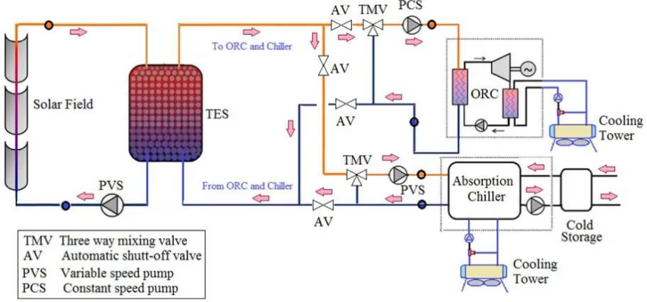
A schematic of the solar power plant using the organic rankine cycle for electric generation

and an absorption chiller for air conditioning purpose is shown in figure 1. The main purpose

from this plant is the scientific research and studying the performance of the plant. The main

parts of the plant are the solar collector field, storage tank, the organic rankine cycle, and

absorption chiller.

Fig. 1: Schematic diagram of the system.

2. Mathematical Modeling of the System

Mathematical modeling is a representation in mathematical terms of the behavior of real

devices and objects we want to know how to make or generate mathematical representations

or models, how to validate them, how to use them, and how and when their use is limited.

engineers and scientists have very practical reasons for doing mathematical modeling. In

addition, engineers, scientists, and mathematicians want to experience the sheer joy of

formulating and solving mathematical problems.

2.1. Organic Rankine Cycle Modeling

The organic Rankine cycle is consists of an evaporator, a condenser, a pump and a turbine.

From state 1 to 2, an ideal pump executes an adiabatic, reversible (isentropic) process to raise

the working fluid from the condenser pressure to the evaporator pressure. From state 2 to

state 3, an evaporator heats the fluid at a constant pressure (isobar transformation) moving

from a saturated liquid state 2’ to a saturated vapor state 3’ where all the liquid becomes

vapor. Then the fluid is superheated until it reaches the state 3. After, the superheat vapor

fluid enters in a turbine where it produces expansion through an adiabatic and reversible

process. The superheat process is necessary in order to guarantee that in the turbine only

vapor is present, this preserving the turbine blades from condensation and erosion. However,

the amount of superheat should be kept as low as possible in order to avoid waste of energy

and maximize the performance of the entire cycle. The typically used working fluid is an

organic fluid which is characterized by low latent heat and high density. These properties are

useful to increase the turbine inlet mass flow rate. Common working fluids that can be used

are R-123, R-134a and R-245fa. The properties of the working fluid have a significant impact

on the performance of the ORC cycle. The appropriate working fluids properties can lead to a

higher cycle performance.[7]

Modeling of the ORC is based on modeling of all components forming the cycle as shown in

figure 2. The evaporator and the condenser were treated as a heat exchanger. The turbine and

pump were simulated with isentropic process the components parameters were selecting for

Fig. 2: Schematic diagram of the storage tank with segments.[7]

One-dimensional heat transfer was assumed between the two heat transfer fluids. The thermal

oil represents the heating source fluid which flow in the evaporator as one phase flow, while

the organic fluid represents the cold fluid and pass through the evaporator in the different

three phases (liquid, two phase and vapor phase). So that, the evaporator was divided to three

main sections which are the liquid, two phase and the vapor sections each section was related

as a separated heat exchanger. As heat losses in heat exchangers are neglected, the amount of

the heat added to the working fluid in time is equal to the heat extracted from the heat source.

In general, for each zone the inlet temperature for the hot and the cold fluid stream are

and , respectively, and the outlet temperature for hot and cold streams are and ,

respectively. The outlet fluids temperatures were calculated from the following equation.[7]

……….. (1)

Where:

Q: The actual heat transfer rate (kW).

: The mass flow rates of the hot fluid (kg/s)

: The mass flow rates of the cold fluid (kg/s)

: The specific heat of the hot fluid (kJ/kg k)

: The specific heat of the hot fluid (kJ/kg k)

The working fluid heated in the evaporator to superheated vapor at constant pressure

(evaporating pressure). The heat transfer rate from the evaporator ( ) into the working fluid

….……… (2)

Where,

: is the mass flow rate of the working fluid (kg/s)

: is the enthalpy at points 3 and 2 (kJ/kg)

: is the Temperature degree at points 3 and 2 (K)

: is the specific heat of the working fluid (kJ/kg K)

The superheated vapor working fluid passes through the turbine to generate the mechanical

power. Firstly, we can calculate the enthalpy at point 4 from the following equation (Assume

Isentropic):

………. ……….… (3)

Where,

: is the turbine efficiency

: is the actual enthalpy at (kJ/kg)

: is the actual Temperature degree at (K)

: is the isentropic enthalpy at (kJ/kg)

: is the isentropic Temperature degree at (K)

Then, the power output from the ( ) turbine is given by:

…………..………... (4)

The exhaust vapor exits the turbine to the condenser where it is condensed by cooling water.

The heat rate removed by the condenser ( ) can be expressed as:

……… (5)

Where,

: is the enthalpy at point 1(kJ/kg)

: is the temperature at point 1 (K)

……….. (6)

To get the pump efficiency

………..…..………..……… (7)

Where:

: is the pressure at points 1 and 2 (kPa).

: is specific volume at point 1 (m3/kg).

Finally, the system efficiency is calculated as following:

……….………....… (8)

So, the gross electric power of the ORC unit is calculated as following

….………..…. (9)

Where

is the thermal power provided at the ORC unit evaporator from the storage tank.[9]

2.2. Thermal Absorption Chiller Modeling

With reference to the numbering system shown in figure 3, at point,[1] the solution is rich in

refrigerant and a pump,[2] forces the liquid through a heat exchanger to the generator.[3] The

temperature of the solution in the heat exchanger is increased. In the generator, thermal

energy is added and the refrigerant boils off the solution. The refrigerant vapor,[7] flows to the

condenser, where heat is rejected as the refrigerant condenses. The condensed liquid,[8] flows

through a flow restrictor to the evaporator.[9] In the evaporator, the heat from the load

evaporates the refrigerant, which flows back to the absorber.[10] A small portion of the

refrigerant leaves the evaporator as liquid spillover.[11] At the generator exit,[4] the fluid

consists of the absorbent–refrigerant solution, which is cooled in the heat exchanger. From

points,[6-1] the solution absorbs refrigerant vapor from the evaporator and rejects heat through

Fig. 3: Single effect, LiBr–water absorption cycle.[8]

To perform estimations of equipment sizing and performance evaluation of a single-effect

LiBr–water absorption cooler, basic assumptions and input values must be considered. With

reference to figure 3, the basic assumptions are

1. The steady state refrigerant is pure water.

2. There are no pressure changes except through the flow restrictors and the pump.

3. At points 1, 4, 8 and 11, there is only saturated liquid.

4. At point 10, there is only saturated vapor.

5. Flow restrictors are adiabatic.

6. The pump is isentropic.

7. There are no jacket heat losses.

Since, in the evaporator, the refrigerant is saturated water vapor and the temperature (T10) is

assumed, the saturation pressure at point 10 (P10), as calculated from curve fit, and the

enthalpy (h10). Since, at point 11, the refrigerant is saturated liquid; its enthalpy can be

calculated. The enthalpy at point 9 is determined from the throttling process applied to the

refrigerant flow restrictor, which yields that h9=h8. To determine h8, the pressure at this point

must be determined. Since, at point 4, the solution mass fraction x 4 is an input value and the

temperature at the saturated state was assumed, we can get the saturation pressure P4 and h4.

Considering that the pressure at point 4 is the same as in point 8; then h8 and h9 can be

Once the enthalpy values at all ports connected to the evaporator are known, mass and energy

balances can be applied to give the mass flow of the refrigerant and the evaporator heat

transfer rate.

He mass balance on the evaporator is:

………..……….. (10)

The energy balance on the evaporator is:

.……… (11)

Where:

: The mass flow rate at points 9, 10, and 11 (kg/s).

: The enthalpy at points 9, 10, and 11 (kJ/kg).

Since the evaporator output power and Liquid carryover from evaporator as a

percentage of were assumed, the mass flow rates can be calculated.

Since the values of and are known, mass balances around the absorber give:

………..………..(12)

And ……….……….. (13)

The mass fractions x1 and x6 are inputs, and therefore and (mass flow rate at points 1

and 6 respectively) can be calculated. The heat transfer rate in the absorber can be determined

from the enthalpy values at each of the connected state points. At point (1), the enthalpy (h1)

is determined from the input mass fraction x1 is an input value and the assumption that the

state is saturated liquid at the same pressure as the evaporator (P10). The enthalpy value at

point 6 (h6) is determined from the throttling model, which gives h6 = h5.

The enthalpy at point 5 is not known but can be determined from the energy balance on the

solution heat exchanger, assuming an adiabatic shell as follows:

………..……. (14)

Where:

The temperature at point 3 is an input value, and since the mass fraction for points 1 to 3 is

the same, the enthalpy at this point (h3) is determined. Actually, the state at point 3 may be

sub-cooled liquid. However, at the conditions of interest, the pressure has an insignificant

effect on the enthalpy of the sub-cooled liquid, and the saturated value at the same

temperature and mass fraction can be an adequate approximation. The enthalpy at point 2 is

determined from an isentropic pump model.

The minimum work input (w) can, therefore, be obtained from

………. ………..………. (15)

Where:

: is the pressure at points 1 and 2 (kPa).

: is specific volume at point 1 (m3 /kg).

It is assumed that the specific volume (v, m3/kg) of the liquid solution does not change

appreciably from point (1)-(2). The specific volume of the liquid solution can be obtained

from a curve fit.

Now, the unknown enthalpy value (h5) at point 5can be obtained from the equation of the

energy balance on the solution heat exchanger. The temperature at point 5 can also be

determined from the enthalpy value.

Finally, the energy balance on the absorber is

…….……….. (16)

The heat input to the generator is determined from the energy balance, which is:

………..……….………… (17)

The enthalpy at point 7 can be determined, since the temperature at this point is an input

value. In general, the state at point 7 will be superheated water vapor, and the enthalpy can be

determined once the pressure and temperature are known.

The condenser heat can be determined from an energy balance, which gives

……… (18)

……… (19)

3. RESULTS

After dividing the stored thermal power into ORC and TDC at different percentages, ORC

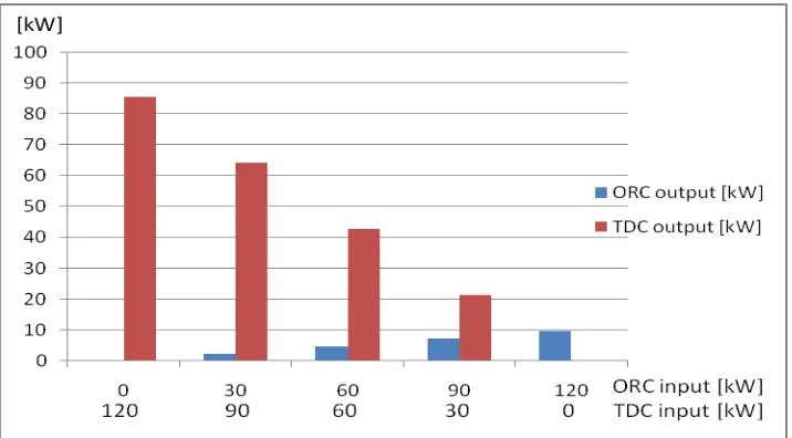
electric power (Wnet) and TDC cooling capacity ( ) are calculated. Figure 4 shows the

relation between the input thermal power of both ORC and TDC versus their outputs. With

the reference to this figure, it was noticed that both ORC net output power and TDC cooling

capacity increase with the increase of the input thermal power.

Fig. 4: ORC input thermal power vs. net output power and TDC input thermal power vs. cooling capacity.

3.1. Results of Organic Rankine Cycle

There are many parameters in the ORC which effect on the output electric power. Here, the

effect of inlet hot oil temperature and hot oil mass flow rate on the input thermal power, net

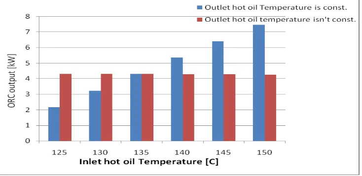
output power, and the ORC efficiency were investigated. Figure 5 shows the variation of

ORC electric power output, inlet thermal power, and ORC efficiency versus the inlet hot oil

temperature while the outlet hot oil temperature is/isn’t constant. As seen in this figure, when

Fig. 5: Inlet hot oil temperature vs. ORC net output power.

As shown in figure 5, it is observed that when the inlet hot oil temperature increases, net

electric power increases if the outlet hot oil temperature is constant and net electric power is

constant if the outlet hot oil temperature increases. This is because when the inlet hot oil

temperature increases and the outlet hot oil temperature is constant, the temperature

difference increases, thus increasing the input thermal power, which increases net electric

power. In the case of increasing the temperature of the outlet hot oil with the same increase in

the inlet hot oil temperature, the input thermal power is constant and this lead to that net

electric power is constant.

Figure 6 shows the effect of the mass flow rate of the hot oil (Msfo) on both the input thermal

power and net output power. From this figure, it is clear that increasing mass flow rate

increase both the input thermal power and net output power.

3.2. Results of Thermal Absorption Chiller

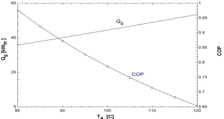
There are many parameters in the TDC modeling which effect on the COP like the effect of

generator and evaporator temperatures. Increasing input thermal power is definitely offset by

an increasing in the generator temperature. This statement is confirmed by figure 7 which

illustrates the effect of the generator temperature on both the input thermal power and

coefficient of performance.

Fig. 7: Generator temperature vs. input thermal power and COP (TDC).

As shown from figure 7, with the generator temperature increasing, the input thermal power

increases. This is because of in order to obtain a higher generator temperature; the input

thermal power must be increased. Also, when the generator temperature is increased, the

generator pressure is also increased, and this has the effect of lowering the COP of the unit,

considering that the pressures and temperatures at other points of the unit are kept constant.

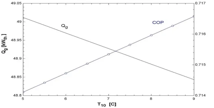
Figure 8 shows the effect of evaporator temperature on the required thermal power and the

coefficient of performance of the system. It can be seen that required thermal power

gradually decreases with the increase in evaporator temperature, thus increasing the

Fig. 8: Evaporator temperature vs. input thermal power and COP (TDC).

3.3. Analysis of kWh Cost

The study research plant cost is about 350,000 $. This cost is composed of about 140,000 $

for the solar field, 60,000 $ for the ORC, 30,000 $ for the chiller, and 120,000 $ for piping,

pumps, cooling towers, control, and other auxiliary equipment.

At each case study the cost of electrical kWh and refrigerant kWh are calculated as follow:

ORC capital cost ($) = 60,000

TDC capital cost ($) = 30,000

Solar Field capital cost ($) = 140,000

Pumping, control, and piping cost ($) = 120,000

Operation and Maintenance cost ($) “assumed” = 15,000 Plant life time (yr) “assumed” n = 25

Total thermal stored power (kW) = 120

ORC daily operation (hr) = 7

TDC daily operation (hr) = 7

The annual electrical power generated can be obtained as

kwhelec,y r = Wnet · ORChr · 365

. . . ………. (20)

The annual refrigerant kW generated can be obtained as

kwhref ,y r = Qe · TDChr · 365

The using percentage of the stored thermal power for both ORC and TDC as follow,

XORC =

Qadd 120

.. . . ………. (22)

XTDC = Q_g 120

.. . . ……… …. (23)

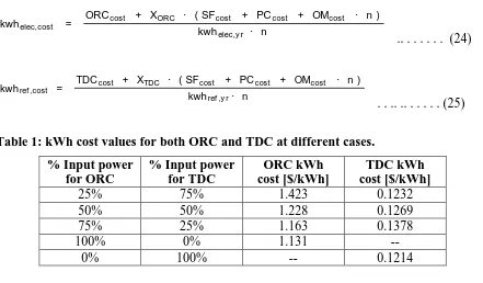
Finally, the cost of electrical kWh and refrigerant kWh can be obtained from eq. 24 and eq.

25.

kwhelec,cost =

ORCcost + XORC · ( SFcost + PCcost + OMcost · n )

kwhelec,y r · n

.. . . (24)

kwhref ,cost =

TDCcost + XTDC · ( SFcost + PCcost + OMcost · n )

kwhref ,y r · n

. . .. .. . . (25)

Table 1: kWh cost values for both ORC and TDC at different cases. % Input power

for ORC

% Input power for TDC

ORC kWh cost [$/kWh]

TDC kWh cost [$/kWh]

25% 75% 1.423 0.1232

50% 50% 1.228 0.1269

75% 25% 1.163 0.1378

100% 0% 1.131 --

0% 100% -- 0.1214

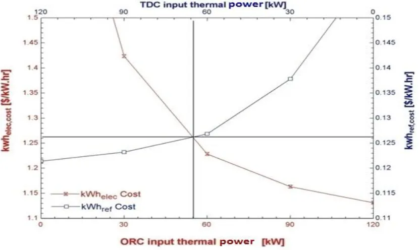
From Table 1, it was found that when increasing the input thermal power for both ORC and

TDC, the kWh cost decreases. Figure 9 shows the relation between the input thermal power

Fig. 9: Input thermal power vs. cost of kWh_elec. and cost of kWh_ref.

As shown in figure 9, the lowest price for ORC kWh is 1.131 $/kWh when 100% of the

stored thermal power is used by ORC to generate electricity. Also, the lowest price for TDC

kWh is 0.1214 $/kWh when 100% of the stored thermal power is directed to the TDC.

To compromise between both ORC and TDC, referring to figure 9, there is an intersection

point between the two curves that corresponds to the best operating condition when about

45.83% from the stored thermal power is used for ORC and about 54.17% is used for TDC.

In this case, the cost of electrical kWh from ORC is about 1.26$, while the cost of refrigerant

kWh from TDC is about 0.126$.

4. CONCLUSIONS

Referring to the analysis of the results after simulate the proposed research plant which

consists of solar collector field of 120 kW peak thermal capacity, thermal storage tank with 3

tons of therminol-66 oil, ORC of 8 kW nominal electric power production capacity, and TDC

of 35 kW cooling capacity. Both ORC net output power and TDC cooling capacity increase

with the increase of the input thermal power. When increasing the input thermal power for

both ORC and TDC, the kWh cost decreases. The lowest price for ORC kWh is 1.131 $/kWh

when 100% of the stored thermal power is used by ORC to generate electricity. Also, the

lowest price for TDC kWh is 0.1214 $/kWh when 100% of the stored thermal power is

To compromise between both ORC and TDC, The best operating condition is obtained when

about 45.83% from stored thermal power is used for ORC and 54.17% is used for TDC. In

this case, the cost of electrical kWh from ORC is about 1.26 $, while the cost of refrigerant

kWh from TDC is about 0.126 $.

REFERENCES

1. R. C. Bansal, T. S. Bhatti, and D. P. Kothari, “Bibliography on the application of

induction generators in nonconventional energy systems”, IEEE transactions on energy

conversion, 2003; 18(3).

2. L. Chang and H.M. Kojabadi, “Review of interconnection standards for distributed power

generation”, Large Engineering Systems Conference on Power Engineering (LESCOPE’

02), 2002; 36 - 40.

3. Umberto Desideri, PietroEliaCampana, “Analysis and comparison between a

concentrating solar and a photovoltaic power plant”, Applied Energy, 2014; 113:

422–433.

4. Wisam Abed Kattea Al-Maliki, Falah Alobaid, Vitali Kez, Bernd Epple, “Modeling and

dynamic simulation of a parabolic trough power plant”, Journal of Process Control, 2016;

39: 123–138.

5. Monica Borunda, O.A. Jaramillo, R. Dorantes, Alberto Reyes, “Organic Rankine Cycle

coupling with a Parabolic Trough Solar Power Plant for cogeneration and industrial

processes”, Renewable Energy, 2016; 86: 651-663.

6. Mustapha Merzouk, Nachida Kasbadji Merzouk, Said El Metenan, Omar Ketfi,

“Performance of a Single Effect Solar Absorption Cooling System (Libr-H2O)”, Energy

Procedia, 2015; 74: 130 – 138.

7. Mohamed H. Ahmed, Mohamed A. Rady and Amr M. A. Amin, “Multi Applications of

Small Scale Solar Power Plant Using Organic Rankine Cycle and Absorption Chiller”,

2014.

8. G.A. Florides, S.A. Kalogirou, S.A. Tassou, L.C. Wrobel, “Design and construction of a

LiBr–water absorption machine”, Energy Conversion and Management, 2003; 44:

2483–2508.

9. M. Astolfi, L. Xodo, M. C. Romano, E. Macchi, Technical and economic analysis ofa

10.Mohamed Rady, Amr Amin, Mohamed Ahmed, “Conceptual Design of Small Scale

Multi-Generation Concentrated Solar Plant for a Medical Center in Egypt”, Energy