(DOI: 10.24874/jsscm.2017.11.02.12)
Simulation of Fracture and Delamination in Layered Shells due to Blade
Cutting
F. Confalonieri1 and U. Perego1*
1Department of Civil and Environmental Engineering, Politecnico di Milano, Piazza Leonardo da Vinci, 32, Milano, Italy
e-mail: [email protected]; [email protected]
*corresponding author
Abstract
A new isotropic damage cohesive model for the simulation of mixed-mode delamination is presented. The model is based on consideration of the interface internal friction, naturally leading to coupled opening and shear damage mechanisms. Mixed-mode fracture energy turns out to be a direct outcome of the model and does not require the definition of an empirical law, additional to pure Mode I and II fracture energies. The model has been developed to account for delamination processes promoted by blade cutting of carton packages.
Keywords: Mixed-mode delamination, cohesive model, internal friction, isotropic damage.
1. Introduction
The finite element simulation of cutting and delamination in carton packages is a complex problem, involving several nonlinearities, each one requiring the development of ad hoc numerical tools. The adopted computational strategy for the simulation of cutting, based on the use of “directional cohesive elements”, has been described in (Pagani et al, 2015). This work will rather focus on the modelling of the delamination problem. Carton packages present a layered structure, consisting of paperboard, low-density polyethylene coatings, decor layers and possible layers of other materials, such as aluminum layers for food protection, so that delamination is a common failure mechanism, in particular in those regions where the cutting process is in progress. Although a large number of works devoted to the formulation of cohesive laws has been proposed in the literature, many of them are based on strong assumptions on the loading path and on the mixed-mode failure properties, or lack of thermodynamic consistency. Real-life delamination processes are indeed often characterized by mixed-mode loading conditions with varying mode ratio. Moreover, as demonstrated by several experimental works (see e.g. Benzeggagh and Kenane, 1996), the fracture energy significantly grows in passing from pure Mode I crack loading to pure Mode II.
in Section 3 to verify the consistency of the model under different loading paths. Finally, a numerical example is presented in Section 4.
2. Mixed-mode delamination model
The model, based on an isotropic damage formulation, is developed in a thermodynamic framework, which guarantees its consistency for any loading path. Let us introduce the free energy per unit surfacedefined as:
2
2
21 1 1
1 1
2 2 2
n n s
K d K d K
(1)
being dthe isotropic damage variable, K the elastic stiffness of the interface (assumed equal in pure Mode I and in pure Mode II crack loading conditions), n and sthe normal the shear opening displacements in the local reference frame. The Macauley brackets 〈 〉, denoting the negative and the positive part of the normal relative displacement, are introduced to account for the unilateral effect. The static variables of the model are defined by the following set of state equations:
1
1
n n n s s
t n K d K t s d K
(36)
2
21 1
2 2
n s
Y K K
d
(3)
where and represent the cohesive tractions in the normal and shear directions respectively, and Y is the strain energy released per unit growth of damage.
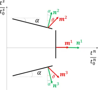
The interaction between normal and shear modes is governed by the definition of three damage modes, namely one opening- and two shear-dominated modes, in the plane of dimensionless cohesive tractions, as the ones shown in Fig. 1. Each damage mode is characterized by the normal unit vector ni. The inclination angle of the two shear-dominated
modes plays the role of a parameter of internal friction.
Fig. 1. Definition of damage mechanisms in tractions plane.
141 In order to account for the contribution of every damage mode to the overall decohesion process, let us introduce the effective cohesive stresses s s s , defined as the projection of the cohesive tractions onto the three normal vectors:
s Nt (4)
where N is a matrix gathering the components of the three normal unit vectors, while ̅ is the vector collecting the dimensionless cohesive tractions in the local reference frame:
1
1 0
2 sin cos
0 0 3 sin cos
T
n s
T t t
n s
t t n s
t t
n
t N n
n
(5)
being and the normal and the shear strengths in pure Mode I and II crack loading conditions. Writing eqn. (4) component-wise, one has:
1
2 sin cos 3 3 sin cos
n
s t
n s
s t t
n s
s t t
1 t n 2 t n t n
(6)
Similarly, the effective opening displacements, collected in the vector , can be defined as the projection of the dimensionless relative displacement onto a structural unit vector . In matrix form:
w Mδ (7)
where is a matrix gathering the structural unit vectors , while is the vector collecting the dimensionless opening displacements in the local reference frame:
1
0 2
sin cos
0 0 3 sin cos
T a
n s
T
n s b b
n s b b m
δ M m
m
(8)
being and the opening displacements at the onset of delamination in pure Mode I and II crack loading conditions, respectively, corresponding to and , and the angle defining the orientation of and ( is directed as for symmetry reasons). The constants and can be computed by imposing that the elastic strain energy is left unchanged, passing from the direct to the effective quantities, i.e.
1 1 1 1 2 2 3 3
2 2
T s w s w s w
t δ (9)
From eqn. (9), one obtains:
0 tan tan
0 00 0 0 0 2 cos cos
s s t
n s s
a t t b
(10)
142
1 tan tan
0 0 0 0
2 0 0 sin cos
2cos cos
3 3 0 0 sin cos
2cos cos
n n s s n
w t t
s s
t n s
w
s s
t n s
w 1 δ m 2 δ m δ m
(11)
Exploiting the definition of effective stresses and displacements, the overall elastic strain energy can be additively decomposed into the three contributions associated to the damage modes:
1 1 1 1 2 2 1 3 3 1
2 2 2 2
1 2 3
s w s w s w
T t δ
(12)
Defining the strain energy released per unit growth of damage associated to each mode is thus straightforward. Note that and :
1 1 2
1 tan tan
0 0 0 0 2
n n s s n
Y t t
d
(13)
2 1 2 2
2 tan tan tan tan
0 0 4
s s n s n s
Y t
d
(14)
3 1 2 2
3 tan tan tan tan
0 0 4
s s n s n s
Y t
d
(15)
Using eqns. (13), it easy to verify that , where is defined in eqn. (3). The angle is a parameter affecting the way the strain energy release rate is decomposed into its component. Henceforth, it will be assumed:
0 0 tan tan ,
0 0 n n t s s t
(16)
such that is always positive for any positive value of the normal opening displacement, under the condition α 45°. Note that, according to this decomposition, either or can attain negative values, though their sum is obviously always positive.
The damage activation function is written as a classical energy criterion:
1 2 3
2 3 1
1 1 2 2 3 3
0 0 0
k k k
Y Y Y
H Y H Y
d d d
(17)
1 2 3 1 2 3
1 2 3 1 2 3
1 2 3
1 2 3
n s
n s
d
d
Y Y Y n Y Y Y s
n n n s s s
Y Y Y Y Y Y
d d d
(18)
Finally, the following classical loading/unloading conditions hold:
0 d 0 d 0
(19)
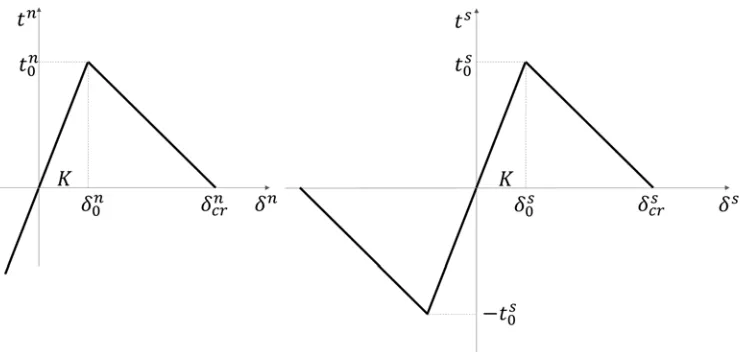
The shape of the cohesive law in the traction-opening displacement plane is governed by the internal variables . The case of a bilinear cohesive law is considered here. The use of any other functional form of the curve is also possible. For the bilinear law, it is possible to define the expression of as a function of the damage variable , such that a linear softening branch is obtained for pure Modes I and II crack loading (see Fig. 2).
Fig. 2. Pure Mode I and II cohesive laws.
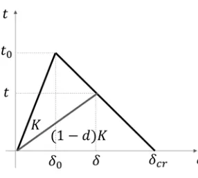
For the sake of simplicity, let us start from a 1D case, considering the bilinear law depicted in Fig. 3. The damage variable can be related to the current opening displacement by means of purely geometrical considerations, yielding:
0 0
0
cr cr
d
d
cr cr cr
Fig. 3. Bilinear cohesive law.
In the 1D case, the damage activation function reduces to:
1 ( ) 0 k Y d
(21)
being ̅ . At the onset of delamination ( → ̅ 1 , it holds that
0, 0 and 0 0, therefore the initial threshold is simply obtained as:
1 1 1
1
0 2 0 0 0 k Y Y t
(22)
while, in the softening phase:
2
1 1
1 0 0 0 0 0
2 2
0
k Y
Y t t
d
(23)
By substituting eqn. (18) into eqn. (21), we get the expression of as a function of the damage variable .
2
1 1
0 0 0 0
2 2 0 cr t t d cr cr
(24)
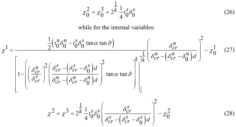
Applying the same steps to each of the two pure Modes, the expressions for the three initial thresholds and for the static-like variables can be obtained. Note that, because of the symmetry of the activation domain, one has and . In pure Mode II, 0, thus the Mode I dominated damage mode disappears from the damage activation function and and are independent of . In contrast, in pure Mode I and are not zero, because of the coupling between normal and shear openings: as a consequence, and depend both on and . The resulting expressions for the initial thresholds are:
1 1
1 tan tan
0 1 2 0 0 0 0
1 tan tan
n n s s
t t k k
145 1
1 2 3 2
0 0 k 4t0 0s s
(26)
while for the internal variables:
2 1 tan tan
0 0 0 0
1 2 1
0 1 0 2 2 0
1 tan tan
0
n n s s
t t n
cr
n n n d
cr cr
k k
s s s
n cr cr d
cr
s n n n d
cr cr cr
(27)
2 1
1
2 3 2 2
0 0 0
4
0
s
s s cr
k t
s s s d
cr cr
(28)
Using a classical argument, based on the Clausius-Duhem inequality for isothermal processes, it is possible to prove that the mechanical dissipation is always non-negative, being:
1 2 3 1 2 3 0
D Y d Y d Y d Y Y Y d Yd (29)
For the definition of its parameters ( , , , , , ), the proposed cohesive model requires the fracture energies and and the peak tractions and in pure Modes I and II crack loading conditions, in addition to the curve describing the evolution of fracture energy with the mode mixity ratio. All this information can be obtained by means of standard experimental tests, i.e. one Double Cantilever Beam (DCB) test for pure Mode I, one End Notch Flexure (ENF) test for pure Mode II and a set of Mixed Mode Bending (MMB) tests (Reeder and Crews 1992) for varying mode-mixity ratio.
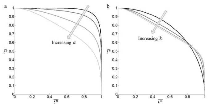
Fig. 4. a) Initial activation surface for 2 and for increasing values of the angle (namely 0°, 10°, 20° and 30°). b) Initial activation surface for 30° and for increasing values of the
exponent (namely 2,4,6,8).
3. Consistency tests
Three different tests proposed in the literature are here considered to prove the consistency of the cohesive model, also in case of non-trivial loading paths.
3.1. Radial path
Radial loading conditions with varying separation angles can be achieved by imposing
1 and , being an opening displacement linearly increasing from 0 to
0.05 and a coefficient describing the mode-mixity. Pure Mode I is recovered for 0, while pure Mode II corresponds to 1. The considered cohesive law properties for pure Mode I and II are reported in Table1.
K
6 MPa 6 MPa 0.1 N/mm 0.1 N/mm 1000 /
Table 1. Cohesive law properties in pure Mode I and II.
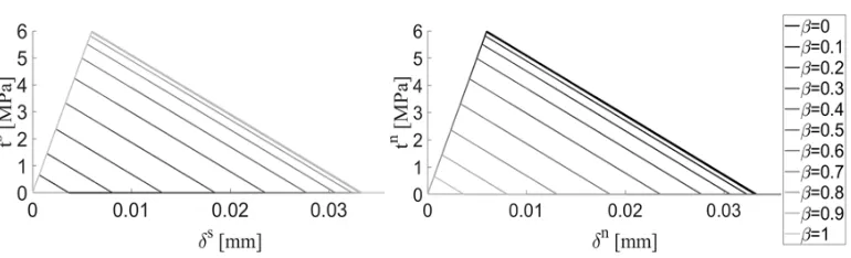
The traction-separation curves for increasing values of the mode-mixity ratio are plotted in Figure 5. As expected, under mixed-mode conditions, the curves in the plane
Fig. 5. Traction-separation curves for α 30° and 2.
3.2. Sinusoidal path
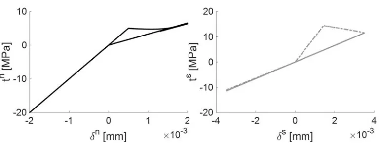
This consistency test has been proposed by Spring et al. (2016) to assess the consistency of the Park-Paulino-Roesler (PPR) cohesive model (Park et al, 2009) with respect to a mixed-mode loading/unloading condition. A sinusoidal history of opening displacements, displayed in Figure 6, is considered here by assuming that 2 ∙ 10 mm sin 0.15 and
10 mm3.5 sin 0.12 τ, being a time-like parameter. The cohesive properties defined by Spring et al. (2016) under pure Mode I and pure Mode II crack loading conditions are listed in Table 2.
K
40 MPa 15 MPa 0.1 N/mm 0.1 N/mm 10000 N/mm
Table 2. Cohesive properties in pure Mode I and II.
Fig. 6. History of applied normal and shear opening displacements.
Fig. 7. Traction-separation curves for 30° and 2, for sinusoidal path.
3.3. Non-proportional loading path
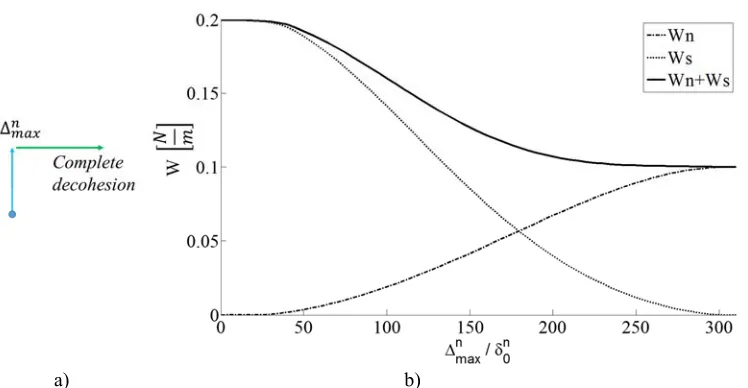
A non-proportional loading path, proposed by van den Bosch et al. (2006) and Park et al (2009) and depicted in Figure 8a, is considered here. The interface is loaded first in the normal direction up to ∆ and, then, in the shear direction up to failure, keeping the normal opening displacement constant. As in (van den Bosch et al. 2006) and (Park et al. 2009), consistency is tested in terms of the total work of separation, defined as:
max max
0 0
n n n s s s
W t d t d
n s
W W
(30)
Table 3 summarizes the considered cohesive properties: the pure Modes are characterized by different values of strengths and fracture energy.
K
6 MPa 12 MPa 0.1 N/mm 0.2 N/mm 10000 N/mm
Table 3. Cohesive properties in pure Mode I and II.
Figure 8b shows the works of separation computed for increasing values of max
n
, ranging froma) b)
Fig. 8. a) Non-proportional loading path. b) Work of separation computed for 30° and
4 .
4. Numerical example
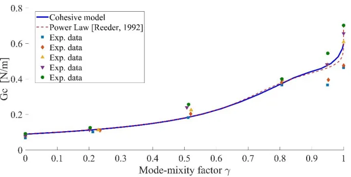
This numerical example assesses the capability of the proposed model to properly reproduce the mixed-mode behavior of a brittle epoxy resin (AS4/3501-6), experimentally tested through a set of MMB tests (Reeder and Crews, 1992) performed by Reeder (Reeder, 1993). The fracture energy is computed as the sum of the areas and beneath the normal and shear traction-separation curves, obtained with a series of radial paths with increasing mode-ratio. The adopted cohesive properties are: 0.09 N/mm, 0.6 N/mm,
150
Fig. 9. Experimental and simulated mixed-mode fracture energies ( 25°, k=12) for MMB test.
5. Conclusions
A new isotropic damage cohesive model has been proposed for the simulation of delamination under arbitrary, non-proportional mixed-mode loading conditions. The model is based on consideration of an internal friction dissipation mechanism, naturally resulting in a coupling between normal and shear damage modes. Tuning the internal friction parameter, it is possible to reproduce accurately the fracture energy under mixed-mode loading conditions, without introducing any empirical law to describe the variation of the fracture energy with the mode-mixity ratio. The model is thermodynamically consistent, as it implies rigorously positive dissipation, and exhibits a consistent mechanical response if used to simulate three widely employed consistency tests.
Acknowledgements The financial support of Tetra Pak Packaging Solutions is gratefully acknowledged.
References
Benzeggagh ML, Kenane M (1996). Measurement of mixed-mode delamination fracture toughness of unidirectional glass/epoxy composites with mixed-mode bending apparatus, Compos. Sci. and tech., 56, 439-449.
Pagani M, Perego U (2015). Explicit dynamics simulation of blade cutting of thin elastoplastic shells using “directional” cohesive elements in solid-shell finite element models. Computer Methods in Applied Mechanics and Engineering, 285, 515-541.
Park K, Paulino GH, Roesler JR (2009). A unified potential-based cohesive model of mixed-mode fracture. Journal of the Mechanics and Physics of Solids, 57, 891-908.
Reeder JR, Crews JH Jr (1992). Redesign of the mixed-mode bending delamination test to reduce nonlinear effects, J. Compos. Tech. Res., 14, 12–19.
151 Spring D, Giraldo-Londono O, Paulino GH (2016). A study on the thermodynamic consistency of the Park-Paulino-Roesler (PPR) cohesive fracture model. Mechanics Research Communications, 78, 100-109.