Theoretical description of functionality, applications, and limitations of SO 2cameras for the remote sensing of volcanic plumes

(1)

Atmos. Meas. Tech., 3, 733–749, 2010 www.atmos-meas-tech.net/3/733/2010/ doi:10.5194/amt-3-733-2010

Atmospheric

Measurement

Techniques

Theoretical description of functionality, applications, and

limitations of SO

2

cameras for the remote sensing of volcanic plumes

C. Kern, F. Kick, P. L ¨ubcke, L. Vogel, M. W¨ohrbach, and U. Platt

Institute for Environmental Physics, University of Heidelberg, Im Neuenheimer Feld 229, 69120 Heidelberg, Germany Received: 22 January 2010 – Published in Atmos. Meas. Tech. Discuss.: 12 February 2010

Revised: 25 May 2010 – Accepted: 2 June 2010 – Published: 29 June 2010

Abstract. The SO2camera is a novel device for the remote sensing of volcanic emissions using solar radiation scattered in the atmosphere as a light source for the measurements. The method is based on measuring the ultra-violet absorp-tion of SO2in a narrow wavelength window around 310 nm by employing a band-pass interference filter and a 2 dimen-sional UV-sensitive CCD detector. The effect of aerosol scat-tering can in part be compensated by additionally measuring the incident radiation around 325 nm, where the absorption of SO2is about 30 times weaker, thus rendering the method applicable to optically thin plumes. For plumes with high aerosol optical densities, collocation of an additional moder-ate resolution spectrometer is desirable to enable a correction of radiative transfer effects. The ability to deliver spatially resolved images of volcanic SO2distributions at a frame rate on the order of 1 Hz makes the SO2camera a very promis-ing technique for volcanic monitorpromis-ing and for studypromis-ing the dynamics of volcanic plumes in the atmosphere.

This study gives a theoretical basis for the pertinent as-pects of working with SO2 camera systems, including the measurement principle, instrument design, data evaluation and technical applicability. Several issues are identified that influence camera calibration and performance. For one, changes in the solar zenith angle lead to a variable light path length in the stratospheric ozone layer and therefore change the spectral distribution of scattered solar radiation incident at the Earth’s surface. The varying spectral illumi-nation causes a shift in the calibration of the SO2camera’s results. Secondly, the lack of spectral resolution inherent in the measurement technique leads to a non-linear relationship

Correspondence to: C. Kern ([email protected])

between measured weighted average optical density and the SO2column density. Thirdly, as is the case with all remote sensing techniques that use scattered solar radiation as a light source, the radiative transfer between the sun and the instru-ment is variable, with both “radiative dilution” as well as multiple scattering occurring. These effects can lead to both, over or underestimation of the SO2column density by more than an order of magnitude. As the accurate assessment of volcanic emissions depends on our ability to correct for these issues, recommendations for correcting the individual effects during data analysis are given.

Aside from the above mentioned intrinsic effects, the par-ticular technical design of the SO2camera can also greatly influence its performance, depending on the setup chosen. A general description of an instrument setup is given, and the advantages and disadvantages of certain specific instru-ment designs are discussed. Finally, several measureinstru-ment examples are shown and possibilities to combine SO2 cam-era measurements with other remote sensing techniques are explored.

1 Introduction

(2)

734 C. Kern et al.: Theoretical description of functionality, applications, and limitations of SO2cameras

and Mill´an, 1971; Stoiber et al., 1983), remote sensing tech-niques have become more and more established. More re-cently, the introduction of miniature ultra-violet spectrome-ters to the field (Galle et al., 2002; Edmonds et al., 2003) has reduced both the cost and complexity of such measure-ments, and applying the well-established retrieval techniques of differential optical absorption spectroscopy (DOAS) is now standard practice (Platt and Stutz, 2008). Aside from the obvious advantage of being able to measure volcanic emis-sions from a safe distance, it is also possible to implement measurement geometries that allow the retrieval of the total volcanic emission flux of a species, assuming lossless trans-port to the point of measurement (e.g. Galle et al., 2002, 2009; McGonigle et al., 2005).

The relatively high spectral resolution (typically below 1 nm) of the DOAS instruments allows the simultaneous re-trieval of different trace gas species. Aside from SO2, both BrO and NO2 have been detected in volcanic plumes in the past using scattered light DOAS observations (e.g. Bo-browski et al., 2003; Oppenheimer et al., 2005). Fourier transform infrared spectroscopy (FTIR) and active long-path DOAS can measure even more species in the IR and deep UV spectral ranges (Oppenheimer et al., 1998a; Burton et al., 2007; Kern et al., 2009), but they require more complex mea-surement geometries, as radiation at these wavelength ranges is not readily available in scattered sunlight.

The COSPEC and DOAS measurements allow determina-tion of the trace gas column density in a single direcdetermina-tion only, or rather in a typically small (of the order of 10−4steradian) element of solid angle, although at typically high sensitivity and (in the case of DOAS) high specificity. Obviously one-or two-dimensional (2-D) “images” of the plume are highly desirable for a variety of reasons (see below and Mori and Burton, 2006 and Bluth et al., 2007). First attempts to ob-tain 2-D trace gas images (of NO2, SO2and BrO) in the UV used the Imaging-DOAS (I-DOAS) approach (Lohberger et al., 2004; Bobrowski et al., 2006; Louban et al., 2009), where a column of image pixels is simultaneously recorded by an imaging spectrometer. A 2-D image is then constructed by scanning the viewing direction perpendicular to this column. While the I-DOAS technique appears to combine the advan-tages of DOAS with imaging capabilities, the price to be paid is a relatively long acquisition time (of the order of 15 min for a single image) and relatively complex setup of the in-strument. As the dynamic process governing the propagation and dispersal of volcanic plumes in the atmosphere occur on significantly shorter time scales (order of seconds), a simpler and faster means of recording 2-D images of volcanic gases is desirable.

The large amounts of SO2 present in volcanic plumes and the fact that SO2 is by far the most dominant absorber around 300 nm, however, make high spectral resolution mea-surements unnecessary for the quantification of SO2alone. Mori and Burton, 2006 and Bluth et al., 2007 have demon-strated the ability to measure 2-D SO2distributions in

vol-33 1

2

3

4

300 310 320 330 340

0.0 0.2 0.4 0.6 0.8 1.0

Re

la

ti

ve

f

ilt

e

r tr

a

n

smi

tta

n

c

e

Re

la

tive

sp

e

c

tr

a

l

in

te

n

s

it

y

Wavelength [nm]

T

A(λ)

I_S(λ)

0 2 4 6 8 10

σ(λ)

SO

2

a

b

sor

p

ti

on

cro

s

-se

ctio

n

[1

0

-1

9 cm 2 ]

5

6

Figure 1. Example of the spectral transmittance T(λ) of a band-pass filter which could be used 7

in a SO2 camera setup. In this case, the maximum transmittance is centered at 309 nm, a

8

region in which the SO2 absorption-cross-section σ(λ) is prominent (Bogumil et al., 2003).

9

Also shown in blue is an example spectrum of incident scattered solar radiation IS(λ), in this 10

case measured with an Ocean Optics©_{USB2000 spectrometer at 0.7 nm resolution.}

11

Fig. 1. Example of the spectral transmittanceT(λ) of a band-pass filter which could be used in a SO2camera setup. In this case, the

maximum transmittance is centered at 309 nm, a region in which the SO2absorption-cross-sectionσ(λ) is prominent (Bogumil et al.,

2003). Also shown in blue is an example spectrum of incident scat-tered solar radiationIS(λ), in this case measured with an Ocean Optics© USB2000 spectrometer at 0.7 nm resolution.

canic plumes using a simple UV-sensitive camera and band-pass filters only transmitting radiation at wavelengths signif-icantly influenced by SO2absorption. Here, this concept is first dealt with in a theoretical approach. Certain problems are identified, and methods for improving both the accuracy and technical implementation of the technique are described. Finally, some examples of the discussed methods and appli-cations are shown.

2 Measurement principle

In its simplest form, an SO2camera is solely composed of a UV sensitive camera and a single spectral band-pass fil-ter (referred to as filfil-ter A in the following) allowing only radiation in a narrow wavelength interval encompassing sig-nificant SO2 absorption structures to enter the camera op-tics. Figure 1 shows an example of the transmittance curve

TA(λ) of such a band-pass filter along with the absorption

cross-sectionσ(λ) of SO2. For each pixel, the intensity sig-nal collected through this filter is compared to a background intensity, either measured in a region in which no plume is present or interpolated from values acquired on either side of the plume.

In the absence of SO2, the wavelength-dependent light in-tensityI0,A(λ) arriving at each pixel of the 2-D camera CCD

is given by the intensity of scattered solar radiationIS(λ)

ar-riving at the instrument (see Fig. 1), the filter transmittance

TA(λ), and the quantum efficiencyQ(λ) of the detector.

(3)

C. Kern et al.: Theoretical description of functionality, applications, and limitations of SO2cameras 735

If SO2is present in the optical path of the incident radiation, the spectral intensity is attenuated according to the Beer-Lambert-Bouguer law.

IA(λ) = I0,A(λ)·exp(−σ (λ)·S(λ)) (2)

Here,σ(λ) is the absorption cross-section of SO2 andS(λ) is its column density, or the integral of the SO2 concentra-tion along the effective light pathL(ideally the line of sight through the plume).

S(λ) =

Z

L

c(x) dx (3)

Unfortunately, the effective light pathLcan deviate substan-tially from the line of sight through the plume. Especially in cases where volcanic plumes contain large amounts of SO2 or scattering aerosols or are viewed from a large distance, the effective light path may be significantly shorter or longer than a straight line through the area of interest. Radiation entering the field of view between the plume and the instru-ment (“radiative dilution”) shortens the effective light path, while multiple scattering inside the plume elongates it. In fact, the absorption of radiation by SO2in volcanic plumes is oftentimes sufficiently strong in itself to influence the effec-tive light path. Therefore, the column densitySis typically a function of the wavelengthλ. All of these effects were re-cently described and quantified by Kern et al. (2010), along with a suggested method for their correction using moderate resolution spectral data obtained from a DOAS instrument.

The negative logarithm ofI(λ)/I0(λ) gives the optical den-sityτ(λ), which is directly proportional to the SO2column densityS(λ) if SO2absorption is the only cause of light at-tenuation at the wavelengthλalong the effective optical path.

τ (λ) = −ln

_I

A(λ)

I0,A(λ)

= σ (λ)·S(λ) (4)

A spectroscopic instrument with sufficient resolution would measure the optical densityτ(λ) to retrieve the column den-sityS, but the SO2camera instead measures the integralIM,A

of the incident intensityIA(λ) over the transmission range

of the filter (the subscriptAdenotes intensities after having passed filterAas stated above).

IM,A =

Z

λ

IA(λ) dλ (5)

The respective relation is valid for the background measure-mentIN,A, although measuring this parameter can be

diffi-cult (see Sect. 2.2).

IN,A =

Z

λ

I0,A(λ) dλ (6)

From these measured quantities, the weighted average opti-cal densityτˆAis retrieved.

ˆ

τA = −ln

_I

M,A

IN,A

(7)

= ln IN,A

−ln

  Z

λ

I0,A(λ)·exp(−σ (λ)·S)·dλ

 

Using the notation defined in Eq. (1) and (2), the weighted average optical densityτˆAis given by

ˆ

τA = −ln



  R

λ

IS(λ)·TA(λ)·Q(λ)·exp(−σ (λ)·S(λ))·dλ

R

λ

IS(λ)·TA(λ)·Q(λ)·dλ



  (8) While the weighted average optical densityτˆAis obviously

a function of the SO2 column density S, it is important to note that the dependency ofτˆAonSis generally non-linear

(i.e.τˆA(S2) < (S2/S1)· ˆτA(S1)ifS1< S2). Only if the fil-ter wavelength transmittance range is sufficiently narrow that the SO2cross-sectionσ and the column densityScan be re-garded as independent of the wavelengthλin the measure-ment window can the integrated optical density be written as

ˆ

τA = −ln

IN,A·exp(−σ·S) IN,A

= σ·S = τ (9)

In this exceptional case, the weighted average optical den-sityτˆAwould be equal to the optical densityτ of SO2at the measurement wavelength and is therefore proportional to the column densityS. Then the instrument is in principle cali-bration free, as the relationship between the measured value

ˆ

τA and the column density S is defined by Eq. (9) (where σ(λ) is known from laboratory measurements).

In all other cases, Eq. (8) cannot easily be solved for the column densitySbecause the incident scattered solar radia-tion spectrumIS(λ), the filter spectral transmittanceTA(λ)

and the quantum yield of the detector Q(λ) are not well known. They must either be accurately measured (which is especially difficult forIS(λ), as it is constantly changing and

needs to be measured behind the plume) or an empirical in-strument calibration must be conducted to determine the re-lationship between the weighted average optical densityτˆA

(4)

736 C. Kern et al.: Theoretical description of functionality, applications, and limitations of SO2cameras 2.1 Normalized optical density/apparent absorbance

In general, the relationship between the measured weighted average optical densityτˆAand the column densitySof SO2is complex (see Eq. 8), but an empirical calibration can greatly simplify the data evaluation process. However, one condi-tion that must be fulfilled for the measurement principle de-scribed in Sect. 2 to remain valid is that the SO2 absorp-tion is the only parameter influencing light attenuaabsorp-tion in the transmitting wavelength window of the applied filterA. While this condition may approximately be fulfilled in the case of cloudless skies and translucent, aerosol-free (non-condensing) volcanic plumes (see Bluth et al., 2007; Mori and Burton, 2009), it will not generally be valid. In the presence of aerosols (water droplets or ash) in the volcanic plume, radiation entering the plume from behind will in part be scattered out of the instrument’s field of view, thus caus-ing a decrease in intensity. On the other hand, light entercaus-ing the plume from other angles will in part be scattered towards the instrument, thereby causing an increase in intensity. De-pending on the single scattering albedo of the plume aerosols, radiation will also be absorbed to some degree by the parti-cles. Finally, a species other than SO2 could be present in the plume and also absorb light in the measurement wave-length window. All of these processes compete with one another and can lead to attenuation or enhancement of ra-diation intensity being emitted from the plume towards the instrument when compared to the background sky intensity. If the measurement principle described in Sect. 2 is simply applied, each of these influences will distort the retrieved weighted average optical densityτˆA and therefore the SO2 column densityS.

Fortunately, in contrast to the SO2absorption, which is by far the strongest in the UV-wavelengths between about 250 and 320 nm (see Fig. 1 and Bogumil et al., 2003), aerosol scattering and absorption processes are of a broad-band na-ture, i.e. they are only weakly dependent on wavelength. Therefore, a second band-pass filter with a transmittance window above 320 nm, in the following referred to as fil-terB, can be used to quantify the amount of light attenua-tion (or enhancement) not originating from SO2absorption. Mori and Burton, 2006 successfully applied this technique at Sakurakima volcano in 2005. In this approach, band-pass filter A on the SO2 camera is at times replaced by filter

B. Both background (IN,B)and plume images (IM,B)are

recorded through filterB. Before the weighted average opti-cal densityτˆAis calculated, the ratio of pixel intensities

mea-sured through filterA(IM,A/IN,A)is normalized by the ratio

of pixel intensities measured through filterB (IM,B/IN,B).

Likewise, the weighted average optical densityτˆBcan be

cal-culated and subtracted from the optical densityτˆA. The thus

retrieved value is the normalized optical density τˆ,

some-times also referred to as the apparent absorbance AA.

ˆ

τ =AA= −ln

 

IM,A IN,A IM,B

IN,B

  = ln

 

IM,A IM,B IN,A

IN,B

  (10)

= ˆτA+ln

IM,B

IN,B

= ˆτA− ˆτB

Because of its greatly improved robustness in regard to the influence of scattering and broadband absorption effects, nor-malizing the optical density is necessary whenever a signifi-cant aerosol load is present or water condensation occurs in a volcanic plume.

Obviously, this approach assumes that the influence of aerosol scattering on the measured intensities is equal in both observed wavelength ranges. As typical ˚Angstrom expo-nents of volcanic aerosols lie between 0 and approximately 2 (e.g. Spinetti and Buongiornio, 2007), depending on their size distributions, the maximum error associated with this as-sumption is about 10%, and typical errors are around 5%. However, the radiative transfer between the sun and the in-strument can be dramatically changed by aerosols in the vol-canic plume, thus possibly changing the effective light path by 70% or more (Kern et al., 2010). This needs to be taken into account when calculating concentrations or fluxes from the measured optical densities. The condition that SO2must be the dominant narrow-band absorber in the filterA wave-length window remains a prerequisite for an accurate re-trieval of the SO2column densityS.

2.2 Obtaining the background intensity

The measurement principle of the SO2 camera is based on the ability to calculate the SO2column density S from the optical density τ (see Eq. 4). Due to the finite bandwidth of the applied interference filters, only a weighted average optical densityτˆA can be determined (Eq. 7). However, the

background intensityINat each pixel of the image is a also

needed for the retrieval. Obtaining this background image is often difficult, as an image of exactly the observed scene in absence of the volcanic plume is in principle required, as shown in Fig. 2.

Since this is usually impossible to obtain, one approach is to approximate the background intensityINby recording an

(5)

recorded at 90◦_{azimuth relative to this direction, simply} be-cause of the non-isotropic Rayleigh phase function.

A second approach to obtaining an appropriate back-ground image is to interpolate intensity values obtained on either side of the plume during the plume measurement. This method has the advantage that it is not necessary to pan the camera’s viewing direction. Considering the fact that a fre-quent recording of the background image is favorable be-cause it is influenced by solar zenith angle and aerosol/cloud conditions, this method is clearly advantageous. However, the technique also has a drawback: when using the first approach, a sophisticated flat-field correction is not neces-sary, as differences in radiation sensitivity across the detector (e.g. caused by optical vignetting, pixel quantum efficiency, and varying filter illumination angle, see Sect. 2.3) cancel out when calculating the normalized optical density according to Eq. 10. Only the detector offset and dark current, which can both easily be measured by taking dark images, need to be corrected. In this second approach, however, an accurate flat-field correction must be applied to any images before the background intensity can be interpolated from the pixels on either side of the plume. Therefore, it is necessary to care-fully characterize the relative sensitivity of each pixel on the detector. This can e.g. be achieved in the laboratory by mea-suring a homogeneously illuminated surface but is difficult to perform in the field.

2.3 Calibration issues

While the normalization of the integrated optical density is an important concept for the correction of broad-band light attenuation, the issue of how to derive the SO2column den-sity S from the observed optical density τˆ remains. Al-though it is in principle possible to construct a version of the SO2camera with inherent calibration by using very narrow band-pass filters (or possibly an interferometer), the trans-mittance window width would need to be on the order of 0.1 nm to ensure that the SO2 absorption cross-section can be assumed to be constant in the transmittance window (see Eq. 8). However, such a design greatly reduces the instru-ment light throughput and therefore the measureinstru-ment signal-to-noise ratio. For an optimal SO2sensitivity, the ideal band-pass filter transmittance T(λ) is considerably wider, as is shown in Sect. 3.2. In the past, calibration of the SO2camera has typically been conducted prior to or after measurements were made by inserting various SO2 calibration cells with known SO2 column densities S into the instrument’s field of view and determining an empirical relationship between the normalized optical densityτˆ(or apparent absorbance AA) and the SO2column densityS(see e.g. Dalton et al., 2009; Mori and Burton, 2009). Because the normalized optical densityτˆ depends on the incident scattered solar radiation spectrumIS(λ), the spectral transmittance of the band-pass

filtersT(λ),and the quantum efficiency of the detectorQ(λ) (see Eq. 8), this simple approach will only function properly

34 1

2

3

4

5

6

Figure 2. Schematic of the SO2 camera measurement geometry. The intensity of incident

7

radiation I(λ) is measured in and around the volcanic plume. In order to calculate the SO2

8

optical density τ(λ) from which the SO2 column density is derived, however, information

9

about the background intensity I0(λ) is needed (see Equation (4)). This information can be

10

difficult to obtain, especially if the illumination conditions behind the plume are 11

inhomogeneous e.g. due to the presence of clouds. 12

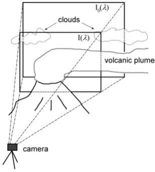
Fig. 2. Schematic of the SO2camera measurement geometry. The

intensity of incident radiationI (λ)is measured in and around the volcanic plume. In order to calculate the SO2optical densityτ(λ)

from which the SO2column density is derived, however,

informa-tion about the background intensity I0(λ)is needed (see Eq. 4).

This information can be difficult to obtain, especially if the illumi-nation conditions behind the plume are inhomogeneous e.g. due to the presence of clouds.

if all three parameters are constant in time. Unfortunately, this is usually not the case. While the quantum efficiency

Q(λ) can be assumed more or less constant in time and inde-pendent of wavelength in the region of interest, the other two parameters can vary depending on the measurement condi-tions and chosen optical setup.

In the following, a model was applied to study the sen-sitivity of the SO2 camera to variations in the spectral dis-tribution of the incident scattered solar radiation IS(λ) and

filter transmittanceT(λ). The transmittance of the band-pass filter Awas simulated using a Gaussian transmittance dis-tribution centered at λC = 309 nm and with a standard

de-viation of 3 nm (or FWHM of approximately 8 nm, shown in Fig. 1). This curve closely resembles the transmittance curve of the filter later chosen for the construction of the SO2 camera prototype (compare Fig. 9). For each wavelength be-tween 300 and 340 nm, the measured incident scattered solar radiation spectrumIS(λ) was multiplied by the filter

trans-mittanceTA(λ). The quantum efficiencyQ(λ) was not taken

into account further, as the quantum efficiency of the spec-trometer’s detector is intrinsically included in the measured solar spectrumIS(λ) and is thought to closely resemble that

of a typical SO2camera. In this manner, the spectral inten-sityI0,A(λ) was calculated according to Eq. (1). The

(6)

738 C. Kern et al.: Theoretical description of functionality, applications, and limitations of SO2cameras 35 1 2 3 4 5

300 310 320 330 340

0.0 0.2 0.4 0.6 0.8 1.0 In te n s it y [a rb . u n its] Wavelength [nm] IS(λ), 59° SZA

IS(λ), 70° SZA

IS(λ), 78° SZA

0 1 2 3 4 5 O 3 abs orpt ion c ros s -s e c tion [ 1 0 -19 cm 2 ]

O₃ cross-section

6

Figure 3. Measured spectra of scattered solar radiation IS(λ) for three different solar zenith 7

angles (SZA). While an absolute calibration was not achieved (the quantum yield Q(λ) of the 8

spectrometer is unknown), the intensity between 300 and 340 nm obviously increases relative 9

to the intensity at 340 nm with decreasing solar zenith angle. This is caused by a decrease in 10

optical path length of the detected radiation in the ozone layer. The ozone absorption cross-11

section (shown as dotted line) increases sharply towards lower wavelengths (Voigt et al., 12

2001, 223K). 13

Fig. 3. Measured spectra of scattered solar radiationIS(λ) for three different solar zenith angles (SZA). While an absolute calibration was not achieved (the quantum yieldQ(λ) of the spectrometer is un-known), the intensity between 300 and 340 nm obviously increases relative to the intensity at 340 nm with decreasing solar zenith angle. This is caused by a decrease in optical path length of the detected radiation in the ozone layer. The ozone absorption cross-section (shown as dotted line) increases sharply towards lower wavelengths (Voigt et al., 2001, 223 K).

2.3.1 Effect of the incident spectral intensity distribution

The spectrum of scattered radiation arriving at the earth’s surface depends on the solar zenith angle (SZA), especially in the UV wavelength region. For high solar zenith an-gles, the average optical path length through the stratospheric ozone layer is considerably longer than for lower SZAs.1As the ozone absorption cross-section increases dramatically to-wards deep UV wavelengths (see Fig. 3), the lower end of the scattered light spectrum is particularly influenced by these variations in optical path length.

In Figure 3, measurements of the incident scattered ra-diation spectrumIS(λ) made in Heidelberg, Germany on a

cloudless day are shown. Three spectra were recorded at 59, 70, and 78◦SZA, respectively. Each spectrum was normal-ized to its intensity at 340 nm. While all spectra fall off to null at approximately 300 nm, their relative intensities vary across the wavelength range from 300 to 340 nm, a result of variations in ozone optical density.

Using these measured spectra and the model described above, the effect of such variations on the weighted aver-age SO2 optical density τˆ measured with an SO2 camera can be discussed. In this first study, the spectral intensities

I0,A(λ) andIA(λ) were calculated using the incident

spec-tral intensities measured at the solar zenith angles 59◦ and 1_{There is one exception to this rule. For SZAs approaching 90}◦

the average optical path through the ozone layer decreases. This so-called Umkehr-Effect (G¨otz, 1931; G¨otz et al., 1934) is caused by an increase in the contribution of radiation scattered above the ozone layer to the total incident scattered light.

36 1 2 0.0 0.2 0.4 0.6 0.8 1.0

300 305 310 315 320 325

0.0 0.2 0.4 0.6 0.8 1.0

θ = 0° θ = 0°

Intens it y [ar b . uni ts

] I_0,A(λ)

I_A(λ) τ_Α = 0.0896 SZA = 59°

^ Intens it y [ar b . uni ts ] Wavelength [nm]

I_0,A(λ) I_A(λ) τ_Α = 0.0844 SZA = 78°

^

3

Figure 4. Modeled light intensity IA passing filter A of the UV-camera as a function of

4

wavelength λ for two different solar zenith angles (SZA). The blue curve (I0,A) assumes no

5

SO2 in the optical path (background spectrum), while the red curve (IA) represents an SO2

6

column density S of 400 ppmm. In both cases, light passes the filter in a perpendicular

7

direction (θ = 0). The ratio of integrated intensity under the background spectrum and under

8

the measurement spectrum yields the indicated integrated optical density τˆA according to

9

Equation (7). The two weighted average optical densities τˆA differ by 6%, even though the

10

assumed SO2 column density S was the same in both cases.

11

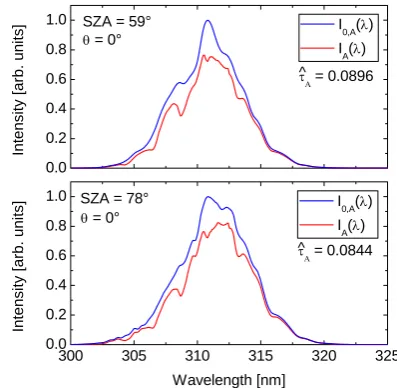
Fig. 4. Modeled light intensity IApassing filterAof the UV-camera as a function of wavelengthλfor two different solar zenith angles (SZA). The blue curve (I0,A)assumes no SO2in the optical path

(background spectrum), while the red curve (IA)represents an SO2

column densitySof 400 ppmm. In both cases, light passes the filter in a perpendicular direction (θ= 0). The ratio of integrated intensity under the background spectrum and under the measurement spec-trum yields the indicated integrated optical densityτˆAaccording to Eq. (7). The two weighted average optical densitiesτˆA differ by 6%, even though the assumed SO2column densitySwas the same

in both cases.

78◦. The four curves calculated in this manner are shown in Fig. 4. The presence of Fraunhofer absorption lines and, in the case ofIA(λ), superimposed SO2absorption lines makes for a highly variable spectral distribution which peaks around 311 nm even though the maximum filter transmission is lo-cated at 309 nm.

The SO2camera, however, does not measure the spectral intensitiesI(λ), but only the integrated intensitiesIM,A and IN,Adefined in Eq. (5 and 6). These can be calculated from

the distributions shown in Fig. 4 by integrating the spec-tral intensitiesI(λ) over the transmittance range of the fil-ter. Then, the weighted average optical density τˆA can be

calculated according to Eq. (7). The obtained values for the integrated optical densityτˆA are given below the legends in

Fig. 4. For the assumed measurement conditions, the two values differ by 6%. At higher solar zenith angles, the error will become even larger. This example therefore illustrates the fact that a correct calibration of the measured weighted average optical density τˆA will depend on the solar zenith

angle at the time of the measurement. In fact, a variation in the total stratospheric ozone column will have the same effect, as the total O3column density along the optical path determines the spectrumIS(λ). The use of a correction factor

(7)

37

290 300 310 320

0.00 0.05 0.10 0.15 0.20 Fil ter i llu min a tion an gle θ (°) Spec tr al t rans m itt anc e T A ( λ ) Wavelength [nm] 0 2 4 6 8 10 12 14 16 18 20 22 24 26 28 30 32 (a) 1

0 5 10 15 20 25 30

295 300 305 310 (b) Measured Equation (11) Cent ral t rans m is s ion wav e le ngth λc

Filter illumination angle θ 2

3

Figure 5. (a) Measured relative filter transmittance TA(λ) as a function of the illumination 4

angle θ. (b) Dots: measured central transmittance wavelength λc of the interference filter as a 5

function of filter illumination angle θ. Line: central transmittance wavelength according to 6

Equation (11) assuming a refractive index n of 1.6 (typical value for quartz optics). The filter 7

transmittance window shifts towards lower wavelengths if the filter is illuminated in a non-8

perpendicular direction (filter illumination angle θ≠ 0). 9

Fig. 5. (a) Measured relative filter transmittanceTA(λ) as a func-tion of the illuminafunc-tion angleθ. (b) Dots: measured central trans-mittance wavelengthλc of the interference filter as a function of filter illumination angleθ. Line: central transmittance wavelength according to Eq. (11) assuming a refractive indexnof 1.6 (typi-cal value for quartz optics). The filter transmittance window shifts towards lower wavelengths if the filter is illuminated in a non-perpendicular direction (filter illumination angleθ6=0).

2.3.2 The filter illumination angle

The central wavelengthλcof the transmittance window of a

band-pass interference filter decreases if the filter is not il-luminated perpendicularly (see e.g. Lissberger and Wilcock, 1959). For incidence anglesθbelow∼20◦, the central wave-lengthλc of the transmittance window can be approximated

by the expression

λc(θ ) ≈ λc(0◦)

s

1−sin 2_{(θ )}

n2 ≈ λc(0

◦₎ ₁₋ θ2 2n2

!

(11) wheren is the refractive index of the filter material. This relation was confirmed for the band-pass interference filters obtained for construction of the SO2camera prototype. Fig-ure 5 shows the measFig-ured relative transmittanceT(λ) of the filter as a function of the illumination angleθ. The trans-mittance window shifts towards lower wavelengths as the

il-38 1 2 3 4 0.0 0.2 0.4 0.6 0.8 1.0

300 305 310 315 320 325

0.0 0.2 0.4 0.6 0.8 1.0 ^

SZA = 59° SZA = 59°

θ = 10°

In

te

nsity [arb

. u

n

its] I0,A(λ)

IA(λ) τ_Α = 0.0977 θ = 6°

^ In te nsity [a rb . u n its] Wavelength [nm]

I_0,A(λ) IA(λ) τ_A = 0.1079

5

Figure 6. Modeled light intensity IA passing filter A of the SO2 camera as a function of

6

wavelength λ for two different illumination angles (θ = 6°and θ = 10°). The blue curve (I0,A)

7

assumes no SO2 in the optical path (background spectrum), while the red curve (IA) represents

8

an SO2 column density S of 400 ppmm. In both cases, the solar zenith angle (SZA) was kept

9

at 59°. The ratio of integrated intensity under the background spectrum and under the 10

measurement spectrum yields the indicated integrated optical density τˆA according to

11

Equation (7). The two integrated optical densities τˆA are 9% and 20% higher than for

12

perpendicular illumination (compare to Figure 4 (top)). 13

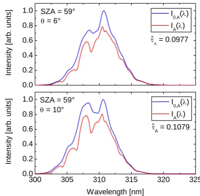
Fig. 6. Modeled light intensityIApassing filterAof the SO2

cam-era as a function of wavelengthλfor two different illumination an-gles (θ=6◦andθ=10◦). The blue curve (I0,A)assumes no SO2in

the optical path (background spectrum), while the red curve (IA) represents an SO2column densitySof 400 ppmm. In both cases,

the solar zenith angle (SZA) was kept at 59◦. The ratio of inte-grated intensity under the background spectrum and under the mea-surement spectrum yields the indicated integrated optical density

ˆ

τ_Aaccording to Eq. 7. The two integrated optical densitiesτˆ_Aare 9% and 20% higher than for perpendicular illumination (compare to Fig. 4, top).

lumination angleθincreases. Also, the maximum transmit-tance decreases and the transmission bandwidth of the filter increases slightly.

The dependence of the filter transmittanceT(λ) on the il-lumination angle can therefore change the sensitivity of the SO2camera to a certain SO2column density if the filter is not illuminated perpendicularly (θ= 0). This effect was studied using the model described in the previous section. Figure 6 depicts the modeled spectral light intensity passing filterA

of the SO2camera under the incidence anglesθ of 6◦(top) and 10◦(bottom). These angles correspond to a shift in the filter transmittance window of approximately 0.75 and 2 nm, respectively, towards shorter wavelengths (see Fig. 5), thus leading to a correspondingly larger influence of strong SO2 absorption bands (located around 300 nm, see Fig. 1) on the measured weighted average optical densityτˆA. This leads

(in our example) to an increase in the sensitivity of the SO2 camera (again, a constant column density of 400 ppmm was assumed). Compared to the weighted average optical density

ˆ

τA modeled for perpendicular illumination (Fig. 4, top), an

increase of 9% inτˆAwas obtained for an angle of incidence θ=6◦ and an increase of 20% in τˆA was found for θ=10◦.

(8)

39 1

2

3

4

Figure 7. Schematic of three different optical setups for SO2 cameras. In (a), the interference 5

filter is placed in front of the object lens. In this case, the filter illumination angle θ is a 6

function of the viewing direction and is largest close to the edge of the image. In (b), the filter 7

is positioned behind the objective. Here, a range of different angles θ are obtained for each 8

detector pixel. Inset (c) shows a setup designed to minimize θ. In linear approximation, the 9

maximum illumination angle is proportional to the ratio of the aperture size dA to the focal 10

length f1 of lens group 1 in this setup. 11

39 1

2

3

4

Figure 7. Schematic of three different optical setups for SO2 cameras. In (a), the interference

5

filter is placed in front of the object lens. In this case, the filter illumination angle θ is a

6

is positioned behind the objective. Here, a range of different angles θ are obtained for each

8

detector pixel. Inset (c) shows a setup designed to minimize θ. In linear approximation, the

9

maximum illumination angle is proportional to the ratio of the aperture size dA to the focal

10

length f1 of lens group 1 in this setup.

11 ₃₉

1

2

3

4

Figure 7. Schematic of three different optical setups for SO2 cameras. In (a), the interference 5

filter is placed in front of the object lens. In this case, the filter illumination angle θ is a 6

is positioned behind the objective. Here, a range of different angles θ are obtained for each 8

detector pixel. Inset (c) shows a setup designed to minimize θ. In linear approximation, the 9

maximum illumination angle is proportional to the ratio of the aperture size dA to the focal 10

length f1 of lens group 1 in this setup. 11

Fig. 7. Schematic of three different optical setups for SO2cameras.

In (a), the interference filter is placed in front of the object lens. In this case, the filter illumination angleθis a function of the viewing direction and is largest close to the edge of the image. In (b), the filter is positioned behind the objective. Here, a range of different anglesθare obtained for each detector pixel. Inset (c) shows a setup designed to minimizeθ. In linear approximation, the maximum illumination angle is proportional to the ratio of the aperture size

dAto the focal lengthf1of lens group 1 in this setup.

This significant change in sensitivity for non-perpendicular illumination can make a spatially inho-mogeneous calibration necessary if the angle of incidence on the filter is not equal for all measured radiation. In a simple setup of the SO2 camera, for example, the band-pass filter may be placed in front of the camera lens (e.g. .Mori and Burton, 2006). In this configuration (shown in Fig. 7a), light originating from different areas in the field of view will pass the filter under different angles. Therefore, the sensitivity (and the proper calibration) of the SO2camera will depend directly on the distancerd from the center of the image on

the detector. The angle of incidenceθon the filter is fixed for each pixel on the detector in this setup. This property can be used to make a first order correction for the incidence-angle effect. However, as discussed above, the correction not only depends on θ but also on other parameters, thus rendering an exact correction difficult. The maximum filter incidence angle θmax is equal to half of the camera’s total angle of viewα(see Fig. 7a).

A second design approach to the optics of an SO2camera is to mount the interference filters between the object lens and the detector. This setup is depicted in Fig. 7b. In this con-figuration, the filter incidence angleθ is no longer constant for each pixel on the detector. Instead, a range of different angles are realized, thus again leading to a pixel dependent effective transmission curve. On average, the incidence an-gleθis larger in this setup than if the filter is positioned in front of the lens, therefore causing a lower total transmission. However, as each pixel receives light from a range of angles,

and transmission is suppressed for large angles, the wave-length shift of the effective transmission curve is also less dependent on pixel position than in the initial setup (shown in Fig. 7a). Therefore, the sensitivity of the camera is less de-pendent on pixel position, although the total transmission is somewhat reduced towards the edge of the detector (for large

rd)thus causing vignetting.

Aside from the two simple setups which each use only a single camera lens, a number of other designs are possible. By using multiple lenses or lens groups, an optical system can be developed that minimizes the filter illumination angle. While it is impossible to discuss here all feasible alternatives, a few general remarks can be made. An ideal optical system will conserve radiance. The radianceB entering the system is a function of the total angle of viewα(B is proportional toα2)and the first aperture in the system dA (B is

propor-tional tod_A2). Once inside the system, the divergence of the light path can be decreased, but only by at the same time in-creasing the diameter of the apertures/optics (otherwise light is lost). Perfectly parallel propagation of light could only be achieved for optics infinitely large in diameter, or for an in-finitely small aperture at the front of the system. Therefore, designing an optical system with a perpendicular filter illu-mination angleθ for all incident light beams is impossible. A tradeoff between perpendicular filter illumination and op-tical throughput (defined by the aperture and lens size) will always need to be made. Keeping in mind that the shift ofλc

is approximately proportional toθ2for smallθ(see Eq. 11), very small angles of incidence are not required (wavelength shifts of less than 0.5 nm are obtained forθ <5◦, see Fig. 5b). One example of an optical system designed to minimize the filter illumination angle θ was developed for the SO2 camera prototype described in Sect. 3. It is shown in Fig. 7c. While a completely parallel filter illumination is not achieved, the optical design ensures that the range of re-alized illumination angles is constant for all viewing direc-tions, therefore yielding an identical effective filter transmis-sion curve for all pixels.

(9)

C. Kern et al.: Theoretical description of functionality, applications, and limitations of SO2cameras 741 2.3.3 Applying calibration corrections

Equation 8 can now be rewritten to include the effects dis-cussed above. The physical relation between the measured weighted average optical densityτˆAand the column density

of SO2is then given by

ˆ

τA= −ln



  R

λ

IS(λ,SZA)·TA(λ,θ )·Q(λ,β)·TO(r1..n)·exp(−σ (λ)·S(λ))·dλ

R

λ

IS(λ,SZA)·TA(λ,θ )·Q(λ,β)·TO(r1..n)·dλ





(12)

The spectrum of incident scattered radiation IS depends

on the solar zenith angle (SZA) and on the prevailing weather conditions (clouds and fog can significantly alter

IS). Therefore, the spectrum of incident solar radiation

typi-cally changes with time. In Sect. 2.3.2, it was shown that the transmission curve of the band pass filterTAdepends on the

illumination angleθ. If the effective transmission angle is not constant, this term will vary from pixel to pixel. In addi-tion, the quantum efficiency of each pixel may vary slightly depending on the angle of incidenceβ (see Fig. 7). Finally, the transmission of the optical systemTO will likely be a

function of the respective beam distancer from the center of the individual optical elements (vignetting caused by the individual apertures and/or the filter).

As Eq. (12) is likewise valid for calculating the weighted average optical densityτˆBin the long wave region, it

repre-sents a parameterization of the relationship between the SO2 column densitySand the measured normalized optical den-sity. It is evident that calibration of the SO2 camera is not trivial. In fact, due to the non-analytic integrals, the equa-tion cannot be solved forS. While, an empirical calibration can be performed by positioning calibration cells containing known amounts of SO2in front of the camera (see e.g. Dalton et al., 2009), it is important to keep in mind that the calibra-tion may depend on a number of pixel dependent parameters (e.g.θ,β,r1..n,rd depending on the applied optical setup)

and therefore must be performed individually for each pixel on the detector.

Also, Eq. (12) shows that the relation betweenτˆ andS

is non-linear. Whether or not a linear approximation is suffi-cient to describe the calibration of the instrument will depend on the variability and range of encountered values for each of the parameters in the equation, and especially the range of

S itself (see Dalton et al., 2009). Therefore, as many data points as possible should be collected for calibration, and these should span the entire range of measurement values.

Finally, the solar zenith angle is time dependent. There-fore, an empirical calibration using a gas cell will inevitably depend on the time of day. Fortunately, this effect is com-paratively small for the typical filter configuration modeled in Sect. 2.3.1, and is not likely to be a controlling error ef-fect for solar zenith angles smaller than 80◦in similar con-figurations. For measurements in the early morning or late evening, however, the influence of a change in the incident spectral intensity can be significant.

3 Design of an SO2camera prototype

Keeping the theoretical principles described above in mind, a prototype for an advanced SO2camera was constructed and tested in the field. Several components (optics, filters, detec-tor) were changed as compared to previous setups (Mori and Burton, 2006; Bluth et al., 2007) to improve the performance of the novel prototype.

3.1 Advanced optical system

An advanced optical system was designed specifically for the SO2camera in an attempt to reduce the illumination an-gle dependent calibration issues described in Sect. 2.3. A schematic of this design is shown in Fig. 7c. The optical system is composed of two lens groups between which the band-pass interference filter is located. An adjustable aper-ture is centered in the focal point of the first lens group. The total angle of view of the camera is therefore given by the relation

α=2·arctan

_R

eff

f1

≈2Reff

f1

(13) where Reff is the effective radius of the first lens (Reff =

R1−dA/2),f1is its focal length, anddAis the diameter of

the frontal aperture. Assuming the object of interest (e.g. the volcanic plume) to be at a large distance from the camera (compared to the focal lengths used in the optics), a virtual image of the viewed landscape is created in the opposite fo-cal plane of the first lens group. The band-pass interference filter is positioned behind this image so that dust or inhomo-geneities on the filter are not in focus. Behind the filter, a second group of lenses is used to project the virtual image onto the detector. The position of this lens group in relation to the detector and the virtual image can be varied such that the image is exactly scaled to fit the detector. If e.g. a 1 to 1 reproduction of the virtual image is wanted, the second lens group is placed at twice its focal lengthf2from the virtual image and the detector is likewise positioned at 2×f2from the lens group.

The great advantage of this setup over the simple setups discussed in Sect. 2.3.2 and shown in Fig. 7a and b is that the angle of incidenceθon the band pass filter no longer varies for individual pixel positions on the detector. Although a range of illumination angles is realized, this range is identi-cal for all pixels, thus leading to an identiidenti-cal effective filter transmission curve. The maximum angle of incidenceθmaxis controlled by the entrance aperturedAand the focal length of

the first lens groupf1, and can therefore easily be modified.

θmax =arctan

_d

A

2f1

≈ dA 2f1

(10)

angle θmax can only be achieved by reducing the radiance

B passing through the system. Reducing the aperture size

dA directly decreases light throughput (B ∼d_A2), and an

in-crease inf1results in a decrease in the total angle of viewα and thus also a quadratic reduction in radiance entering the system (B∼α2∼1/f₁2). For the prototype, a lens group with effective focal lengthf1of 25 mm was used and the aperture

d was typically set to 2.5 mm, resulting in a maximum illu-mination angleθmaxof less than 3◦, while the camera’s total angle of viewαwas approximately 20◦(the effective radius

Reffof the first lens was 5 mm).

Due to the relatively small aperture in the front of the opti-cal system, the accepted radianceB was considerably lower in this optical system than in prior setups (a typical entrance aperture for a simpler setup is 25 mm). However, by using a UV-sensitive back-illuminated CCD detector instead of a standard front-illuminated chip, the signal to noise ratio was sufficient to achieve a time resolution on the order of Hz. In fact, it was found that the main limitations to measurement time resolution are the camera’s digitization and readout time as well as the time required to exchange the band-pass filters, and not the exposure time itself.

3.2 Selection of the optimal band-pass filter

When selecting the band-pass interference filters for use in the SO2camera, several aspects must be considered. Both, the spectral position of the filter transmittance window as well as its width will determine the light throughput of the optical system. On the one hand, it can be advantageous to chose a very narrow-band transmittance window positioned directly on one of the strong SO2 absorption lines, as the SO2sensitivity will be high and the calibration becomes sim-pler (see Sect. 2, Eq. 8 and 9). On the other hand, the light throughput of such a system will be extremely low, thus re-sulting in an increased relative noise level. In the following, an attempt is made to determine the ideal filter transmittance width and central wavelengthλcfor filterA. FilterB is less

critical, as the incident solar radiation is much more intense above 320 nm and the instrument signal-to-noise is therefore decisively limited by filterA.

The model described in Sect. 2.3 was used to calculate the relative signal-to-noise ratio for a variety of filter configura-tions. The spectral transmittance curve of filterAwas again parameterized using a Gaussian distribution. For transmit-tance FWHM between 1 and 30 nm, the relative signal-to-noise ratio was calculated as a function of the central trans-mittance wavelengthλcof the filter. For the sake of

compara-bility, an identical maximum transmittance was assumed for all filters. This can only be considered an approximation, as very narrow band-pass interference filters tend to have lower maximum transmittances than wider filters, but actual trans-mittances vary, so this study may represent a somewhat opti-mistic estimate for narrow filters. Nevertheless, it gives some guidance on how to choose optimal filter parameters. When

40 1

2

3

4

5

300 305 310 315 320 325 0.0

0.2 0.4 0.6 0.8 1.0

Filter A central transmittance wavelength λ c [nm]

In

s

trum

ent

s

ignal-to-nois

e

rat

io [

a

rb.

unit

s

]

Filter A FWHM 1 nm 2 nm 5 nm 11 nm 15 nm 20 nm 30 nm

6

Figure 8. Modeled instrument signal to noise ratio as a function of the central wavelength of 7

filter A (for typical conditions, see text). Different colors represent different transmittance

8

window FWHM. A FWHM of less than about 2 nm is needed to resolve an individual SO2

9

line. However, the signal-to-noise ratio increases for larger FWHM up to a width of 11 nm 10

due to the increased light throughput. A further increase in the FHWM of the transmittance 11

curve degrades the signal-to-noise ratio as wavelengths are included where either no scattered 12

radiation is available or where SO2 exhibits only weak absorption. A broad optimum is found

13

for a bandwidth around 11 nm and a center wavelength λc of about 309 nm.

14

Fig. 8. Modeled instrument signal to noise ratio as a function of the central wavelength of filterA(for typical conditions, see text). Different colors represent different transmittance window FWHM. A FWHM of less than about 2 nm is needed to resolve an individ-ual SO2line. However, the signal-to-noise ratio increases for larger

FWHM up to a width of 11 nm due to the increased light through-put. A further increase in the FHWM of the transmittance curve de-grades the signal-to-noise ratio as wavelengths are included where either no scattered radiation is available or where SO₂exhibits only weak absorption. A broad optimum is found for a bandwidth around 11 nm and a center wavelengthλcof about 309 nm.

comparing filters with known transmittances, further normal-ization of the results given in Fig. 8 by the individual max-imum filter transmittances can easily be conducted. Also, a wavelength-independent detector quantum yield Qwas as-sumed. If the quantum yield of a specific detector changes significantly over the considered wavelength interval (300 to 325 nm), the quantum efficiency curveQ(λ) should be in-cluded in the model according to Eq. (8). Sensitivity studies showed that this can result in a slight shift in the ideal filter transmittance central wavelengthλc(see W¨ohrbach, 2008 for

details).

For the calculation of instrument signal-to-noise ratio (SNR), a second filter (filterB)was simulated using a trans-mittance window centered at λc = 325 nm and an

identi-cal FWHM as filter A. The normalized weighted aver-age SO2 optical densityτˆ was then retrieved according to Quations (8) and (10), assuming an SO2 column density of 4×1018molec/cm2, which is typical for volcanic plumes. Furthermore, as the noise of each measured integrated inten-sity is proportional to the square root of the inteninten-sity itself (photon statistics), the total noise of the weighted average optical density1τˆ could be quantified using Gaussian error propagation (see W¨ohrbach, 2008 for details). Dividingτˆby

1τˆyields a value proportional to the SNR.

(11)

41 1

2

3

4

5

300 310 320 330 340 0

2 4 6 8 10 12

SO

2 cross-section

Wavelength [nm]

SO

2

abso

rp

ti

o

n

cross-secti

on (10

-1

9 molec/cm 2 )

0.00 0.05 0.10 0.15 0.20

Filt

e

r t

ran

sm

it

tance

Filter A transmittance Filter B transmittance

6

Figure 9. Measured transmittance of the two band-pass filters used for construction of the SO2 7

camera prototype. Also shown (red) is the absorption cross-section of SO2 (Bogumil et al., 8

2003). 9

10

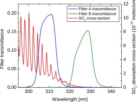
Fig. 9. Measured transmittance of the two band-pass filters used for construction of the SO2camera prototype. Also shown (red) is the

absorption cross-section of SO2(Bogumil et al., 2003).

due to strong ozone absorption, and the relative SNRτˆ/1τˆ drops. Towards longer wavelengths the incident intensity

IS(λ) increases, but the SO2 absorption cross-section be-comes smaller (see Fig. 1), therefore decreasing the mea-sured signal and thus also lowering the SNR.

Very narrow filters (less than 2 nm) are sensitive to individ-ual SO2absorption bands. For these, the calculated signal-to-noise ratio oscillates, depending on whether the transmit-tance window is on or between an SO2 absorption line. If a very narrow filter were to be used, the results indicate that placing the central wavelengthλc on the SO2 absorp-tion band at 311 nm would yield the highest SNR. Wider transmittance windows are no longer sensitive to individ-ual lines, but rather to the integral over several bands. As the filter transmittance width increases, the light throughput of the system increases thereby reducing the measurement noise and increasing the signal-to-noise ratio. However, if the transmittance window becomes too wide, parts of the so-lar scattered radiation spectrum are included in which SO2 absorption is less significant. Therefore, the measured signal no longer increases, and the signal-to-noise ratio decreases again.

The model indicates that the optimal filter transmittance curveT(λ) for band-pass filters used in an SO2 camera is centered atλc = 309 nm and has a FWHM of 11 nm.

How-ever, it should be noted that optical setups in which the filters are illuminated in a non-perpendicular direction will result in a shift of the effective filter transmission curve towards lower wavelengths. In such cases, the band-pass filter should be chosen such that the average effective transmission curve ex-hibits the optimal properties derived above. This may impli-cate using filters with longer maximum transmission wave-lengthsλc.

42 1

2

3

4

5

6

Figure 10. Schematic setup of the SO2 camera prototype. Light enters the instrument through

7

an aperture, passes through the band-pass filter and is focused on the CCD detector. The 8

measurement is controlled by an internal ITX PC, and data is saved on an internal hard drive. 9

The interface connectors are used to configure the measurement and collect data, as well as 10

for supply of 12V DC power. 11

Fig. 10. Schematic setup of the SO2camera prototype. Light enters

the instrument through an aperture, passes through the band-pass filter and is focused on the CCD detector. The measurement is con-trolled by an internal ITX PC, and data is saved on an internal hard drive. The interface connectors are used to configure the measure-ment and collect data, as well as for supply of 12 V DC power.

In our optical setup, the filter illumination angleθis neg-ligible, and the filters used for the construction of the SO2 camera prototype were chosen according to the results de-scribed above. Figure 9 shows the transmittances of the two band-pass interference filters acquired for this purpose from BK Interferenzoptik,© Nabburg, Germany. FilterAwas cen-tered at 309 nm, filterB at 326 nm. The spectral transmit-tance curvesT(λ) are slightly asymmetric, with FWHM of about 10 nm.

3.3 Technical implementation

A schematic of the designed SO2camera prototype is shown in Fig. 10. An ANDOR© 420 BU back-thinned CCD camera was chosen as a detector. This back thinned detector features a quantum efficiencyQthat is about 5 times higher at 300 nm than that of a standard front illuminated CCD (Q≈0.6). It has a wide image area of 26.6×6.7 mm (only about 11×6.7 mm were used) split into 1024×256 pixels, each with an area of 26 µm2and a well depth of 400 000 electrons. The camera is controlled by a Jetway© J7F21GE Mini-ITX PC via a PCI interface. The PC has a 1 GHz VIA© Eden processor, 1 GB RAM, and an 80 GB hard drive. It is powered off 12 V DC in-put voltage by an M1-ATX power supply system. The entire setup can alternatively be run off a 12 V DC power supply or a 12 V battery.

(12)

43 1

2 3 4 5 6 7

8

Figure 11. Visible image of Mt. Etna taken on October 15, 2007 from the town of Milo, 9

located approximately 11 km east-south-east of the volcano's summit. In this image, a dark, 10

ash-laden plume is being emitted from the new vent on the eastern flank of the south-east 11

crater. Plumes such as this one were intermittently emitted as a consequence of ongoing 12

explosions at this vent. 13

Fig. 11. Visible image of Mt. Etna taken on 15 October 2007 from the town of Milo, located approximately 11 km east-south-east of the volcano’s summit. In this image, a dark, ash-laden plume is being emitted from the new vent on the eastern flank of the south-east crater. Plumes such as this one were intermittently emitted as a consequence of ongoing explosions at this vent.

positioned in the optical path by a Trinamic Pandrive PD1-110-42-232 stepper motor driven by a motor controller con-nected to the serial port of the ITX PC.

4 Measurement examples

The designed SO2camera was tested in several measurement campaigns at Mt. Etna, Italy. Two interesting measurement examples will be discussed in this section. The first tests of the novel system were conducted in October of 2007. Vol-canic activity at Mt. Etna was elevated during the measure-ment period, with a new vent opening on the eastern flank of the active south-east crater. Periodically, explosions at this vent emitted short, ash-laden gas pulses. Figure 11 shows a visible image of such an explosive event ejecting a dark ash plume.

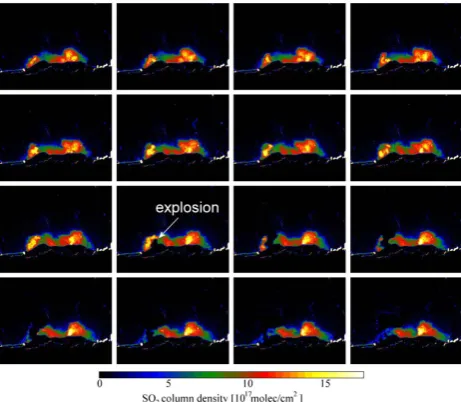
In the first test of the instrument conducted on 15 Octo-ber 2007, the SO2camera was used to measure the SO2 dis-tribution around the summit of Mt. Etna. Figure 12 shows an example time series of SO2images recorded from the town of Milo located about 11 km east-south-east of the volcano’s summit. The field of view of the SO2camera coincides with that shown in Fig. 11.

The first 9 images in Fig. 12 show the slightly variable distribution of SO2in the summit area of Mt. Etna. On this particular day, an easterly wind was blowing the volcanic plume away from the instrument. However, it is interest-ing to notice the elevated SO2column densities around both the north-east (typically the most active) and the south-east craters. This area of elevated SO2is not apparent in the visi-ble image (compare Fig. 11).

44 1

2

3

4

Figure 12. Time series of SO2 images recorded at Mt Etna on October 15, 2007 beginning at 5

13:00 local time. The time gap between each of the depicted images is 21 seconds. In the 10th 6

image, a dark cloud can be observed rising up from the vent on the eastern flank of the south-7

east crater. As UV-radiation cannot sufficiently penetrate this ash-rich plume, the signal from 8

the volcanic plume behind the ash cloud is blocked, resulting in an area of decreased SO2 9

column density. 10

Fig. 12. Time series of SO2images recorded at Mt. Etna on 15

Oc-tober 2007 beginning at 13:00 local time. The time gap between each of the depicted images is 21 s. In the 10th image, a dark cloud can be observed rising up from the vent on the eastern flank of the south-east crater. As UV-radiation cannot sufficiently penetrate this ash-rich plume, the signal from the volcanic plume behind the ash cloud is blocked, resulting in an area of decreased SO2column

density.

In the 10th frame shown in Fig. 12, an area of apparently reduced SO2can be observed on the southern side of the im-age. This area expands in the subsequently recorded images, and corresponds to a dark, ash-laden plume being emitted from the active vent on the eastern flank of the south-east crater (compare Fig. 11). Since UV-radiation can only partly penetrate this ash-rich plume, the enhanced signal from the volcanic plume behind the ash cloud is blocked. Therefore, the measured SO2column density drops to null for areas in which the ash cloud blocks the plume behind it. As the short pulse of ash-laden emissions dissipates, the original SO2 col-umn density can once again be measured.

(13)

45 1

2 3 4 5

6 7

Figure 13 – Visible (left) and SO2 camera (right) images recorded over the town of Milo at 8

the base of Mt. Etna on July 16, 2008. The rectangle in the visible image indicates the section 9

observed by the SO2 camera. The images were taken in southerly direction, the plume was 10

moving from right to left through the images. The SO2 image was slightly smoothed to 11

remove artifacts caused by dust in the optical system. A passive DOAS instrument was also 12

aimed at the volcanic plume. Its approximate viewing direction is indicated by a small 13

rectangular dot in both images. 14

Fig. 13. Visible (left) and SO2camera (right) images recorded over

the town of Milo at the base of Mt. Etna on 16 July 2008. The rectangle in the visible image indicates the section observed by the SO₂ camera. The images were taken in southerly direction, the plume was moving from right to left through the images. The SO2

image was slightly smoothed to remove artifacts caused by dust in the optical system. A passive DOAS instrument was also aimed at the volcanic plume. Its approximate viewing direction is indicated by a small rectangular dot in both images.

This is demonstrated in a second example. Here, a mea-surement conducted on 16 July 2008 at the same site in Milo is described. For this measurement, the SO2camera was not aimed at the volcano’s summit but in a southerly direction instead. On this particular day, a westerly wind was blow-ing the volcanic emissions towards the east, such that they passed above and to the south of Milo. In the left side of Fig. 13, a visible image of the volcanic plume is shown. The plume can be identified by the slight white haze apparent in the center of the image. The plume was blown from right to left through the image. A large black rectangle represents the field of view of the SO2 camera. On the right side of the image, an example SO2 distribution measured at 12:20 local time with the SO2 camera is shown. This image was smoothed slightly to remove artifacts caused by dust in the camera’s optical system. SO2column densities of more than 7×1017molec/cm2 (280 ppmm) were detected in the center of the plume.

Next to the SO2camera, a passive DOAS instrument (NO-VAC mark II, see Galle et al., 2009; Kern, 2009 for a com-plete description) was located on the same rooftop in Milo on 16 July 2008. For this measurement, the DOAS instru-ment was set to use a single, fixed viewing direction. The approximate location of this direction is given by the small rectangle in Fig. 13. However, the DOAS instrument’s field of view was 0.35◦which corresponds to an area of only ap-proximately 3×3 pixels on the SO2camera’s image.

As explained in Sect. 2, the lack of spectral resolution makes an empirical calibration of the SO2 camera neces-sary. This can be achieved using calibration cells containing known SO2concentrations, but maintaining a constant SO2 concentration can be difficult, as such cells tend to leak over time and, perhaps more importantly, the calibration depends on a number of time dependent parameters (see Sect. 2.3).

46 1

2 3 4 5 6 7

12:30 13:00 13:30 14:00 14:30 0

3 6 9

SO

2

c

o

lum

n

dens

it

y

[10

17 mo

le

c/cm

2 ]

SO

2-camera

DOAS

Time [local] 8

Figure 14 – SO2 column densities measured with the passive DOAS instrument compared to 9

those obtained in a small subsector of the SO2 camera’s field of view (after calibration with

10

the DOAS). The time series of the subsector with the best correlation to the DOAS data is 11

shown. 12

Fig. 14. SO2column densities measured with the passive DOAS

instrument compared to those obtained in a small subsector of the SO₂camera’s field of view (after calibration with the DOAS). The time series of the subsector with the best correlation to the DOAS data is shown.

DOAS, on the other hand, is intrinsically calibrated using lit-erature reference spectra. However, scanning DOAS instru-ments are limited to a single viewing direction, so a calibra-tion of the entire image of the SO2camera is not possible. Nevertheless, if a DOAS instrument is applied in parallel to measure SO2column densities in one point on the SO2 cam-era image, this point can be used for absolute calibration and the other pixels can be calibrated relative to this point.

This technique was applied in the measurements shown in Figs. 13 and 14. As the field of view of the DOAS instrument relative to that of the SO2camera was not accurately known, the SO2camera image was divided into a large number of subsectors and an SO2time series spanning two hours was extracted for each subsector using a rough calibration. The subsector with the best relative correlation to the time series from the DOAS instrument was then identified, and the cal-ibration was refined to match the intrinsic calcal-ibration of the DOAS. Finally, the calibration of the rest of the SO2 cam-era’s image was scaled to match the absolute calibration of the validated subsector. Calibrated in this way, the two time series showed a very good correlation, as is shown in Fig. 14. Remaining discrepancies are likely the effect of an imperfect match in field of view between the two measurements.

In this example, the advantages of calibrating the SO2 camera with a collocated DOAS instrument become appar-ent. Not only is the calibration performed intrinsically with the DOAS, the calibration can also be updated constantly, and even effects caused by variable radiative transfer that are only accessible through the high resolution spectral data ob-tained by the DOAS can be corrected.