www.the-cryosphere.net/7/1869/2013/ doi:10.5194/tc-7-1869-2013
© Author(s) 2013. CC Attribution 3.0 License.
The Cryosphere
A ten-year record of supraglacial lake evolution and rapid drainage
in West Greenland using an automated processing algorithm for
multispectral imagery
B. F. Morriss1, R. L. Hawley1, J. W. Chipman1, L. C. Andrews2, G. A. Catania2, M. J. Hoffman3, M. P. Lüthi4, and
T. A. Neumann5
1Dartmouth College, Hanover, New Hampshire, USA 2University of Texas, Austin, Texas, USA
3Los Alamos National Laboratory, Los Alamos, New Mexico, USA 4Swiss Federal Institute, Zürich, Switzerland
5NASA Goddard Space Flight Center, Green Belt, Maryland, USA
Correspondence to: B. F. Morriss ([email protected])
Received: 14 June 2013 – Published in The Cryosphere Discuss.: 18 July 2013
Revised: 7 November 2013 – Accepted: 8 November 2013 – Published: 12 December 2013
Abstract. The rapid drainage of supraglacial lakes
intro-duces large pulses of meltwater to the subglacial environ-ment and creates moulins, surface-to-bed conduits for future melt. Introduction of water to the subglacial system has been shown to affect ice flow, and modeling suggests that variabil-ity in water supply and delivery to the subsurface play an important role in the development of the subglacial hydro-logic system and its ability to enhance or mitigate ice flow. We developed a fully automated method for tracking meltwa-ter and rapid drainages in large (> 0.125 km2)perennial lakes and applied it to a 10 yr time series of ETM+and MODIS imagery of an outlet glacier flow band in West Greenland. Results indicate interannual variability in maximum cover-age and spatial evolution of total lake area. We identify 238 rapid drainage events, occurring most often at low (< 900 m) and middle (900–1200 m) elevations during periods of net filling or peak lake coverage. We observe a general progres-sion of both lake filling and draining from lower to higher elevations but note that the timing of filling onset, peak cov-erage, and dissipation are also variable. Lake coverage is sensitive to air temperature, and warm years exhibit greater variability in both coverage evolution and rapid drainage. Mid-elevation drainages in 2011 coincide with large surface velocity increases at nearby GPS sites, though the relation-ships between ice-shed-scale dynamics and meltwater input are still unclear.
1 Introduction
The Greenland Ice Sheet’s (GIS) contribution to sea level rise between 1993 and 2003 was estimated at
22 1
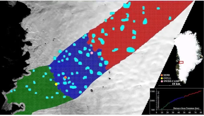
Figure 1. Study area in West Greenland, bounded by 69°48’N, 69°18’N, 50°23’W, and 2
48°0’W. 10 km swath on either side of the center flow band shown in green, blue, and 3
red, corresponding to <900 m, 900-1200 m, and >1200 m elevations—elevation profile 4
from GIMP 30 m DEM (Howat et al., in prep) inset, bottom-right. Chosen lake basins 5
shown in aquamarine (see Methods, 2.4). GPS stations at 33N0 and GULL (see Figure 6) 6
shown in orange and yellow, respectively. Air temperature data (3.3) collected at Swiss 7
Camp (pink). Background: ETM+ scene from August, 2002; Map Inset: MODIS true 8
color composite. 9
10
Fig. 1. Study area in West Greenland, bounded by 69◦480N, 69◦180N, 50◦230W, and 48◦00W. A 10 km swath on either side of the center flow band is shown in green, blue, and red, corresponding to < 900 m, 900–1200 m, and > 1200 m elevations – elevation profile from GIMP 30 m digital elevation model (Howat et al., 2012) inset (bottom right). Chosen lake basins are shown in aquamarine (see Methods, Sect. 2.4). GPS stations at 33N0 and GULL (see Fig. 6) are shown in orange and yellow, respectively. Air temperature data (3.3) were collected at Swiss Camp (pink). Background: ETM+scene from August, 2002; map inset: MODIS true color composite.
areas of thicker ice (> 1000 m ice thickness), moulins pro-duced by lake hydrofracture may be particularly important for meltwater transport because smaller moulins and cracks can no longer reach the bed (Van der Veen, 2007; Krawczyn-ski et al., 2009). Because of their ability to create conduits, provide large meltwater pulses, and potentially alter changes in the subglacial hydrologic system and ice flow, this study focuses on large supraglacial lakes and their drainages.
Past studies have used visible and near-infrared satel-lite imagery to identify and investigate the properties of supraglacial lakes using a variety of methods; however, many employ either manual lake identification (McMillan et al., 2007; Lampkin and Vanderberg, 2011) or automated lake identification using manually adjusted identification parame-ters for each image (Box and Ski, 2007; Sundal et al., 2009). These studies also require manual selection of cloud-free scenes and removal of false positives due to cloud shadows or other illumination anomalies. Two more recent studies (Selmes et al., 2011; Liang et al., 2012) take advantage of the contrast between lake water and the surrounding ice in MODIS band 1 (620–670 nm, red) to identify lakes and use automated methods for image selection and processing.
A fully automated processing algorithm is vital to this study because we aim to produce a ten-year surface cov-erage and drainage record, including analysis of over 100 Landsat 7 ETM+and over 8500 Aqua and Terra MODIS scenes over West Greenland. We automatically remove low-resolution and cloudy images and filter individual lake re-sults for localized cloud cover. We present the rere-sults from 802 lake maps of the study area – the number of useable scenesn (Fig. 4) ranged from 50 in 2002 to 109 in 2009,
with a mean of 73 MODIS and 7 ETM+scenes per year. Our results include both watered surface area and depth re-sults for the entire study area, but we choose to focus on 78 large (> 0.125 km2)lakes.
2 Methods
2.1 Study area
2.2 Imagery
Our study employs imagery from the Enhanced Thematic Mapper Plus (ETM+)aboard Landsat 7 and Moderate Res-olution Spectroradiometer (MODIS) on Aqua and Terra. The ETM+’s higher spatial resolution (30 m) provides a spatially detailed albeit temporally coarse record (16 day revisit pe-riod). While MODIS’s coarser spatial resolution (250 m in bands 1 and 2) limits reliable classification to lakes with ar-eas of ∼0.125 km2 (2 MODIS pixels) or larger, sub-daily satellite overpasses allow for much more sensitive analyses of temporal change. The detection algorithm uses red and near-infrared wavelengths, corresponding to ETM+ bands 3 (630–690 nm) and 4 (750–900 nm) and MODIS bands 1 (620–670 nm) and 2 (841–876 nm), respectively. We present results from images captured from 1 May to 30 September, annually, from 2002 to 2011. We exclude images with greater than 10 % study area cloud cover, determined from the auto-matic cloud cover assessment algorithm (Irish et al., 2006) for ETM+and the MOD/MYD35 Cloud Mask product for MODIS. We also limit analysis to MODIS scenes captured during midday (11:00–16:00 local time) where the study area is within 30◦ of nadir according to the MOD/MYD03 geolocation product to avoid issues with viewing geome-try and illumination. Because of their 2330 km-wide swath, MODIS 250 m resolution images exhibit effective resolu-tions as coarse as 750 m near the edges of each image. When analyzing relatively small, high contrast features such as lakes, this resolution degradation can result in misclassifi-cations. While small lakes (those nearer nominal resolution) may not be detected at all, the effective averaging that re-sults from this resolution loss can result in wide-scale water classification where none exists. Filtering those data that fall more than 30◦from nadir limits our analyses to those pixels with dimensions no greater than 333 m in the across-track direction and reduces the likelihood of misclassification.
2.3 Surface water identification
We convert ETM+and MODIS level 1 calibrated radiances to top-of-atmosphere (TOA) reflectances and reproject to the WGS-84 datum, UTM Zone 22. Surface water is identified based on a normalized difference lake index (NDLI), NDLI=
R r−Rnir
Rnir+Rr
, (1)
whereRrandRnirare the red (ETM+band 3, MODIS band 1) and near-infrared (ETM+ band 4, MODIS band 2) re-flectances of any pixel, respectively. Liquid water absorbs very highly in the near-infrared and can be used to delin-eate pooled water from the surrounding ice, which reflects highly in the infrared; however, degradation of the ice sur-face due to ablation and cryoconite concentration through-out the melt season drastically decreases infrared reflectivity resulting in overclassification of surface water. Because
wa-23 1
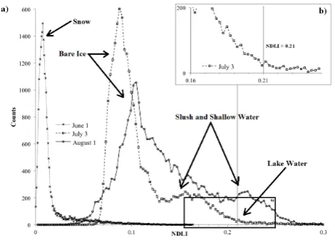
Figure 2. (a) NDLI histograms for select MODIS scenes from 2011. Dates chosen are 2
representative of pre-lake filling, mid season peak coverage, and late season, respectively 3
(see Figure 4). Vertical grey lines indicate identification threshold in (a) and in the mid 4
season zoom-in (b). 5
6
Fig. 2. (a) NDLI histograms for select MODIS scenes from 2011.
Dates chosen are representative of pre-lake filling, mid-season peak coverage, and late season, respectively (see Fig. 4). Vertical grey lines indicate identification threshold in (a) and in the mid-season close-up (b).
ter does not absorb as highly in the visible, the red bands are not as susceptible to this phenomenon, though they also exhibit less spectral separability between ice and water. To classify surface water accurately with either band alone re-quires a different threshold for each image. This normalized difference index better captures the differences between liq-uid water and the surrounding ice and allows us to use a sin-gle threshold value for all images analyzed. To determine a threshold, we examine the distribution of NDLI at different points during the melt season (Fig. 2). The three dates in Fig. 2 represent typical early, mid-, and late season cover-age states, respectively. NDLI gradually increases through-out the melt season as the surface transitions from snow to bare ice. Meltwater appears in the upper tail of the distribu-tion with NDLI increasing with water depth. To avoid mis-classifying shallow water and wet snow or ice as lake water, we place our threshold near the end of the distribution tail during peak coverage (Fig. 2b), when most of the standing water is in lake basins. We attribute the late season upward shift in the distribution to widespread shallow water and wet ice in the lower ablation zone that does not necessarily indi-cate an increase in lake volume. A threshold of NDLI=0.21 was used for all images. Adjusting the threshold by−10 % or
+10 % in all ETM+2011 images resulted in+9.3±3.7 % and−6.2±1.1 % change in coverage area, respectively.
2.4 Lake depth analyses
To determine lake depth and volume, we use a modified ver-sion of the method described by Sneed and Hamilton (2007). Lake depthzcan be determined by
z=ln A
d−R∞
Rr−R∞
whereAd is the lake-bed albedo or reflectance in the red band, R∞ the red reflectance of optically deep water, Rr the red reflectance of the lake pixel being analyzed, andg
a constant describing the optical properties of the lake water. AsR∞ requires optically deep (> 40 m; Sneed and
Hamil-ton, 2007) water, our estimation is limited to water in nearby fjords and Disko Bay, which may exhibit different scatter-ing and absorption coefficients than those described above. We takeR∞ to be the reflectance of a mid-bay pixel, free
of ice, sunglint, and outwash plumes and consistent in both ETM+and MODIS images from 3 July 2011 and use this value for all scenes (Sneed and Hamilton, 2011). While g
represents the characteristics of both upwelling and down-welling beam attenuation, Philpot (1989) estimates that g
can be related to the diffuse attenuation coefficient for down-welling light, Kd, as 1.5 Kd<g< 3Kd, with lower values coinciding with absorption-dominated water bodies, such as supraglacial lakes.Kdis calculated from the absorption,aw, and scattering, bm, coefficients for pure freshwater (Smith and Baker, 1981; Table 1),
Kd=aw+
bm
2 , (3)
at the appropriate sensor band wavelengths. We calibrate our estimate ofgusing field data from the lake near GULL (Fig. 1) by comparing the ETM+derived depth from 3 July 2011 during the lake’s filling phase to the measured depth from 28 July 2011 when the lake shore was at the same location during its gradual draining. We assume that the depths are equivalent within the resolution of the imagery. We use g=0.86 or 2.19Kd, appropriate for the relatively clear, absorption-dominated glacial meltwater.
To select the focus lake basins, we determined the max-imum depth for each pixel in the study area from ETM+
imagery between 2002 and 2011. Filtering out those areas with < 2 m maximum depths and, subsequently, those lakes with < 0.125 km2extent produced 78 distinct lakes (Fig. 1). To define our test basins, we include a 500 m radius buffer around each lake’s maximum extent and filter basin-full area measurements from our surface water inventory. Such mea-surements represent the coverage of each basin (and of entire regions of the ice sheet) by shallow water and wet ice and, because this occurs at low elevations and late in the season, generally do not coincide with the presence of lakes.
2.5 Drainage event identification
The rapid drainage of supraglacial lakes is a catastrophic oc-currence, resulting in the disappearance of the lake over a short time period. It is important to note that the time step between each image is not uniform, and because of this, as-sessing rapid drainage within any timing window is reliant on sufficient data density. While rapid drainage events can occur over a matter of hours (Das et al., 2008), we extend the identification window to 6 days to accommodate the
tempo-ral resolution of the coverage record and assume that slower drainages (through streams to moulins) occur on weekly to monthly timescales (field observation). Despite this conces-sion, image availability prevents reliable drainage detection during some time periods. To identify rapid drainage events, we compare local maxima in lake area,Lp, to subsequent lake areas,Ln, within a 6-day timing window. IfLnis more than 6 days after Lp, the window shifts until two points within a 6-day period can be compared. To qualify as a rapid drainage, a lake must lose critical area within a 6-day period; we define critical loss as 90 % of the year’s maximum area, (Lp−Ln)> 0.9Lmax. To prevent false positives, we require that the lake not refill within 6 days after the drainage. The drainage magnitude,Ld, is the lake area at the local peak,Lp, and the drainage time,td, is the midpoint between the time at local maximum,tp, and time of the critically low area,tn. We define the uncertainty in drainage time as the range between these values. This is summarized in Eq. (4):
if(Lp−Ln) >0.9Land(tn−tp) <6 days, (4) then rapid drainage ofLd=Lp occurred attd =
tp+tn
2 and uncertainty intdis bounded bytp andtn.
Rapid drainages that coincide with rapid filling in a nearby basin are automatically filtered from the drainage record be-cause they do not introduce water to the bed. Rapid drainage events are listed in the supplemental material.
2.6 Surface velocity from GPS
The ROGUE project maintains nine GPS (Trimble NetR7 with Trimble Zephyr Geodetic antennas) stations within the study area ranging in elevation from 650 to 1200 m. We present data from the two stations nearest the detected rapid drainage events in 2011. GPS positions were determined by carrier-phase differential processing relative to a bedrock-mounted base station using Track v.1.22 and final Interna-tional GNSS Service satellite orbits (methodology described in Hoffman et al., 2011).
3 Results and discussion
3.1 Volume vs. area (ETM+)
24 1
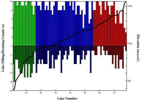
Figure 3. Lake filling and rapid draining occurence for individual lake basins. The total 2
number of years a lake filled appears as positive bar, colored according to its elevation 3
group (Figure 1). Total years where a rapid drainage event occurred appear as negative 4
bars. Lakes are sorted by increasing elevation which is plotted on the right y-axis as a 5
black line. Both lake and rapid drainage occurrence generally decrease with increasing 6
elevation; however, the largest high elevation lakes tend to drain rapidly, despite 7
increased ice thickness. 8
9
10 20 30 40 50 60 70
10 8 6 4 2 0 2 4 6 8 10
500 1000 1500
Lake Filling/Draining Counts (a)
Elevation (m.a.s.l.)
Lake Number
Fig. 3. Lake filling and rapid draining occurrence for individual
lake basins. The total number of years a lake filled appears as pos-itive bar, colored according to its elevation group (Fig. 1). Total years where a rapid drainage event occurred appear as negative bars. Lakes are sorted by increasing elevation, which is plotted on the rightyaxis as a black line. Both lake and rapid drainage oc-currence generally decrease with increasing elevation; however, the largest high-elevation lakes tend to drain rapidly, despite increased ice thickness.
D/zamong lakes, especially compared to variations in sur-face area (0.125 to 4.61 km2in the study area). When assess-ing all water within the study area, collectively, we find vol-ume to be highly correlated with surface area within our pre-defined lake basins (r2=0.896,n=167 361) and take lake area to be an appropriate proxy for volume. We find no sig-nificant correlation between volume and surface area when including out-of-basin waters (r2=0.443). We attribute the increased variance to widespread shallow standing water, which is particularly noticeable during the second half of the melt season at lower elevations (< 900 m) and can result in anomalously high surface area estimates that are not indica-tive of large volumes.
3.2 Surface water area inventory
Our water inventory includes surface area data from 730 MODIS and 72 ETM+scenes, tracks lake evolution through ten years, and identifies 238 rapid drainage events. Of the 78 lakes we tracked, 73 drain rapidly at least once during the study period, though many drain catastrophically in fewer than half the years they filled (Fig. 3). Both lake occur-rence and incidence of rapid drainage decrease with eleva-tion; while fewer full lakes afford fewer opportunities for rapid drainage, we attribute the decrease of rapid drainage with elevation to increased ice thickness – ice at our GULL boreholes (888 m a.s.l.) is over 700 m thick. Despite this, sev-eral of the highest elevation lakes drain catastrophically in the majority of years that they fill. While greater ice thick-ness poses a barrier to hydrofracture, it also produces larger
surface basins and greater lake areas and volumes. Above 1300 m a.s.l., increased lake size appears to overcome in-creased ice thickness, allowing lakes to create conduits to the ice sheet bed.
Results show high temporal variation in lake-filling onset (Fig. 4), ranging from mid-May (2010) to early July (2006). Lake filling occurs first at low elevations and proceeds up-ward, though in some years wide elevation ranges experience filling onset almost simultaneously. Lower elevations tend to lose lake area quickly, often before peak area has been reached in the other elevation bands. The middle elevation band (900–1200 m, blue in Fig. 1) hosts the most lakes and the highest potential area, but its lakes tend to be short-lived – the largest number of rapid drainage events occur in this elevation range. While there are fewer lake basins at high el-evation and those lakes fill during fewer years, high-elel-evation lakes can dominate coverage because of their large size, par-ticularly later in the season when low- and mid-elevation lakes have disappeared. Widespread high-elevation lake cov-erage is most prominent in 2004, 2007, and 2011, though notably few high-elevation rapid drainage events occur in these years (4, 4, 0, respectively). Maximum lake coverage ranges from 14.9 (2005) to 37.6 km2(2007), though this ac-counts for only 20–50 % of the maximum potential coverage (72.8 km2), calculated from the greatest extent of each lake in any given year. The large disparity between coverage and the maximum potential coverage is due not only to temporal and spatial variations in lake filling but also to variability in the mode and timing of lake drainage.
We observe large temporal variability in the timing of peak lake coverage and in coverage evolution. Rapid drainages occur most often during periods of net filling or near peak coverage, though neither the number of drainages nor their magnitude is closely related to coverage either lake by lake or regionally. Years with temporally narrow coverage peaks (2002, 2003, 2004, 2006, 2009, and, within the middle el-evation band, 2011) exhibit temporal clustering of rapid drainage events at a wide range of elevations around the cov-erage peak. While these rapid drainages contribute to the sub-sequent loss of lake coverage, they are accompanied by sig-nificant lake area lost to non-rapid, overland lake drainage in streams to moulins. In years without this temporal drainage clustering, lake coverage is lower in magnitude and more evenly distributed throughout the season (2005, 2008, 2010). In these years, rapid drainage events begin soon after filling onset in each elevation band and may prevent further lake filling.
3.3 Air temperature analyses
25 1
Figure 4. Evolution of total lake surface area (blue squares) for all valid ETM+ and 2
MODIS scenes (n) for each year of the study. Rapid drainage events (red circles) appear
3 0 10 20 30 40
Jun Jul Aug Sep
2.0 km2
1.0 0.50 0.25 d = 11 n = 50
2002
d = 29 n = 59
2003
d = 34 n = 90
2004
d = 22 n = 63
2005
Jun Jul Aug Sep
0 10 20 30 40
d = 24 n = 68
2006
Jun Jul Aug Sep
500 1000 1500
d = 16 n = 58
2007
d = 34 n = 90
2008
d = 22 n = 109
2009
d = 26 n = 65
2010
Jun Jul Aug Sep 500
1000 1500
d = 20 n = 76
2011
Total Lake Area (km
2)
Rapid Drainage Elevation (m.a.s.l.)
Fig. 4. Evolution of total lake surface area (blue squares) for all valid ETM+and MODIS scenes (n)for each year of the study. Rapid drainage events (red circles) appear at the affected lake’s elevation and are sized relative to magnitude (km2, see legend in 2002 panel) –d
represents the total number of drainages for any year. All plots share axes, detailed in 2002, 2006, 2007, and 2011.
the ready availability and reliability of AWS data and its cen-tralized location within the study area. We suggest that Swiss Camp sees the same synoptic forcing as the rest of the study area. Total lake area is sensitive to air temperature in the early season (Fig. 5); low-elevation lakes begin to form just prior to the onset of above-zero temperatures at Swiss Camp in each year, and prolonged periods of positive temperatures result in gains in total lake area. After the initiation of lake filling, the relationship between lake area and air temperature be-comes less clear. Many of the cooler years, those years with fewer than∼80 accumulated positive degree days, display a more convex distribution of positive degree days (PDDs), and peak lake coverage is coincident with the period of great-est PDD accumulation (Fig. 5a, b). In 2002, 2003, and 2009, total lake area decreases PDD accumulation slows and is not regained despite high temperatures at the end of the season. Rapid drainage events tend to cluster around peak coverage in these years. Warm years exhibit more of a linear to con-cave distribution of accumulated PDDs and much more
vari-able lake coverage and rapid drainage distributions. In 2010 when above-zero temperatures began in mid-May and per-sisted through September resulting in the highest observed total PDDs (167), total lake area remained at consistently low levels at all elevations throughout the season. This combina-tion of high PDDs and small total lake area also occurred in 2005, while the other two high PDD years (2007, 2011) exhibited extensive, prolonged lake coverage. In all but one case, warm temperatures after 1 August do not contribute to total lake coverage (GC-Net data were not available to in-vestigate the dual coverage peak in 2004), likely due to more efficient transfer of surface melt to the subsurface by existing streams and moulins.
3.4 Rapid lake drainage-induced ice flow
0 10 20 30 40
Jun Jul Aug Sep
2.0 km2 1.0 0.50 0.25
2003
Jun Jul Aug Sep
0 25 50 75 100 125 150
2009
Jun Jul Aug Sep
0 10 20 30 40
2010
Jun Jul Aug Sep 0
25 50 75 100 125
2011
Total Lake Area (km
2)
Cumulative PDD at Swiss Camp
Fig. 5. Total lake coverage (blue) and rapid drainage events (red circles, see inset scale) vs. cumulative positive degree day (PDD, grey)
from the GC-Net station at Swiss Camp for select years. Rapid drainage events are plotted at arbitrary vertical axis value to show temporal relationships. Lake filling begins just prior to PDD accumulation at Swiss Camp due to its higher elevation (1176 m) than the lowest lakes (369 m). Note the narrow coverage peaks and concentrated rapid drainage timing in low cumulative PDD years (2003, 2009). High PDD years may exhibit similar peak coverage and temporally localized drainage events (2011) or highly variable coverage and sporadic drainages (2010). Data from 29 July 2011 to 30 September 2011 are unavailable.
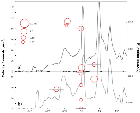
surface velocity record are unclear, though drainages appear to coincide with the three of the four major short-duration, mid-season speedups similar to those seen by Hoffman et al. (2011). Most noticeable is the clustering of drainage events around the 1 July surface velocity peak. The two largest drainages around the peak occurred within 10 m of 33N0’s (Fig. 6a) elevation, and that station recorded a larger surface positive velocity anomaly during the 1 July speedup than the station at GULL as well as a more pronounced slow-down following peak velocity (Fig. 6b). This slowslow-down is perhaps indicative of local reorganization of the subglacial hydrologic system following the nearby drainages, once the water supply begins to diminish. The final peak (11 July) may be the result of flow coupling associated with drainage out-side the study area or a rain event since we observe no coinci-dent rapid drainages; however, the number of usable images limits reliable drainage detection after 5 July.
4 Conclusions
We present a fully automated system for identifying and tracking supraglacial lakes in both ETM+and MODIS im-agery and use this system to track 78 large lakes along Ser-meq Avangnardleq between 2002 and 2011. We observe wide variations in filling onset and lake coverage evolution. While filling generally progresses inland and upward throughout the season, we observe interannual differences in filling on-set date in low-, mid-, and high-elevation zones of the study area ranging from a few days to over a month. Rapid drainage events are observed during all phases of filling but most of-ten near the seasonal coverage maximum or, in years with strongly elevation-staggered filling, near local peaks in lake
6/10 6/17 6/24 7/1 7/8 7/15 0
20 40 60 0 20 40 60 80 100 120
1000 1050 1100 1150 2.0 km2
1.0
0.50 0.25
Velocity Anomaly (ma
−1
)
Elevation (m.a.s.l.)
a)
b)
Fig. 6. Surface velocity data from 33N0 (a) and GULL (b) GPS
stations for summer 2011, smoothed to 36 h resolution and plot-ted as the velocity anomaly relative to the winter baseline at each site. Baseline (0) velocity anomaly (left vertical axis) is positioned at each GPS site’s elevation (right vertical axis). Rapid drainages appear as red circles (see inset scale), plotted at their elevation; horizontal grey bars represent temporal uncertainty (see Sect. 2.5). Black dots along the 33N0 baseline represent images used to define drainage events.
and ultimately on ice flow. Our air temperature analysis sug-gests greater variability in the evolution of lake coverage and rapid drainage events in warmer years. With the potential for widespread melt events as in July 2012 (Bennartz et al., 2012) and the continued progression of melt and lake forma-tion inland, monitoring surface water and further exploring its effects on the subsurface are vital in describing and pre-dicting the behavior of the Greenland ablation zone and the ice sheet as a whole.
Appendix A
Volume calculation parameters
λ 650 nm
Aλ 0.50
R∞,λ 2.0×10⁻²
g 0.868 m−1
Kd 0.397 m−1
Supplementary material related to this article is available online at http://www.the-cryosphere.net/7/ 1869/2013/tc-7-1869-2013-supplement.pdf.
Acknowledgements. This work was made possible by National
Science Foundation (NSF) grant NSF-OPP 0908156 awarded to R. L. Hawley. Special thanks to the National to Aeronautics and Space Administration (NASA) and Konrad Steffen’s group at the Coop-erative Institute for Research in Environmental Science (CIRES) for freely supplying imagery and climate data, respectively. Thanks also to CH2M Hill Polar Field Services and Air Greenland for logistical support in the field. Additional thanks are due to all those friends and colleagues who offered support and insight throughout the project.
Edited by: J. Stroeve
References
Bennartz, R., Shupe, M. D., Turner, D. D., Walden, V. P., Steffen, K., Cox, C. J., Kulie, M. S., Miller, N. B., and Pettersen, C.: July 2012 Greenland melt extent enhanced by low-level liquid clouds, Nature, 496, 83–86, 2012.
Box, J. E. and Ski, K.: Remote sounding of Greenland supraglacial melt lakes: implications for subglacial hydraulics, J. Glaciol. 53, 257–265, 2007.
Cazenave, A. and Llovel, W.: Contemporary Sea Level Rise, Ann. Rev. Mar. Sci., 2, 145–173, 2010.
Das, S. B., Joughin, I., Behn, M. D., Howat, I. M., King, M. A., Lizarralde, D., and Bhatia, M. P.: Fracture Propagation to the Base of the Greenland Ice Sheet During Supraglacial Drainage, Science, 320, 778–781, 2008.
Echelmeyer, K., Clarke, T., and Harrison, W.: Surficial glaciology of Jakobshavns Isbræ, West Greenland: Part I. Surface Morphology, J. Glaciol., 37, 368–382, 1991.
Hoffman, M. J., Catania, G. A., Neumann, T. A., Andrews, L. C., and Rumrill, J. A.: Links between acceleration, melting, and supraglacial lake drainage in the western Greenland Ice Sheet, J. Geophy. Res., 116, F04035, doi:10.1029/2010JF001934, 2011. Howat, I. M., Negrete, A., Scambos, T., and Haran, T.: A
high-resolution elevation model for the Greenland Ice Sheet from combined stereoscopic and photoclinometric data, Version 1.0, in preparation, 2013.
Irish, R. R, Barker, J. L., Goward, S. N., and Arvidson, T: Charac-terization of the Landsat-7 ETM+Automated Cloud-Cover As-sessment (ACCA) Algorithm, Photogramm. Eng. Rem. S., 72, 1179–1188, 2006.
Joughin, I., Das, S. B., King. M. A., Smith, B. E., Howat, I. M., and Moon, T.: Seasonal Speedup Along the Western Flank of the Greenland Ice Sheet, Science, 320, 781–783, 2008.
Krawczynski, M. J., Behn, M. D., Das, S. B., and Joughin, I.: Constraints on the lake volume required for hydro-fracture through ice sheets, Geophys. Res. Lett., 36, L10501, doi:10.1029/2008GL036765, 2009.
Lampkin, D. J. and Vanderberg, J.: A preliminary investigation of the influence of basal and surface topography on supraglacial lake distribution near Jakobshavn Isbræ, western Greenland, Hy-drol. Process., 25, 3347–3355, 2011.
Lemke, P., Ren, J., Alley, R. B., Allison, I., Carrasco, J., Flato, G., Fujii, Y., Kaser, G., Mote, P., Thomas, R. H., and Zhang, T.: 2007: Observations: Changes in Snow, Ice and Frozen Ground, in: Climate Change 2007: The Physical Science Basis. Contri-bution of Working Group I to the Fourth Assessment Report of the Intergovernmental Panel on Climate Change, edited by: Solomon, S., Qin, D., Manning, M., Chen, Z., Marquis, M., Av-eryt, K. B., Tignor, M., and Miller, H. L., Cambridge University Press, Cambridge, United Kingdom and New York, NY, USA, 2007.
Liang, Y., Colgan, W., Lv, Q., Steffen, K., Abdalati, W., Stroeve, J., Gallaher, D., and Bayou, N.: A decadal investigation of supraglacial lakes in West Greenland using a fully automatic detection and tracking algorithm, Remote Sens. Environ., 123, 127–138, 2012.
McMillan, M., Nienow, P., Shepherd, A., Benham, T., and Sole, A.: Seasonal evolution of supra-glacial lakes on the Greenland Ice Sheet, Earth Planet. Sc. Lett., 262, 484–492, 2007.
Philpot, W. D.: Bathymetric mapping with passive multispectral im-agery, Appl. Optics, 28, 1569–1577, 1989.
Price, S. F., Payne, A. J., Catania, G. A., and Neumann, T. A.: Seasonal Acceleration of inland ice via longitudinal coupling to marginal ice, J. Glaciol., 54, 213–219, 2008.
Schoof, C.: Ice-sheet acceleration driven by melt supply variability, Nature, 468, 803–806, 2010.
Selmes, N., Murray, T., and James, T. D.: Fast draining lakes on the Greenland Ice Sheet, Geophys. Res. Lett., 38, L15501, doi:10.1029/2011GL047872, 2011.
Smith, R. C. and Baker, K. S.: Optical Properties of the clearest natural waters (200–800 nm), Appl. Optics, 20, 177–184, 1981. Sneed, W. A. and Hamilton, G. S.: Evolution of melt pond volume
Sneed, W. A. and Hamilton, G. S.: Validation of a method for deter-mining the depth of glacial melt ponds using satellite imagery, Ann. Glaciol., 52, 15–22, doi:10.3189/172756411799096240, 2011.
Steffen, K., Box, J. E., and Abdalati, W.: Greenland Climate Net-work: GC-Net. CRREL 96-27 Special Report on Glaciers, Ice Sheets and Volcanoes, edited by: Colbeck, S. C., trib. to Meier, M., National Technical Information Service (NTIS), Springfield, VA, 98–103, 1996.
Sundal, A. V., Shepherd, A., Nienow, P., Hanna, E., Palmer, S., and Huybrechts, P.: Evolution of supra-glacial lakes across the Greenland Ice Sheet, Remote Sens. Environ., 113, 2164–2171, 2009.
Sundal, A. V., Shepherd, A., Nienow, P., Hanna, E., Palmer, S., and Huybrechts, P.: Melt-induced speed-up of Greenland ice sheet offset by efficient subglacial drainage, Nature, 469, 521–524, 2011.
Van den Broeke, M., Bamber, J., Ettema, J., Rignot, E., Schrama, E., Van de Berg, W. J., Van Meijgaard, E., Velicogna, I., and Wouters, B.: Partitioning Recent Greenland Mass Loss, Science, 326, 984–986, doi:10.1126/science.1178176, 2009.
Van der Veen, C.: Fracture propagation as a means of rapidly trans-ferring surface meltwater to the base of glaciers, Geophys. Res. Lett., 34, L01501, doi:10.1029/2006GL028385, 2007.