Open Access
Research
GOGOT: a method for the identification of differentially expressed
fragments from cDNA-AFLP data
Koji Kadota
1, Ryoko Araki
2, Yuji Nakai
1and Masumi Abe*
2Address: 1Graduate School of Agricultural and Life Sciences, The University of Tokyo, 1-1-1 Yayoi, Bunkyo-ku, Tokyo 113-8657, Japan and 2Transcriptome Research Center, National Institute of Radiological Sciences (NIRS), 9-1, Anagawa-4-chome, Chiba-shi 263-8555, Japan
Email: Koji Kadota - kadota@iu.a.u-tokyo.ac.jp; Ryoko Araki - a_ryo@nirs.go.jp; Yuji Nakai - yunakai@iu.a.u-tokyo.ac.jp; Masumi Abe* - abemasum@nirs.go.jp
* Corresponding author
Abstract
Background: One-dimensional (1-D) electrophoretic data obtained using the cDNA-AFLP method have attracted great interest for the identification of differentially expressed transcript-derived fragments (TDFs). However, high-throughput analysis of the cDNA-AFLP data is currently limited by the need for labor-intensive visual evaluation of multiple electropherograms. We would like to have high-throughput ways of identifying such TDFs.
Results: We describe a method, GOGOT, which automatically detects the differentially expressed TDFs in a set of time-course electropherograms. Analysis by GOGOT is conducted as follows: correction of fragment lengths of TDFs, alignment of identical TDFs across different electropherograms, normalization of peak heights, and identification of differentially expressed TDFs using a special statistic. The output of the analysis is a highly reduced list of differentially expressed TDFs. Visual evaluation confirmed that the peak alignment was performed perfectly for the TDFs by virtue of the correction of peak fragment lengths before alignment in step 1. The validity of the automated ranking of TDFs by the special statistic was confirmed by the visual evaluation of a third party.
Conclusion: GOGOT is useful for the automated detection of differentially expressed TDFs from cDNA-AFLP temporal electrophoretic data. The current algorithm may be applied to other electrophoretic data and temporal microarray data.
Background
Expression analysis based on comparison of one-dimen-sional (1-D) electrophoretic patterns is one of the few genome-wide approaches that don't require sequence information. There are a few methods such as differential display [1], amplified fragment length polymorphism (AFLP) [2], and its variants like cDNA-AFLP, an AFLP-derived technique for RNA fingerprinting [3]. The cDNA-AFLP method and related techniques such as HiCEP have
been widely used for gene discovery and monitoring tem-poral expression changes of transcript-derived fragments (TDFs) by comparing sets of time-course electrophero-grams [4-15]. However, inaccurate DNA fragment sizing often interferes with high-throughput analysis.
A major source of incorrect estimation of fragment lengths is the use of wrong size marker peaks when the true peaks are masked by intense peaks nearby [12,16]. Such electro-Published: 30 May 2007
Algorithms for Molecular Biology 2007, 2:5 doi:10.1186/1748-7188-2-5
Received: 6 February 2007 Accepted: 30 May 2007
This article is available from: http://www.almob.org/content/2/1/5
© 2007 Kadota et al; licensee BioMed Central Ltd.
pherograms are locally expanded or compressed and the deviation from the true electropherogram reaches a maxi-mum around the length of the wrong marker peak. Although a previous normalization strategy for HiCEP (a cDNA-AFLP-based expression profiling technique) data analysis [12] can correct this kind of inappropriate frag-ment sizing, slight variations in the lengths of identical TDFs across different electropherograms still remain. Even if the variations of individual TDFs across electrophero-grams are very small (e.g., within 1 bp), cumulative errors of fragment sizing interfere with accurate alignment of identical TDFs and make visual evaluation troublesome. Therefore, the minimization of variations of identical TDFs is a prerequisite for accurate alignment and easy vis-ual evaluation.
The purpose of the present study is the identification of differentially expressed TDFs from HiCEP time-course data using a method (called "GOGOT") proposed here. This is essentially the purpose of microarray analysis. However, the bottleneck is the construction of an expres-sion matrix of TDFs (rows) per time points (columns) of HiCEP electrophoretic data due to the problem of imper-fect alignment, though most microarray analysis uses such matrices as given data (e.g., [17,18]). GOGOT constructs an expression matrix consisting of valid TDFs whose alignment accuracies are objectively high and ranks TDFs according to their degrees of differential expression using a special statistic. The performance of GOGOT is demon-strated by analyzing a large set of HiCEP time-course data obtained from mouse embryonic stem (ES) cells.
Results and discussion
A total of 256 primer combinations (16 MspI-NN primers combined with 16 NN-MseI primers; N = {A, C, G, T}) of HiCEP time-course data (mouse embryonic stem cells at 0, 12, 24, 48, and 96 h after adding stimulation for differ-entiation) was analyzed. HiCEP samples were technically duplicated and thus designated as 0h-1, 0h-2, 12h-1, 12h-2, 24h-1, 24h-2, 48h-1, 48h-2, 96h-1, and 96h-2. The data were preprocessed by a method which corrects fragment sizing errors caused by the mis-selection of size marker peaks [12].
The remaining slight variations in the lengths of subjec-tively identical TDFs across different electropherograms would be sufficient to make visual evaluation tedious and tends to cause imperfect alignment of the same peaks across different electropherograms (such as shown in Fig. 1a). In this work, we applied the current method to each of the 256 sets (primer combinations).
To both improve the alignment and make visual evalua-tion less difficult, we adopted a method (called GOGOT) for the HiCEP expression analysis. Briefly, the procedure
consists of four steps: (1) normalization of peak fragment lengths, (2) peak alignment, (3) normalization of peak heights, and (4) identification of differentially expressed TDFs. In our experience, step 1 is peculiarly important for easy visual evaluation, especially when the number of electropherograms being compared is increased, regard-less of successful or unsuccessful peak alignment [12,19].
In this paper, peak alignment for HiCEP electrophoretic data (Step 2) is performed using an algorithm based on complete linkage hierarchical clustering [20], though algorithms based on dynamic programming (DP) have widely been used for the purpose [21-25]. Perhaps a sophisticated DP-based method could perform accurate alignment such as shown in Fig. 2 for electropherograms in Fig. 1 without step 1. Nevertheless, the results of peak alignment for normalized electropherograms such as shown in Fig. 2 obtained from our two-step process (step Typical example of HiCEP electropherograms before nor-malization of peak fragment lengths by GOGOTnormL
Figure 1
1 and 2) were satisfactory and those visual evaluations were very easy. The advantageous characteristics of our two-step approach over conventional DP-based methods [21-25] may be (i) easy visual evaluation by virtue of step 1 and (ii) easy traceability of why peaks are merged into a single TDF by virtue of a simple clustering-based method at step 2 (for details, see Methods). In general, labor-intensive visual evaluation of the electropherograms imposes bottlenecks on high-throughput expression anal-ysis by electrophoretic methods including cDNA-AFLP [23]. Although there is currently no convincing rationale for choosing between the different methods, our two-step approach may eventually increase throughput. We dem-onstrate the feasibility of GOGOT in the rest of this sec-tion.
Normalization of peak fragment lengths and its effect to peak alignment (Step 1 and 2)
Let be the ith TDF (i = 1,..., n
k) in electropherogram Pk
(k = 1,..., m; in this case m = 10). A TDF F is characterized by its length L (in bp), peak height H, and area A (in arbi-trary units). The input data can be represented as 256 sets of (Li, Hi, Ai)k. Each electropherogram can be
approxi-mated by a Gaussian kernel using the input data [21-24]. The approximate electropherogram P(t), which is com-posed of n fragments Fi (i = 1,..., n), at length t (in bp) is given by
, where σi =
Ai/(Hi ), the standard deviation of a Gaussian curve
approximated to the shape of the Fi.
As demonstrated in Fig. 1a, the direct application of clus-tering-based peak alignment (step 2) to HiCEP electro-phoretic data does not work well because of the variation in the lengths of subjectively identical TDFs across electro-pherograms. In our opinion the four peaks aligned with black bold lines do not originate from identical TDFs and should be merged into the neighboring TDFs so that the peaks in each black box are aligned as identical TDFs. Fur-thermore, variant peaks across electropherograms which can make visual evaluation tedious still remain even if identical peak alignment could be performed by a sophis-ticated DP-based algorithm.
To this end, we first developed a method (called GOGOT-normL), which corrects peak fragment lengths L across electropherograms, so that the corrected lengths L' for subjectively identical TDFs are close to each other. The output data is represented as (L', H, A)k, where L' is
defined as L' = L - c and the correction term c is calculated using a moving window approach (see Methods).
Fig. 1b shows the directions ("←" for c > 0 and "→" for c
< 0) and magnitudes (|c|, represented by the length of the arrow) for the correction of peak fragment lengths L. In this figure, arrows are assigned to fragments having |c| > 0.10, and GOGOTnormL correction is mainly performed for one electropherogram (P48h-2) to the short side and
four electropherograms (P0h-2, P12h-2, P48h-1, and P96h-1) to
the long side. Although the other lanes (P0h-1, P12h-1, P24h -1, P24h-2, and P96h-2) in the figure are of course slightly
cor-rected (the respective average correction terms were 0.05, -0.04, 0.06, 0.06, and 0.01), they are used as references.
Fig. 2 shows the result of Fig. 1 after normalizing by GOGOTnormL. Visually, the electropherograms are nor-malized nearly perfectly. The average correlation coeffi-cients among the ten electrophoretic patterns in the range shown in the figure before and after normalization are 0.79 and 0.91, respectively. The alignment consisting of the four questionable peaks discussed above (shown as black dashed lines in Fig. 2) disappears when clustering-based peak alignment (see Methods) is applied to the nor-malized electropherograms. Nevertheless, objective evalu-ation of the peak alignment for the electropherograms after GOGOTnormL normalization compared to that before normalization is difficult in practice and the good-ness of peak alignment is judged by subjective visual eval-uation. Although we believe the strategy of correcting for Fik
P t A t L
i n i i
i i
( ) max
( )
exp ( )
, ,..., /
= − −
=1 2 1 2
2
2
2 2
σ π σ
2π
Normalized peak fragment lengths in HiCEP electrophero-grams in Fig. 1
Figure 2
peak fragment lengths before peak alignment can increase the accuracy of peak alignment and make visual evalua-tion of aligned peak sets easier, some researchers might not agree.
GOGOTnormL can be regarded as an image warping method for adjusting different mobilities among corre-sponding peaks. There are some image warping methods for 1-D electrophoretic data produced by various experi-mental technologies such as single-stranded conforma-tional polymorphism (SSCP) or pulsed-field gel electrophoresis (PFGE) [19,25-27]. However, the compar-ison between these methods and the GOGOTnormL is difficult in practice because of (i) different frameworks such as input data format, (ii) the subjectivity caused by visual evaluation of normalized electropherograms and aligned peaks, and (iii) a multitude of adjustable parame-ters.
The effectiveness of GOGOTnormL (Step 1) depends on the choice of the parameters T (the number of consecutive fragments as a "window" for the normalization; see equa-tion 1 in the Methods secequa-tion) and D (the empirically esti-mated maximum variation in the lengths of subjectively identical TDFs). The magnitude (|c|) of the correction term c for making the corrected length L' tends to decrease when T is large or D is small. In this case GOGOTnormL is ineffective since L' approaches L. On the other hand, when T is small or D is large GOGOTnormL is likely to produce erroneous results such as Li' > Li+1' (the size rela-tionship must always be Li' <Li+1' regardless of
normaliza-tion). Indeed, we observed such unfavourable cases when for example T = 3 and D = 20. Although we conservatively give T = 8 as the minimum number for which the size dis-crepancy disappears for all 256 sets of the HiCEP data (and D = 2 bp empirically), it is variable for each of the 256 sets used here and the other datasets. Similarly, the effectiveness of peak alignment via clustering (Step 2) depends on the choice of the parameter u which specifies the maximum difference of lengths for the aligned frag-ments. The parameter value u = 2 was chosen to specify the maximum variation among fragment lengths originat-ing from TDFs determined (by eye) to be identical. Deter-mination of parameter settings is ultimately the subjective decision of the researcher.
Normalization of peak heights (Step 3)
Since cDNA-AFLP analysis handles small volumes of sam-ples, problems during electrophoretic analysis such as over- or under-loading of samples cause variations in the overall peak heights H among different samples (or runs). Accordingly, normalization is essential when comparing cDNA-AFLP electrophoretic data.
One simple approach is to assume that the average peak height of all the reported TDFs among samples is
approx-imately the same [12,28]. It is formulated as =
constant for a set of electropherograms Pk (k = 1,..., m).
However, this approach sometimes fails because it includes two kinds of questionable peaks [22]. One is peaks near a preset detection limit, resulting in some peaks being detected and others not (for example, two peaks at 217 bp and four at 223.5 bp in Fig. 3). The other is peaks incorrectly identified as either broad peaks or two overlapping peaks because of the similar appearance of these two types.
We selected TDFs (or peaks) satisfying the following three conditions for peak height normalization: (1) peaks cor-responding to an identical TDF exist in all samples, (2) they are not close to neighboring TDFs, and (3) the qual-ity scores [12] assigned to each peak are high (for details, see the Methods section). We performed the normaliza-tion by adjusting the average peak heights of the selected TDFs among samples (we call the procedure GOGOT-normH for convenience) by assuming that only a minor-ity of the selected TDFs display temporal expression changes. In general, the more selected TDFs you use for normalization, the more reliable the analysis. If you relax the standards for choosing TDFs, however, you
compro-Hik
i nk
=
∑
1Effect of peak height normalization by GOGOTnormH
Figure 3
mise the reliability of the selected TDFs and the resulting peak alignment is less accurate. It's a tradeoff.
Peak height after normalization (H') is defined as H' = H
× N, where N is a normalization factor. GOGOTnormH outputs (L', H', A)k from the input dataset (L', H, A)k (k =
1,..., m). Fig. 3 demonstrates the effect of GOGOTnormH (peak height normalizations are performed using all the reported TDFs in Fig. 3a and a subset of the selected TDFs in Fig. 3b). In Fig. 3, two TDFs indicated by red arrows sat-isfy the three conditions above. Since two electrophero-grams in each time point (e.g., 12h-1 and 12h-2) are the technical replicates, we can measure the power of GOGOTnormH (Fig. 3b) with the conventional method [12,28] (Fig. 3a) in light of the reproducibility in peak heights H' between the replicates. In comparison with electropherograms normalized using the conventional method [12,28] (Fig. 3a), we observed higher reproduci-bility in peak heights H' between replicate experiments in the normalized electropherograms (Fig. 3b): Peak heights
H' in 12h-1 (and 48h-2) after conventional normalization are consistently lower than those in 12h-2 (and 48h-1) in electropherograms.
We next show the statistics about ratios of peak heights between replicate experiments (Fig. 4). In the analysis of 256 sets (primer combinations) of HiCEP data, a total of 10,624 TDFs were used for peak height normalization and each TDF has five time points (0 h, 12 h, 24 h, 48 h, and 96 h). We observed a smaller dispersion for 53,120 (10,624 × 5) expression ratios after GOGOTnormH nor-malization. For example, there were 75.5% (or 94.8%) of 53,120 ratios satisfying ≤ 1.2 (or 1.5) fold difference after GOGOTnormH normalization, compared to 59.3% (or 89.5%) after normalization using the conventional method [12,28]. These results demonstrate the validity of our strategy at least for peak height normalization of the 10,624 TDFs. The minimization of differences between technical replicates is, of course, one quality criterion and it remains unclear how efficiently both algorithms reveal genuine temporal expression changes. The comparison of our GOGOTnormH and other conventional methods on real data which contain genuinely induced/suppressed TDFs is one of the next important task.
Although we here calculated the normalization factor N
using the average peak height of the selected TDFs (GOGOTnormH) to compare the effect of different sets of TDFs, there are many other possible approaches for calcu-lating the normalization factor N such as the median, the trimmed mean [29], Tukey's one-step biweight method [30], and so on. Further improvement in the choice of those methods as well as the selection of valid TDFs remains to be studied.
Identification of differentially expressed TDFs (Step 4)
We have an expression matrix (called the "HiCEP expres-sion matrix") consisting of 10,624 TDFs and ten temporal samples obtained from HiCEP electrophoretic data. We searched through these 10,624 TDFs looking for differen-tially expressed TDFs, though there are many others in the original data (such as the four TDFs in the range 222–232 bp shown in Fig. 3). This is because the 10,624 TDFs have two advantages: (1) they have high reproducibility between replicate experiments (Fig. 4) and (2) their anno-tation is potentially easy by virtue of the above three con-ditions used in GOGOTnormH normalization.
Distribution of peak height ratios between replicate experi-ments
Figure 4
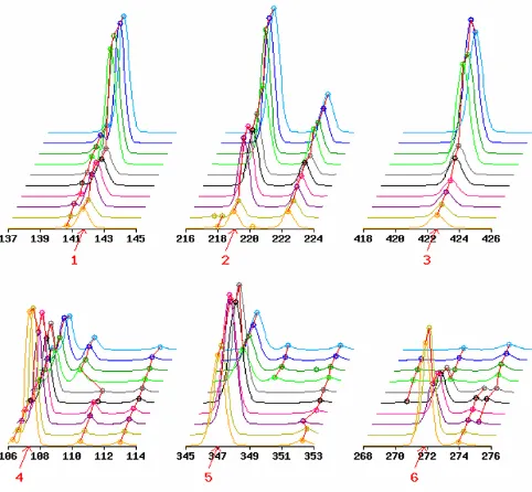
We used a special statistic called GOGOTstat (equation 4) for the detection of differentially expressed TDFs (see Methods). The statistic gives a nonnegative score, with the value 0 for TDFs expressed uniformly in all the interro-gated samples and a high score for differential expression. Of course, there are many ways to rank TDFs according to the degrees of their differential expression. For example, a
t-like statistic (equation 5) obtained by substituting the standard deviation of peak heights in replicate experi-ments for the ratio in equation 4 can be considered. How-ever, such a t-like statistic often gives a high score (rank) to questionable TDFs whose overall peak heights are quite low (Additional file 1). This high score is mainly caused by a low value for the denominator in the t-like statistic. We do not give high scores to these questionable TDFs for the following two reasons. One is they have high relative error (low signal-to-noise ratio). In general, relative error increases for low peak heights when the peak height approaches the background level [31]. The reliability of such candidates is thus implausible [32]. The other reason is the disagreement with visual evaluation (Additional file 2 and Fig. 5). Unlike in microarray analysis, the true sig-nificance of the candidate patterns obtained from high-dimensional electrophoretic data such as HiCEP or Differ-ential Display must be confirmed visually. It is important to develop a score metric compatible with visual evalua-tion. Our statistic (GOGOTstat) is a straightforward appli-cation of this idea.
Table 1 lists expression data (peak heights) and the statis-tics for the top ten TDFs. As expected, there is a wide range of peak heights across time points and high reproducibil-ity between the replicates for each time point. Visual eval-uation of those local electrophoretic patterns also demonstrates that peak alignment is correctly performed (see Fig. 5). The expression data (peak heights) and two statistics (GOGOTstat and t-like statistic) for all 10,624 TDFs in the HiCEP expression matrix are available in Additional file 1.
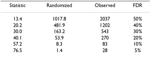
Since the detection of differentially expressed TDFs is based on the HiCEP expression matrix, we can estimate the false discovery rate (FDR), defined as the expected pro-portion of false positives among true differentially expressed TDFs [33]. The random permutation test sug-gests that tens of top-ranked TDFs have statistical signifi-cance at low (5–10%) FDR (see Table 2). Visual evaluation confirmed the validity of the differential expression patterns for the top 100 TDFs and the non-dif-ferential patterns for the last 100 TDFs (data not shown except for the top six TDFs).
Note that there must be other differentially expressed TDFs (i.e., true-negative TDFs) which are not included in the dataset (i.e., the 10,624 TDFs in the expression matrix)
because they do not satisfy the above three conditions used in Step 3. For example, we cannot identify differen-tially expressed TDFs if peaks constituting an identical TDF are not detected due to the effect of a preset detection limit, with the current settings used for the selection of the 10,624 TDFs. Of course, they should be detected if they are genuine. However, as also discussed in the selection of the 10,624 TDFs, the more true-negatives you want to detect, the more tedious visual inspections you have to do. It's a tradeoff.
In practice one may want to detect the differentially expressed TDFs having no data at time point k due to rea-sons such as the above, though the current analysis does not analyze those TDFs. One way to deal with them would be to let Hk = constant (e.g., the predetermined value of the
peak detection threshold). Of course, there are many pos-sible ways to analyze those TDFs. Further improvement of GOGOTstat to make it universal remains to be done.
Conclusion
We propose an integrated strategy (called GOGOT) for identifying differentially expressed TDFs from HiCEP time-course data. As with mass spectrometry data, there remains the problem that the same peaks across electro-pherograms are not perfectly aligned in general [34,35]. We demonstrated that the application of GOGOTnormL Expression patterns of top six TDFs listed in Table 2
Figure 5
(step 1) dramatically contributes to successful peak align-ment via clustering (step 2) and facilitates visual evalua-tion (Figs. 1 and 2). This enabled us to construct a HiCEP expression matrix consisting of 10,624 valid TDFs and ten samples from a total of 256 sets of ten HiCEP electro-phoretic data samples. Normalization of peak heights in the matrix using GOGOTnormH increased reproducibil-ity between replicate experiments (Figs. 3 and 4). These results facilitate the use of various analysis methods for the identification of differentially expressed genes in microarray data.
We used a simple statistic (GOGOTstat at step 4) to rank TDFs according to the degree of their temporal expression change. Researchers involved in HiCEP analysis were very satisfied with the ranking of the differentially expressed TDFs (Fig. 5). Although the current statistic was developed for analyzing HiCEP data, it can also be applied to micro-array data since the input data (expression matrix) is the same. As future work, it would be interesting to evaluate
the potential of the statistic in the analysis of microarray data.
The current method GOGOT can be regarded as a method for analyzing 1-D electrophoretic data. There are a number of methods for analyzing 1-D electrophoretic data produced by various experimental technologies [19,21-29]. Compared to them, GOGOT can be posi-tioned a method specialized for cDNA-AFLP data analysis. The fully automated GOGOT procedure dramatically increased the throughput of data analysis (approximately, 20–30 times). We also verified the power of the strategy using other HiCEP datasets (data not shown). In addition to cDNA-AFLP data, the algorithm should be easily appli-cable to other one-dimensional electrophoretic data such as Differential Display or AFLP. GOGOT can be a power-ful tool for detecting differentially expressed TDFs from multiple one-dimensional electrophograms.
Methods
Data
Samples were prepared from mouse embryonic stem (ES) cells at 0, 12, 24, 48, and 96 h after removal of leukemia inhibitory factor (LIF) from the culture medium. The sam-ples subjected to HiCEP reaction were technically dupli-cated (i.e., the replicates were from the same samples). We thus designated each sample as 0h-1, 0h-2, 12h-1, 12h-2,
24h-1, 24h-2, 48h-1, 48h-2, 96h-1, and 96h-2. The HiCEP reaction was performed according to a previous report [8]. Most of the steps are the same as in standard AFLP [2] except for (i) the primers, whose GC content is 55% to 60% and (ii) the annealing temperature (71.5°C) in selec-tive PCR [8].
cDNA prepared from mRNA extracted from each sample were digested with two 4-bp-cutting endonucleases (MspI combined with MseI) and ligated with the corresponding adaptors. The resulting HiCEP templates, 5'-MspI-MseI-3'
Table 2: Numbers of TDFs called significant at various thresholds.
Statistic Randomized Observed FDR
13.4 1017.8 2037 50%
20.2 481.9 1202 40%
30.0 163.2 543 30%
40.1 53.9 270 20%
57.2 8.3 83 10%
76.5 1.4 28 5%
Statistic: score of GOGOTstat satisfying given FDRs.
Randomized: average number called significant by analyzing 1,000 randomly permutated HiCEP expression matrices.
Observed: number called significant by analysing the original HiCEP expression matrix of 10,624 TDFs and 10 samples.
The FDR is defined as the percentage of falsely significant TDFs compared to the TDFs called significant.
Table 1: Expression data for top ten TDFs ranked by GOGOTstat. Statistic: score of GOGOTstat. The values of peak heights after GOGOTnormH normalization are shown.
Rank Peak height Statistic
H0h-1 H0h-2 H12h-1 H12h-2 H24h-1 H24h-2 H48h-1 H48h-2 H96h-1 H96h-2
1 134 121 228 236 183 186 811 828 843 817 134.7
2 115 115 483 489 388 425 554 870 881 873 134.0
3 91 88 105 112 189 201 704 698 868 706 129.0
4 938 894 650 710 455 485 214 237 295 233 123.7
5 636 627 865 835 712 756 231 247 248 261 116.8
6 719 752 285 282 203 172 16 12 16 10 116.6
7 803 811 320 332 293 299 188 203 212 180 114.9
8 141 153 335 353 342 338 743 763 646 774 112.7
9 643 627 600 634 560 527 90 84 65 72 106.5
fragments, were amplified using fluorescently labeled primers. In total, 256 primer combinations (16 MspI-NN primers combined with 16 NN-MseI primers; N = {A, T, G, C}) were used in the HiCEP analysis. The details of the protocol of the HiCEP reaction are described elsewhere [8].
The PCR products were denatured and loaded on an ABI Prism 310 (Applied Biosystems) for capillary gel electro-phoresis. The digitized images were noise-reduced and baseline-corrected by the GeneScan software (Applied Biotech). After noise reduction and baseline correction, the software quantifies each TDF F by fragment length L
(in bp), peak height H, and area A (in arbitrary units) in the size calibration range (35–700 bp in this analysis). Accordingly, the data obtained from a HiCEP electrophe-rogram consists of a collection of TDFs and each TDF (or
peak) (i = 1,..., nk) in electropherogram Pk (k = 1,..., m;
m = 10 in this case) is characterized by (Li, Hi, Ai)k, where
the peaks are originally numbered with respect to their sizes.
To correct fragment sizing errors caused by the mis-selec-tion of size marker peaks, the preprocessing method of Kadota et al. [12] was adopted. Accordingly, the variation in the lengths of subjectively identical TDFs in the input data was small (± 1 bp at most; see Fig. 1).
Normalization of peak fragment lengths (Step 1; GOGOTnormL)
The purpose of step 1 using GOGOTnormL is to correct peak fragment lengths L across electropherograms so that the corrected lengths L' for subjectively identical TDFs are close to each other. The output data for the m electrophe-rograms (k = 1,..., m) to be compared is represented as (L',
H, A)k. The normalization is performed for each
electro-pherogram Pk (k = {1,..., m}) using a moving window
approach. Briefly, the procedure is as follows:
Step 1-1. Determination of the window (range) in the target electropherogram
Each electropherogram can be approximated by a Gaus-sian kernel using the input data (L, H, A). The approxi-mate electropherogram P(t), which is composed of n
fragments Fi (i = 1,..., n), at length t (in bp) is given by
, where σi =
Ai/(Hi ), the standard deviation of the Gaussian curve approximated to the shape of the Fi.
A total of (ntarget - T + 1) ranges are defined from a target electropherogram Ptarget (target = {1,..., m}), where n
target is
the number of fragments in Ptarget. The ith (i = 1,..., n
target - T
+ 1) range consists of T fragments Fa (a = i,..., i+T-1). In this analysis, we let T = 8 though other numbers are of course possible. For example, the first range consists of eight fragments F1, F2,..., F8 and the (ntarget - T + 1)th range
consists of . The ith range in
the target electropherogram, (starti-endi bp)target, is given
by:
Step 1–2. Selection of the reference for each range
The selection of the reference electropherogram (a kind of typical electrophoretic pattern) for the normalization of the ith range (start
i-endi bp)target is performed according to
Kadota et al. [12]. Briefly, quality scores Q( ) at frag-ment lengths in electropherogram Pk (k = {1,..., m})
are estimated by a windowing calculation of local average correlation coefficients between Pk and the other
electro-pherograms (for details, see [12]). A high (or low) score for electropherogram Pk indicates a high (or low) level of
relative similarity between the electropherogram and the
others at around length . The reference to the ith range
(starti-endi bp)target is the electropherogram Pk (k = {1,...,
m}) satisfying both (i) the number of peaks satisfying
starti ≤ ≤ endi is T/2 or more and (ii) the average quality
score is the maximum.
Step 1–3. Normalization of the target electropherogram
For the ith (i = 1,..., n
target - T + 1) range (starti-endi bp),
GOGOTnormL searches for the sub-electropherogram
Ptarget [start
i+xi, endi+xi] (in the target electropherogram)
that is most similar to the reference Preference [start i, endi]
around the range. The most similar sub-electropherogram is the one that achieves the highest correlation coefficient
ri between Preference [start
i, endi] and the various candidates
Ptarget [start
i+x, endi+x] (-D <= x <= +D). xi is the x at the
highest correlation coefficient ri. We set D = 2, as a maxi-mal realistic displacement.
Fik
P t A t L
i n i i
i i
( ) max
( ) exp
( )
, ,..., /
= − −
=1 2 1 2
2
2
2 2
σ π σ
2π
Fn Fn Fn
target−7, ,..., target−6 target
start L L L L L i
L
i i i i i i i
i i
= − − − < >
−
− −
( )/ ,
,
1 2 2 1 1
2
if and
else σ σ
eendi L L L L L i n
i T i T i T i T i T i T
= + −1+( + − + −1)/2 if + −1+2σ+ −1> + and < ttarget else
− +
+ − + −
T Li T i T
, ,
1 2σ 1
(1)
Lki
Lki
Lki
Lka
If we use a moving window of T fragments, most frag-ments (ntarget-2T+2 fragments) (i = T, T+1,..., ntarget
- T+1) have T values of xa and ra (a = i-T+1, i-T+2,..., i).
Li' (Li in the target electropherogram after normalization) is obtained from Li' = Li - ci. The correction term ci is
calcu-lated by using xa and ra (a = i-T+1, i-T+2,..., i):
where w(ra) is the tricube weight function of ra, namely
w(ra) = 1 - (1 - )3.
Peak alignment via clustering (Step 2)
The major difficulty in one-dimensional (1-D) electro-phoretic data (including HiCEP) analysis is the alignment of multiple peak sets. In order to solve this problem, we here use complete-linkage hierarchical clustering, since the strategy was successfully applied to mass spectrometry data by Tibshirani et al. [20]. To our knowledge, it is the first time clustering-based peak alignment has been used for 1-D electrophoretic data analysis.
The absolute difference in fragment lengths between two peaks is used as the distance. To guarantee that each clus-ter represents individual TDFs, two clusclus-ters are merged only when all the peaks in the two clusters are derived from different samples. Since we analyze ten samples, the maximum peak number in each cluster is thus ten. The dendrogram is cut off at height u bp. In this study, we set
u = 2, implying that every peak in the cluster is at most 2 bp from any other peak in that same cluster by virtue of the use of complete-linkage.
As previously mentioned by Tibshirani et al. [20], the idea for peak alignment is that tight clusters should represent identical TDFs. The use of clustering-based peak align-ment combined with the correction of peak fragalign-ment lengths by GOGOTnormL was successful (Figs. 1 and 2).
Normalization of peak heights (Step 3; GOGOTnormH)
As shown in Fig. 3a, the conventional normalization strat-egy [12,28], in which average peak heights of all the reported TDFs among samples are adjusted, sometimes does not work well. We assert the reason is the use of all the reported TDFs in individual samples. GOGOTnormH selects TDFs satisfying the following three conditions:
(i) peaks corresponding to identical TDFs are exhibited by all samples. The idea is essentially the same as that of Fushiki et al. [35]: peaks exhibited by only a few samples
may just be noise, but peaks exhibited by many subjects appear to be true TDFs.
(ii) the neighboring TDFs are not so close. Suppose that (a) individual TDFs in a set of electropherograms are numbered with respect to their average sizes, (b) there are
m (10 in this case) peaks in the ith TDF (i = 1,..., n
TDF) by
condition (i), and (c) the ten peaks corresponding to the
ith TDF (i = 1,..., n
TDF) in electropherograms Pk (k = 1,..., m)
are characterized by length , peak height ,
area , and standard deviation
. The width of the ith TDF is
defined as
Finally, the TDFs satisfying following conditions are selected:
• Case i = 1,
• Case i = 2,..., nTDF -1,
and
• Case i = nTDF,
(iii) all of the quality scores Q( ) assigned for the ten peaks corresponding to the ith TDF are 0.7 or more. The
score provides an objective goodness for the estimation of
the fragment lengths and our previous study
sug-gests the value of 0.7 is the minimum necessary for the Fitarget
c x w r
w r
i
a a i T i
a
a a i T i = = − + × = − +
∑
∑
1 1 ( ) ( ) , (2)ra3
LkTDF
i HTDF
k
i
ATDFk i
σTDFk π
TDF k
TDF k
i(=A i (H i 2 ))
[min{LTDF . TDF,...,LmTDF . TDFm },max{LTDF .
i i i i i
1 −1 5σ1 −1 5σ 1 +155σ1 1 5σ TDF TDF
m
TDF m
i,...,L i+ . i}].
max{ . ,..., . }
min{
L L
L
TDF TDF TDF m
TDF m
TDF
i i i i
i
1 1
1
1 5 1 5
1 1
+ + <
−
+
σ σ
..5 ,..., 1 5. }
1 1 1
1
σTDF mTDF σ
TDF m
i+ L i+ − i+
max{ . ,..., . }
min{
L L
L
TDF TDF TDF m
TDF m
TDF
i i i i
i
1 1
1
1 5 1 5
1 1
+ + <
−
+
σ σ
..5 ,..., 1 5. }
1 1 1
1
σTDF mTDF σ
TDF m
i+ L i+ − i+
min{ . ,..., . }
max{
L L
L
TDF TDF TDF m
TDF m
TDF
i i i i
i
1 1
1
1 5 1 5
1 1
− − >
+
−
σ σ
..5 ,..., 1 5. }
1 1 1
1
σTDF mTDF σ
TDF m
i− L i− + i−
min{ . ,..., . }
max{
L L
L
TDF TDF TDF m
TDF m
TDF
i i i i
i
1 1
1
1 5 1 5
1 1
− − >
+
−
σ σ
..5 ,..., 1 5. }
1 1 1
1
σTDF mTDF σ
TDF m
i− L i− + i−
LkTDF i
accurate alignment of valid TDFs across electrophero-grams [12].
The peak height after normalization (H') is obtained from
H' = H × N, where N is a normalization factor. The nor-malization factor Nk for electropherogram Pk is calculated
by
where is the average peak height for the selected
TDFs in electropherogram Pk. After normalization, the
average peak height in each electropherogram is adjusted to 100.
Identification of differentially expressed TDFs (Step 4; GOGOTstat)
The differentially expressed TDFs are detected from a total of 10,624 valid TDFs used for peak height normalization at step 3. Consider one expression vector H consisting of peak heights Hp-q at the qth replicate experiment (q = 1,
2,..., np) in time point p. To quantify the degree of
differ-ential expression, we define a statistic GOGOTstat as
where is the average of np normalized peak heights at time point p and Hp-q is the normalized peak height in the
qth replicate experiment at time point p. Since each TDF
has ten normalized peak heights in five time points (i.e.,
p = (0h, 12h, 24h, 48h, 96h)) and each time point has two replicates (i.e., np = 2), the generalized expression vector can be written as H = (H0h-1, H0h-2,..., H96h-2). For example,
the statistic of the top-ranked TDF shown in Table 1 is cal-culated as follows:
The t-like statistic compared to our GOGOTstat statistic (see Results and discussion) is defined as
where σp is the standard deviation of n
p normalized peak
heights at time point p.
Competing interests
The author(s) declare that they have no competing inter-ests.
Authors' contributions
KK invented the method and wrote the paper. RA, YN, and MA provided critical comments and led the project.
Additional material
Acknowledgements
We would like to thank A. Nifuji for visual evaluation of the GOGOT results and J.J. Rodrigue for editing the English. This study was performed through Special Coordination Funds for Promoting Science and Technology of the Ministry of Education, Culture, Sports, Science and Technology, the Japanese Government. This study was also supported by a Research Revo-lution 2002 on Innovative Development Project grant and a Grant-in Aid for Young Scientists (B) (19700273) to K. Kadota from the Ministry of Edu-cation, Culture, Sports, Science and Technology, the Japanese Government.
References
1. Liang P, Pardee AB: Differential display of eukaryotic messen-ger RNA by means of the polymerase chain reaction. Science 1992, 257:967-971.
2. Vos P, Hogers R, Bleeker M, Reijans M, van de Lee T, Hornes M, Fri-jters A, Pot J, Peleman J, Kuiper M, Zabeau M: AFLP: a new tech-nique for DNA fingerprinting. Nucleic Acids Res 1995,
23:4407-4414.
3. Bachem CW, van der Hoeven RS, de Bruijn SM, Vreuqdenhil D, Zabeau M, Visser RG: Visualization of differential gene expres-sion using a novel method of RNA fingerprinting based on AFLP: analysis of gene expression during potato tuber devel-opment. Plant J 1996, 9:745-753.
4. Donson J, Fang Y, Espiritu-Santo G, Xing W, Salazar A, Miyamoto S, Armendarez V, Volkmuth W: Comprehensive gene expression analysis by transcript profiling. Plant Mol Biol 2002, 48:75-97. 5. Breyne P, Dreesen R, Cannoot B, Rombaut D, Vandepoele K,
Rom-bauts S, Vanderhaeghen R, Inze D, Zabeau M: Quantitative cDNA-AFLP analysis for genome-wide expression studies. Mol Genet Genomics 2003, 269:173-179.
6. Yao YX, Li M, Liu Z, Hao YJ, Zhai H: A novel gene, screened by cDNA-AFLP approach, contributes to lowering the acidity of fruit in apple. Plant Physiol Biochem 2007 in press.
N
H
k
selected k
=100 ,
(3)
Hselectedk
GOGOTstat H H
H H
p p
p q p q p q
= −− −
∑
max( ) min( )
max( ) min( ) ,
,
(4)
Hp
GOGOTstat=max(127 5 232 184 5 819 5 830. , , . , . , ) min(− 127 5 23. , 22 184 5 819 5 830
134 121 236 228 186 183 828 8
, . , . , ) ( / ) (+ / ) (+ / ) (+ /111 843 817 830 127 5
5 21 134 7
) ( / ) .
. .
+ = − =
t H H
p p
p p h h h h h
− = −
=
∑
like statistic max( ) min( ) ,
, , , , σ
0 12 24 48 96
(5)
Additional File 1
Expression data for 10,624 valid TDFs. Peak heights after
GOGOT-normH for 10,624 valid TDFs are provided. It also contains two statistics measured by GOGOTstat and a t-like statistic and their ranks. Click here for file
[http://www.biomedcentral.com/content/supplementary/1748-7188-2-5-S1.xls]
Additional File 2
Expression patterns of top six TDFs ranked by a t-like statistic. Legends
are the same as given in Fig. 5. Click here for file
Publish with BioMed Central and every scientist can read your work free of charge
"BioMed Central will be the most significant development for disseminating the results of biomedical researc h in our lifetime."
Sir Paul Nurse, Cancer Research UK
Your research papers will be:
available free of charge to the entire biomedical community
peer reviewed and published immediately upon acceptance
cited in PubMed and archived on PubMed Central
yours — you keep the copyright
Submit your manuscript here:
http://www.biomedcentral.com/info/publishing_adv.asp
BioMedcentral
7. Cnudde F, Hedatale V, de Jong H, Pierson ES, Rainey DY, Zabeau M, Weterings K, Gerats T, Peters JL: Changes in gene expression during male meiosis in Petunia hybrida. Chromosome Res 2006,
14:919-932.
8. Fukumura R, Takahashi H, Saito T, Tsutsumi Y, Fujimori A, Sato S, Tatsumi K, Araki R, Abe M: A sensitive transcriptome analysis method that can detect unknown transcripts. Nucleic Acids Res 2003, 31:e94.
9. Mitani Y, Suzuki K, Kondo K, Okumura K, Tamura T: Gene expres-sion analysis using a modified HiCEP method applicable to prokaryotes: A study of the response of Rhodococcus to iso-niazid and ethambutol. J Biotechnol 2006, 123:259-272. 10. Takahashi H, Umeda N, Tsutsumi Y, Fukumura R, Ohkaze H, Sujino
M, van der Horst G, Yasui A, Inoue ST, Fujimori A, Ohhata T, Araki R, Abe M: Mouse dexamethasone-induced RAS protein 1 gene is expressed in a circadian rhythmic manner in the suprach-iasmatic nucleus. Brain Res Mol Brain Res 2003, 110:1-6. 11. Araki R, Takahashi H, Fukumura R, Sun F, Umeda N, Sujino M, Inoue
SI, Saito T, Abe M: Restricted expression and photic induction of a novel mouse regulatory factor X 4 transcript in the suprachiasmatic nucleus. J Biol Chem 2004, 279:10237-10242. 12. Kadota K, Fukumura R, Rodrigue JJ, Araki R, Abe M: A
normaliza-tion strategy applied to HiCEP (an AFLP-based expression profiling) analysis: Toward the strict alignment of valid frag-ments across electrophoretic patterns. BMC Bioinformatics 2005, 6:43.
13. Wakayama S, Jakt ML, Suzuki M, Araki R, Hikichi T, Kishigami S, Ohta H, Van Thuan N, Mizutani E, Sakaide Y, Senda S, Tanaka S, Okada M, Miyake M, Abe M, Nishikawa SI, Shiota K, Wakayama T: Equivalency of nuclear transfer-derived embryonic stem cells to those derived from fertilized mouse blastcyst. Stem Cells 2006,
24:2023-2033.
14. Araki R, Nakahara M, Fukumura R, Takahashi H, Mori K, Umeda N, Sujino M, Inouye SI, Abe M: Identification of genes that express in response to light exposure and express rhythmically in a circadian manner in the mouse suprachiasmatic nucleus.
Brain Res 2006, 1098:9-18.
15. Araki R, Fukumura R, Sasaki N, Kasama Y, Suzuki N, Takahashi H, Tabata Y, Saito T, Abe M: More than 40,000 transcripts includ-ing novel and non-codinclud-ing transcripts in mouse embryonic stem cells. Stem Cells 2006, 24:2522-2528.
16. Augustynowicz E, Gzyl A, Szenborn L, Banys D, Gniadek G, Slusarczyk J: Comparison of usefulness of randomly amplified polymor-phic DNA and amplified-fragment length polymorphism techniques in epidemiological studies on nasopharyngeal carriage of non-typable Haemophilus influenzae. J Med Micro-biol 2003, 52:1005-1014.
17. Ernst J, Bar-Joseph Z: STEM: a tool for the analysis of short time series gene expression data. BMC Bioinformatics 2006, 7:191. 18. Kadota K, Ye J, Nakai Y, Terada T, Shimizu K: ROKU: a novel
method for identification of tissue-specific genes. BMC Bioin-formatics 2006, 7:294.
19. Higasa K, Kukita Y, Baba S, Hayashi K: Software for machine-inde-pendent quantitative interpretation of SSCP in capillary array electrophoresis (QUISCA). Biotechniques 2002,
33:1342-1348.
20. Tibshirani R, Hastie T, Narasimhan B, Soltys S, Shi G, Koong A, Le QT: Sample classification from protein mass spectrometry, by 'peak probability contrasts'. Bioinformatics 2004,
20:3034-3044.
21. Aittokallio T, Ojala P, Nevalainen TJ, Nevalainen O: Analysis of sim-ilarity of electrophoretic patterns in mRNA differential dis-play. Electrophoresis 2000, 21:2947-2956.
22. Aittokallio T, Ojala P, Nevalainen TJ, Nevalainen O: Automated detection of differently expressed fragments in mRNA dif-ferential display. Electrophoresis 2001, 22:1935-1945.
23. Aittokallio T, Pahikkala T, Ojala P, Nevalainen TJ, Nevalainen O: Elec-trophoretic signal comparison applied to mRNA differential display analysis. Biotechniques 2003, 34:116-122.
24. Aittokallio T, Ojala P, Nevalainen TJ, Nevalainen OS: Automated pattern ranking in differential display data analysis. Methods Mol Biol 2006, 317:111-122.
25. Glasbey C, Vali L, Gustafsson J: A statistical model for unwarping of 1-D electrophoresis gels. Electrophoresis 2005, 26:4237-4242.
26. Drury HA, Green P, McCauley BK, Olson MV, Politte DG, Thomas LJ Jr: Spatial normalization of one-dimensional electrophoretic gel images. Genomics 1990, 8:119-126.
27. Bajla I, Hollander I, Fluch S, Burg K, Kollar M: An alternative method for electrophoretic gel image analysis in the Gel-Master software. Comput Methods Programs Biomed 2005,
77:209-231.
28. Hong Y, Chuah A: A format for databasing and comparison of AFLP fingerprint profiles. BMC Bioinformatics 2003, 4:7. 29. Venkatesh B, Hettwer U, Koopmann B, Karlovsky P: Conversion of
cDNA differential display results (DDRT-PCR) into quantita-tive transcription profiles. BMC Genomics 2005, 6:51.
30. Metsis A, Andersson U, Bauren G, Ernfors P, Lonnerberg P, Montelius A, Oldin M, Pihlak A, Linnarsson S: Whole-genome expression profiling through fragment display and combinatorial gene identification. Nucleic Acids Res 2004, 32:e127.
31. Quackenbush J: Microarray data normalization and transfor-mation. Nat Genet 2002, 32(Suppl):496-501.
32. Breitling R, Armengaud P, Amtmann A, Herzyk P: Rank products: a simple, yet powerful, new method to detect differentially regulated genes in replicated microarray experiments. FEBS Lett 2004, 573:83-92.
33. Benjamini Y, Hochberg Y: Controlling the false discovery rate: a practical and powerful approach to multiple testing. J Royal Statist Soc 1995, 57:289-300.
34. Yasui Y, McLerran D, Adam BL, Winget M, Thornquist M, Feng Z: An automated peak identification/calibration procedure for high-dimensional protein measures from mass spectrome-ters. J Biomed Biotechnol 2003, 4:242-248.
35. Fushiki T, Fujisawa H, Eguchi S: Identification of biomarkers from mass spectrometry data using a "common" peak approach.