Open Access
Research
Local sequence alignments statistics: deviations from Gumbel
statistics in the rare-event tail
Stefan Wolfsheimer*
1,2, Bernd Burghardt
1and Alexander K Hartmann
1,2Address: 1Institut für Theoretische Physik, Universität Göttingen, 37077, Göttingen, Friedrich-Hund-Platz 1, Germany and 2Institut für Physik,
Universität Oldenburg, 26111, Oldenburg, Germany
Email: Stefan Wolfsheimer* - [email protected]; Bernd Burghardt - [email protected]; Alexander K Hartmann - [email protected]
* Corresponding author
Abstract
Background: The optimal score for ungapped local alignments of infinitely long random sequences is known to follow a Gumbel extreme value distribution. Less is known about the important case, where gaps are allowed. For this case, the distribution is only known empirically in the high-probability region, which is biologically less relevant.
Results: We provide a method to obtain numerically the biologically relevant rare-event tail of the distribution. The method, which has been outlined in an earlier work, is based on generating the sequences with a parametrized probability distribution, which is biased with respect to the original biological one, in the framework of Metropolis Coupled Markov Chain Monte Carlo. Here, we first present the approach in detail and evaluate the convergence of the algorithm by considering a simple test case. In the earlier work, the method was just applied to one single example case. Therefore, we consider here a large set of parameters:
We study the distributions for protein alignment with different substitution matrices (BLOSUM62 and PAM250) and affine gap costs with different parameter values. In the logarithmic phase (large gap costs) it was previously assumed that the Gumbel form still holds, hence the Gumbel distribution is usually used when evaluating p-values in databases. Here we show that for all cases, provided that the sequences are not too long (L > 400), a "modified" Gumbel distribution, i.e. a Gumbel distribution with an additional Gaussian factor is suitable to describe the data. We also provide a "scaling analysis" of the parameters used in the modified Gumbel distribution. Furthermore, via a comparison with BLAST parameters, we show that significance estimations change considerably when using the true distributions as presented here. Finally, we study also the distribution of the sum statistics of the k best alignments.
Conclusion: Our results show that the statistics of gapped and ungapped local alignments deviates significantly from Gumbel in the rare-event tail. We provide a Gaussian correction to the distribution and an analysis of its scaling behavior for several different scoring parameter sets, which are commonly used to search protein data bases. The case of sum statistics of k best alignments is included.
Published: 11 July 2007
Algorithms for Molecular Biology 2007, 2:9 doi:10.1186/1748-7188-2-9
Received: 5 October 2006 Accepted: 11 July 2007 This article is available from: http://www.almob.org/content/2/1/9
© 2007 Wolfsheimer et al; licensee BioMed Central Ltd.
Background
Sequence alignment is a powerful tool in bioinformatics [1,2] to detect evolutionarily related proteins by compar-ing their sequences of amino acids. Basically one wants to determine the "similarity" of the sequences. For example, given a protein in a database like PDB [3], such similarity analysis can be used to detect other proteins, which are evolutionary close to it. Related approaches are also used for the comparison of DNA sequences, i.e. shotgun DNA sequencing [4], but the application to DNA is not consid-ered in this article.
Alignment algorithms find optimum alignments and maximum alignment scores S of two or more sequences for a given scoring system. Needleman and Wunsch sug-gested a method to compute global alignments [5], whereas the Smith-Waterman algorithm [6] aims at find-ing local similarities. Insertions and deletions of residues are taken into account by allowing for gaps in the align-ment. Gaps yield a negative contribution to the alignment score and are usually modeled by a gap-length l depend-ing score function g (l). Widely used are affine gap costs because for two given sequences of length L and M, because fast algorithms with running time (LM) are available for this case [7]. Note that for database queries even this is too complex, hence fast heuristics like BLAST [8] are used there.
By itself, the alignment score, which measures the similar-ity of two given sequences, does not contain any informa-tion about the statistical significance of an alignment. One approach to quantify the statistical significance is to compute the p-value for a given score S. This means under a random sequence model one wants to know the proba-bility for the occurrence of at least one hit with a score S greater than or equal to some given threshold value b, i.e. (S ≥b). Often E-values are used instead. They describe the number of expected hits with a score greater than or equal to some threshold value. One possible access to the statis-tical significance can be achieved under the null model of random sequences. Then the optimal alignment score S becomes a random variable and the probability of occur-rence of S under this model P (s) = (S = s) provides esti-mates for p-values. Analytic expressions for P (s) are only known asymptotically in the case of gapless alignments of long sequences, where an extreme value distribution (also called Gumbel distribution) [9,10] was found. For align-ments with gaps, such analytical expressions are not avail-able. Approximation for scenarios with gaps based on probabilistic alignment [11-13], large deviations [14] and a Poisson model [15] had been developed. Altschul and Gish [16] investigated the score statistics of random sequences for a number of scoring systems and gap
parameters by computer simulations: They obtained his-tograms of optimum scores for randomly sampled pairs of sequences by simple sampling. By curve fitting, they showed that in the region of high probability the extreme value distribution describes the data well, also for gapped alignments of finite sequences. Additionally, they found that the theoretical predictions for the relation between the scoring system on one side and the Gumbel parame-ters on the other side hold approximately for gapped alignments. In this context they obtained two improve-ments: Using a correction to account for finite sequence lengths and sum statistics of the k-best alignments, theo-retical predictions for ungapped alignments could be applied more accurately to gapped alignments. Recently Olsen et al. introduced the "island method" [17,18], which accelerates sampling time. BLAST [8] uses precom-puted data, generated with the island method, to estimate E-values. In any case, as already pointed out, the studies in Ref. [16] and [18] give reliable data in the region where P (s) is large only. This is outside the region of biological interest because pairs of biologically related sequences have a higher similarity than pairs of purely randomly drawn sequences.
To overcome this drawback a rare-event sampling tech-nique was proposed recently [19], which is based on methods from statistical physics. This general approach allows to obtain the distribution over a wide range, in the present case down to P (s) = 10-40. So far this method has
been applied to one relevant case only, namely protein alignment with the BLOSUM 62 score matrix [7] and aff-ine gap costs with α = 12 opening and β = 1 extension costs. It turned out that at least for one scoring matrix and one set of gap-cost parameters, the distribution deviates from the Gumbel form in the biologically relevant rare-event tail, where simple sampling methods fail. Empiri-cally, a Gaussian correction to the original distribution was proposed for this case.
Results as in Ref. [19] are only useful if one obtains the distribution for a large range of parameter values which are commonly used in bioinformatics. It is the purpose of this work to study the distribution of S for other relevant cases. Here we consider the BLOSUM62 and the PAM250 score matrices in connection with various parameters α , β of affine gap costs.
PAM 250 matrices in conjunction with different affine gap costs. We show also our results for the sum statistics of the k largest alignments. In the last section, we summarize and discuss our results.
Statistics of local sequence alignment
In this section, we define sequence alignment, and state some analytical results for the distribution of the opti-mum scores S over pairs of random sequences.
Let x = x1x2 ... xL and y = y1y2 ... yM be two sequences over a
finite alphabet Σ with r = |Σ| letters(e.g. nucleic acids or amino acids). An alignment is a set = {(ik, jk} of K pairs of "non-crossing" indices (k = 1, 2, ..., K - 1, 1 ≤ik <ik+1 ≤L and 1 ≤jk <jk+1 ≤M) identifying pairs of letters
from the two sequences. Letters, which are not paired are called unpaired or gapped. A gap g of length lg is a substring
of lg gapped letters from one sequence. Note, that this rep-resentation [14] of an alignment is equivalent to an intro-duction of a gap symbol, as commonly used. Formally the gap cost function can be defined by considering the length of a gap beginning at the kth pairing in sequence x or sequence y respectively, in detail
The score (x, y, ) of the local alignment of the two sequences is composed of a sum over all aligned pairs and a sum over all gaps of both sequences:
where σ (a, b) a, b ∈ is the given score matrix (or substi-tution matrix) and g (l) the gap-cost function with g (0) = 0. Note that the alignment is local, because the (possibly large) gaps at the beginning and the end of each sequence are not included in the scoring function. Otherwise the alignment would be global. Here, we consider the BLOSUM62 [20] and the PAM250 [21,22] matrices and affine gap costs, i.e. g (l) = α + β (l -1). The similarity of the sequences is the optimum alignment with the maximum score
which can be obtained in (LM) time [7].
In the case of gapless optimum local alignments of two random sequences of L and M independent letters from Σ with frequencies {fa } with a ∈Σ and ∑a fa = 1, referred as null model, the score statistics can be calculated analyti-cally in the asymptotic regime of long sequences [9,10].
In this case one obtains the Gumbel distribution (Karlin-Altschul statistics) [23]
(S ≥b) = 1 - exp [- KLM e-λb] (3)
or
PGumble (s) = (S = s) = λ KLM exp [-λ s - KLM e-λ s]
(4)
The parameters λ and K of Eq. (3) can be derived directly from the score matrix σ (a, b) and frequencies fa [9,10].
As pointed out by Altschul and Gish [16], in finite systems there occur edge effects: An alignment may extend to the end of either sequence and the score will be distorted towards lower values and high scores become less proba-ble. Since this effect vanishes in the limit of infinite sequences, the tail of Eq. (3) can be understood as an upper bound for finite sequences.
Arratia and Waterman [24] predicted a phase transition between a linear phase and a logarithmic phase, i.e. a lin-ear growth of the excepted score as a function of the sequence length, changing to a logarithmic growth with increasing gap costs. In the linear phase an optimum alignment may spread over a large range of the sequences and the statistical theory breaks down. However, only the logarithmic phase is of interest in biological questions because the alignment algorithm becomes more sensitive in this phase, especially near the threshold [25].
Often the sensitivity of an alignment algorithm can be increased by not only considering the best optimal align-ment score, but also the k-best scores of non overlapping alignments. An (LM) algorithm for this task, based on Sellers concept of local optimality, was developed [26,27]. According to Karlin and Altschul [28] also the sum statis-tics of the k-best alignment scores for random sequences can be derived analytically for asymptotically long sequences. The probability f for the sum of the k-best
nor-
l k i i
l k j j
g x
k k
gy k k
( )
( ) .
= − −
= − −
+
+
1
1
1
1
S
S x y g l
x y g l k
i j g
g k
K
i j gx
k k
k k
( , , ) ( , ) ( )
( , ) { ( (
x y = +
= +
∑
∑
=
σ
σ
gaps 1
)))+ ( ( ))}
= −
=
∑
∑
g l kgyk K
k K
1 1
1
(1)
S( , )x y =max ( , , ),S x y
(2)
malized scores (λ and K are the
corresponding Gumbel-parameters for the optimal align-ment)is given by the integral
In the tail, i.e. for large t, f (t) is well approximated by
In the asymptotic theory the score can be seen as a contin-uous variable and the probabilities Eq. (4) and Eq. (5) become probability densities. Then the probability of finding a normalized score b or larger is given by the
inte-gral . However in computer
simula-tions the score is a discrete variable and therefore the normalization constants in Eq. (5) differ from continious scoring. Below we will compare the results of our numer-ical studies to this distribution in the tail of the data for values k = 2, ..., 5.
Sampling of rare-events
Metropolis Hastings Algorithm
As already pointed out, the main purpose of this paper is to calculate the tail of the distribution of optimum scores of gapped local alignments over pairs of randomly and independently drawn sequences of finite lengths. The basic idea of our approach is to generate the sequences from different distributions, which are biased towards higher scores.
In order to be more precise let us denote the state space of all possible pairs of sequences (x, y) as and an element in this space as a configuration. We write X = (x, y).
The probability mass function (pmf) of finding X under the null model is given by
and the alignment
score as defined in Eq. (2) is a random variable. A direct way to obtain the probability of the occurrence of a cer-tain score s, is to generate n uncorrelated representatives Xi
∈ according to the null model and then compute the expectation values of the family of indicator functions hs:
→⺢ with hs (X) = 1, if S (X) = s and hs (X) = 0 otherwise, in other words
Since the region of biological interest is located in the rare-event tail a huge amount of samples would be needed to achieve an acceptable accuracy. In practice the rare-event tail becomes inaccessible.
Our method is based on importance sampling of a mix-ture of chains based on the Metropolis-Hastings algo-rithm. Before describing the coupling of multiple chains, we introduce the general idea of importance sampling first: The approach is based on sampling from a different distribution, such that the region of interest is sampled with high probability. Since this happens in a controlled manner the true distribution can be obtained afterward, as frequently used in variance reduction techniques. The modified distribution yields a different random variable with a different pmf q. We may write
At least approximately, the distribution of local alignment follows a Gumbel distribution, which exhibits an expo-nential behavior in the tail. Therefore an obvious choice for the biased distribution is
where the unnormalized weight of a configuration, ZT is a (usually unknown) normalization constant and T an adjustable parameter, which we will call "temperature" (In the framework of statistical mechanics, which is closely related to our method, the parameter T describes the temperature of a physical system. The pair of sequences can be seen as a configuration of a physical sys-tem and the negative score as the energy function. Then exp [S (X)/T] refers to the so called Gibbs-Boltzmann distri-bution.) The close-to Gumbel form of the distribution is also directly related to the so called "large deviation rate function", which basically describes the decay rate of the tail of the distribution. Note that, if the score distribution is an exact Gumbel distribution Eq. (3), i.e. the rate func-tion a known constant λ, then setting T = 1/λ in Eq. (7) yields a "flat score histogram" for sufficient large s. Hence, in this case, a simulation at a single carfully chosen value T would be sufficient to obtain the full result. Since P (s) does not follow the Gumbel form exactly, importance sampling has to be applied. Each value of T selects one
Tk=λ
∑
ik Si − KLM λ( ln )
f t e
k k y e dy
t
k y t k
( )
!( )! exp( ) .
( )/
=
− −
−
− −
∞
∫
22
0 (5)
f t e
k k t k t
t
k k
tail( )
!( )![ ( ) )].
=
− − −
−
− −
1 1
1 2 (6)
P(S b) f t dt( ) b
≥ =
∫
∞
p p i fx f
L
y j M
i j
( )X = ( , )x y =
∏
=1∏
=1
P[ ( )S s] E[ ( )]h h( ) ( )p ( ).
n h
s s s i
i n
X X X X X
X
= = =
∑
≈∑
=
1
1
P s S s h p
q q n h
p
s s
i n
i
( ) [ ( ) ] ( ) ( )
( ) ( ) ( )
(
= = = ′ ′
′ ′ ≈ ′
′
′ =
∑
∑
P X X X
X X X
X
X
1
1
ii
i
q ) (X′).
q q X
Z Z p S T
T T
T T
( )X ≡ ( )≡ 1 ( ) exp[ ( )/ ],X ⋅ X (7)
region of the distribution around which a high accurracy is obtained.
This importance sampling approach is conceptual related to the method of "measure change" in large deviation the-ory. For example Siegmund and Yakir [14] approximated the p-value for local sequence alignment by considering the log-likelihood ratio between an alternative measure and the measure of the null model. Under the new meas-ure a rare event occurs more likely than under the original null measure and approximations become possible. Another example can be found in Ref. [29], where tech-niques from large deviation theory were applied to proof "asymptotic efficiency" of rare-event simulations.
However, since there is no direct method to sample directly according to the modified distribution Eq. (7) we implemented the Metropolis-Hastings algorithm [30], which is explained now in detail. It is based on ergodic Markov chain Monte Carlo (MCMC) in state space. Ergodic here means, that for a given state in the configuration space any other can be achieved by stepwise "local" modifica-tions of configuramodifica-tions in finite time. Note that we work in discrete time steps here. Let X ∈ a configuration at time t (e.g. at the start of the simulation). To determine the configuration at time t + 1, first a trial configuration X* is selected randomly among its "neighbors". The neigh-borhood of a configuration depends on the choice of trial steps, which are specified below. For practical reasons we require, that the score within a neighborhood of a given configuration will not change too much. The transition matrix for this trial selection process is denoted by P (X, X*). Now, the trial configuration becomes the configura-tion at time t + 1, i.e. is accepted, with probability
with ∆S = S (X*) - S (X) If the trial configuration is not accepted, the previous configuration X is kept for the next time step t + 1. In this way, the Markov chain fulfills the detailed balance condition P (X*, X) (X* →X)·qT (X*) = P (X, X*) (X → X*)·qT(X). In this case it has been proven that an ergodic Markov chain converges to the sta-tionary distribution qT. Ergodicity means, that there is a non-zero probability for a path between any pair(X1, X2) of configurations.
We used a simple way to define the neighborhood of a configuration and constructed the trial configuration as follows: First a letter a is drawn from the alphabet Σ according to the letter weights fa and next one of the sequences (x or y) and a position i is chosen randomly. Finally, the letter at position i is replaced by a.
Given a Monte Carlo chain (X1, ..., Xn) estimated for a fixed temperature T in principle one may estimate expec-tation values with respect to any member of the family of distributions qT by importance reweighting
Since the normalization of qT is not trivial, we used a dif-ferent normalization
and estimate Z from the sample
. A detailed discussion about
this issue can be found in Ref. [31,32]. In practice this may work badly as soon as the parameter ranges of the given distribution and the target distribution do not overlap suf-ficiently. In this case qT'(Xi) is very small, but the configu-rations where qT' (X)/qT (X) is sufficiently large are not
generated because qT (X) is relatively small for those. Therefore we sampled a mixture of many coupled Monte Carlo chains and reweighted the mixture, which is explained in detail in the next section. This allows for large overlap between neighboring distributions and to determine the normalization constants, up to an irrele-vant global constant.
Metropolis Coupled MCMC
Metropolis Coupled Markov Chain Monte Carlo (MCMCMC) was first invented by Charles Geyer [33] and then rein-vented by Hukushima and Nemoto [34] under the term exchange Monte Carlo. In physical literature MCMCMC is often denoted as parallel tempering. The method has become a standard tool in disordered systems with a rough (free) energy landscape [35]. These rough energy landscapes are characterized by high energy barriers and can be found for problems like protein folding [36-40], nucleation [41], spin-glasses [42,43] and other models characterized by rare events [19,44]. In the last decade it turned out that MCMCMC accelerates equilibration and mixing remarkably.
p P
P q
q
P
T T ( ) max , ( , )
( , ) ( )
( ) max , (
X X X X
X X X
X
→ = ⋅
=
∗ ∗ ∗
∗
1 1 XX X
X X
∗ ∗
, )
( , )exp[ / ] ,
P ∆S T
(8)
p
p
E ′ ′
=
≈
∑
⋅T T i
T i i
n
i
g
n q
q g
[ ( )] ( )
( ) ( )
X X
X X
1
1
E ′ ′
=
≈
∑
⋅T T i
T i i
n
i
g
n q
q g
[ ( )] ( )
( ) ( ),
X X
X X
1
1
(9)
In the framework of MCMCMC m copies X(1), ..., X(m) of
the system held at different temperatures T1 <T2 < ... <Tm are simulated in parallel. This means one samples from the product of the state space m weighted with the joint
distribution with weights . Since the different
copies are allowed to exchange temperatures during the simulation, let us define the space of all possible map-pings from the m configurations to the m temperatures as temperature space.
During the simulation, mainly each of the replicated con-figurations will evolve independently according the underlying MCMC scheme charaterized by the weight Eq. (7) at its current temperature, i.e. according to Eq. (8). In addition to this evolution, every texchangeth step (for each replicated configuration) a flip between two neighboring replicas k and k + 1 is attempted, i.e. for all k ∈ {1, ..., m -1}. If an attempt is successful, the configurations X(k) and
X(k+1) are exchanged (denoted by X(k) ↔ X(k+1)), i.e. the
configurations which has previously evolved at tempera-ture Tk will now evolve at temperature Tk + 1 and vice versa.
This exchange is accepted with the probability
where, , ∆S = S (X(k + 1)) - S (Xk) and all
weights are calculated with the configurations before the flip. This leads to a "random walk in temperature space" of the configurations.
Note that another possible approach based on Markov chains to compute p-values of a random model with a random variable X, [X > b] was introduced by Wilbur [45].
The first step is to sample from an unbiased Markov chain based on the model of interest and compute the median of the (high probability) distribution. In the second itera-tion the random walk is truncated such that only values larger than the median of the first iteration occur. This cor-responds to choosing a lower temperaure T in Eq. (7). The third iteration uses the median of the second iteration and so forth. This is repeated until a fraction of 1/4 of all events lay beyond a certain threshold value leading to a non decreasing sequence of splitting intervals defined by the medians of each iteration. This sequence is used in the second stage of the algorithm, where p-values are com-puted explicitly by multiplying the p-values of the trun-cated distribution in each iteration.
Although this method is easy to implement and errors can be estimated relatively simply, the MCMCMC approach has the advantage that the different configurations are not subjected to a sequence of decreasing temperatures, but perform a random walk in temperature space, i.e. visit all temperatures several times. Thus, mixing is accelerated and hence fewer Monte Carlo steps are required.
Reweighting the mixture
The production run of MCMCMC yield a set of m different chains of lengths nj. We denote the ith configuration in the chain of jth temperature as . Of course this leads to a
larger parameter range than simple importance reweight-ing of a sreweight-ingle chain, hence Eq. (9) cannot be applied directly to the mixture. Geyer [46] developed a generaliza-tion of the importance reweighting formula to mixtures. His idea is based on Eq. (9), where qT is replaced by a "mixture weight" qmix, i.e. (using qj ≡ , i.e. qj represents the unormalized weights)
The (global) normalization constant is given by
. The mixture weight
function is known up to normalization constants :
with n = ∑jnj. The unknown constants c ≡ (c1, ..., cm) may be estimated by reverse logistic regression introduced by Geyer [46]. Here we used an alternative approach to qT j m j =
∏
1 p q q q qk k T k
T k T k T k k k k
X X X
X X ( ) ( ) ( ) ( ) ( )
max , ( )
( ) ( ) ↔
(
+)
= ⋅ + + + 1 1 1 11(( )
max ,exp[ ] ,
( ) X k k S + =
{
−}
11 ∆ ∆β
(10) ∆βk k k T T = − + 1 1 1
X( )ij
qT
j
E ′ ′
= = ≈
∑
∑
⋅ T T i j i j i n j m i j g Z q q g j [ ( )] ( ) ( ) ( ). ( ) ( ) ( ) X X X X 1 1 1 mix (11)Z i qT q
n j m i j i j j
=
∑
=1∑
=1 ′( )/ ( )( ) ( )
X mix X
cj ZT
j ≡ q n n q c j j m j j
mix( )
( ) ,
X = ⋅ X
=
∑
1
Sketch of the graph of overlapping distributions q1,..., q4 Figure 1
Sketch of the graph of overlapping distributions q1,..., q4.
Dis-tant distributions have weak overlaps.
w12 w23 w34
w13 w24
obtain the constants c developed by Meng and Wong [47], which is explained now.
Since the global normalization constant Z in Eq. (11) is trivial, the problem is reduced to the estimation of (m - 1) ratios of normalization constants to some reference value. One possible choice is to fix the normalization constant of q1 and estimate the ratios ri = c1/ci (i = 2, ..., m).
Since the support of the mixture distribution is broader than each of the particular distributions, not all pairs of distributions qi and qj overlap in general. The overlaps of
the empirical data can be measured by the matrix
and the set of distributions can be represented by a graph (V, E) with vertices being the weight functions V = {q1, ..., qm} and the set of all overlaps being the weighted edges E = {wij} with wij > 0(see Fig. 1. We require, that the so con-structed graph is connected. In practice one must find paths between each pair of distributions with not too small weights. In this case each distribution has a finite overlap with qmix and reweighting become possible on the
full support.
Consider arbitrary weight functions αij assigned to each edge of the graph and define the following expectation values with respect to qj
This means, for any given vector c, all values {bji} can be calculated using this expression. We require the αij to be symmetric, i.e. αij = αji, and a finite overlap with each of the distributions. With r1 = 1 and ribji = rjbij it is straight for-ward to construct a linear system for the remaining (m - 1) ratios, for i > 1:
with aii = ∑j ≠i bij and aij = -bij for i ≠j. This equations cannot
be solved directly, because the coefficients aij do depend on the unknown ratios. However it is possible to solve Eq.
(13) self-consistently. Using = (b11, b21,..., bm1) and
including explicitely the dependence on r = (r1, r2,..., rm) we obtain
A (r(t))·r(t + 1) = b(r(t)). (14)
This equation can be solved by starting with r(1) = (1, 1, ...,
1) and iteratively solving for r(t + 1) till convergence.
Fol-lowing the paper of Meng and Wong [47] Eq. (14) with
the choice converges to same
esti-mator as proposed by Geyer [46], which is based on max-imization of a quasi-loglikelihood. The desired probability P (s) can be achieved by setting qT' to the unbi-ased weight q∞= 1 and estimate the expectation values of the indicator functions hS in Eq. (11).
Illustration and convergence diagnostics
In order to guarantee start configurations taken from the stationary distribution the first few iterations of the chains have to be discarded. The number of iterations to be dis-carded is denoted as burning or equilibration period. Usu-ally one starts from a random (i.e. disordered) configuration and equilibrates the system. At the begin-ning of the simulation the system has a low score and hence it can reach in principle most regions of the score landscape. If the temperature is low, one sees when look-ing at Eq. (7) that configurations with large score domi-nate. Hence, typically the score increases or stays the same during the simulation with only few score-decreasing fluc-tuations.
Note that if "ground states" are also known, i.e. the maxima of the score landscape, the reverse process is pos-sible, i.e. starting from a high maximum and sampling its local environment. One can use this fact to verify, whether a system has equilibrated on a larger scale, i.e. whether it is able to overcome the typical barriers in the score land-scape. This is the case when the average behavior for two runs, one starting with a disordered configuration and one starting with an "ground-state" configuration, is the same (within fluctuation). If the temperature is too small, this is usually not possible.
It is helpful to consider a simple toy system to illustrate and benchmark the method, in detail consider a 4-letter alphabet of equal weights and sequence lengths L = M = 10, 20. The scoring system is defined by the score matrix
and affine gap costs with α = 4 and β = 2.
w
n n h h
ij i j
S k i
k n
S
S l j
l n
i j
=
⋅
= =
∑
∑
∑
1
1 1
(X( )) (X( ))
b q
c q q
c c b
ji j i ij
j j i ij
i
j ij
=E [ ( )X ⋅ ( )]X =
∑
( )X ⋅ ( )X ⋅ ( )X = .X
α 1 α
(12)
bi bi ri bji r b r a r
j i
i ij j
j i j
ij j j
1 1
1 1
= ⋅ = ⋅ − ⋅ ≡ ⋅
≠ ≠ > >
∑
∑
∑
,
,
(13)
ˆ b
αij
i j
n n
n q
( )X = ⋅ ( )X
2 mix
σ( , )a b a b.
else
= + =
−
1 3
if
An illustration of the equilibration criterion is given in Fig. 2. By "visual inspection" we obtain equilibration times 100 (T = ∞),1000 (T = 1), 10000 (T = 0.7), 15000 (T = 0.6) and 20000 (T = 0.5), respectively.
A more quantitative method was introduced by Raftery and Lewis [48,49], that estimates equilibration and sam-ple times for a set of quantils. Raftery and Lewis's pro-gram, which is available from StatLib [50] or in the CODA package [51], estimates a thining interval nthin as well. That means only every nthinth step is used for inference in order to avoid correlations between the scores at time t and t +
∆t, that occur in MCMC in constrast to direct generating random sequences. The program requires three parame-ters: the desired accuracy r, the required probability s of attaining the specified accuracy and a less relevant toler-ance parameter ε.
We compared the result of the estimate of the equilibra-tion time with the simple visual approach: For the exam-ple given in Fig. 2 we maximized numerical estimate of equilibration time over a set of quantils between 0.1 and 0.95 for r = 0.0125, s = 0.95, ε = 0.001): The results for the equilibration time obtained by this approach are always much smaller than those obtained by the visual inspec-tion. For example for L = 20, the Rafter-Lewis approach gives an equilibration time of 800 steps for the lowest temperature, whereas Fig. 2 suggests 20000 steps. There-fore equilibrium might not be guaranteed with the Rafter-Lewis approach and the visual inspection seems to be more conservative.
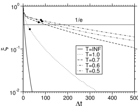
To estimate the times scales over which the simulation decorrelates, we considered the autocorrelation function
denoting the average over different times and
inde-pendent runs. The typical time scale, over which correla-tion vanish is the correlacorrela-tion time τ defined via ξ (τ)= 1/ e. The normalized auto-correlation function for the sys-tem of L = 20 is shown in Fig. 3. A comparison with Raft-ery and Lewis diagnostics of nthin, indicated by dots, gives evidence that the two estimates coincide with each other at least in the order of magnitude. The correlation time increases with decreasing temperature, which corresponds to a growth of the equilibration time with decreasing tem-perature in Fig. 2. However by the generation of the histo-grams the correlations will average out, but estimates of the errors are more complicated when the data are corre-lated. However the consideration of τ and nthin has some practical issues too: For the application it is only necessary to infere every 100 th step, which saves a lot disk space.
Once the equilibration period is estimated one may check the convergence of the remaining parts of the chains to the equilibrium distributions. This was done by computing the Gelman and Rubin shrink factors R [49,52,53]. This diagnostic compares the "within-chain" and the "inter-chain variance" of a set of multiple Monte Carlo "inter-chains.
ξ( )
( ) ( ) ( )
( ) ( )
,
t
S t S t t S t
S t S t
t t
t t
= + −
−
0 0 0
2
0 2 0 2
0 0
0 0
(16)
" t
0
Equilibration of the 4-letter system (L = M = 20) with tem-peratures T = 0.5, 0.6, 0.7, 1.0, ∞ Equilibrium is reached after 20000, 15000, 10000, 1000, 100 steps (indicated by arrows) respectively
Figure 2
Equilibration of the 4-letter system (L = M = 20) with tem-peratures T = 0.5, 0.6, 0.7, 1.0, ∞ Equilibrium is reached after 20000, 15000, 10000, 1000, 100 steps (indicated by arrows) respectively. S (t) is averaged over independent 250 runs.
0 10000 20000 30000 40000
MC-Step
05 10 15 20
S
T=0.6
T=0.7
T=1.0
T=INF T=0.5
Score auto-correlation function for different temperatures (4 letters, L = M = 20)
Figure 3
Score auto-correlation function for different temperatures (4 letters, L = M = 20). Circles indicate corre-sponding nthin
from Raftery and Lewis [48,49].
0 100 200 300 400 500
∆
t
10-2 10-1 100
ξ
T=INFWhen the factor R approaches 1 the within-chain variance dominates and the sampler has forgotten its starting point. For the lowest temperature in our toy model L = 20 we found R = 1.03 for the 99.995% quantile, which appears to be reasonable.
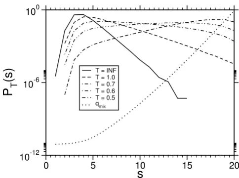
From the equilibrated and converged chains we obtained histograms for different temperatures, which are shown in Fig. 4 for the case L = 20.
The empirical overlap matrix of this mixture is estimated by
which has a finite overlap between all pairs. Note that in general a weaker condition must be fulfilled, namely that a connected path from the lowest to the hightest temper-ature must be possible, as outlined before. In more com-plex models only this condidition might be fulfilled.
Applying the reweighting technique, which was explained in the previous section, we obtain the infinite temperature probability P (s) (see Fig. 5).
Obviously, the toy model has Z = 42 L configurations. The
maximum score over the ensemble of all possible config-urations is Smax = L. This corresponds to a pair of sequences with L equal letters xi = yi (i = 1 ... L). The number of configurations with the highest score is 4L.
Hence, the probability to find a maximum score among all random sequences is P (Smax) = [S = Smax] = 4L/42 L = 4-L.
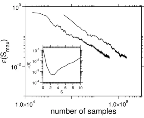
Below, to benchmark the Monte Carlo algorithm, we compare the convergence of the relative error
for different sequence
lengths, Psample (s) being the corresponding probability obtained from the MC simulation. From Fig. 6, which illustrates convergence of the ε (Smax) as a function of total
sample size for all temperatures. In order to get a clear pic-ture we averaged over several blocks of runs.
For small systems one may enumerate all possible config-urations and compare the complete distribution with the Monte Carlo data. The empirical probability distribution for L = 10 in Fig. 5 coincides with the exact result, such that a the difference is not visible in the plot. However L = 10 is a very small system in contrast to real biological sequences, which are considered in section "Results", but exact enumeration is only possible on a modern computer cluster. Hence only for L = 10 the relative error
( )
. . . .
. . . .
. .
wij ≈
1 0 543 0 256 0 098 0 009 0 543 1 0 572 0 266 0 070 0 256 0 572 11 0 624 0 264 0 098 0 266 0 624 1 0 570 0 009 0 070 0 264 0 570 1
. .
. . . .
. . . .
,
(17)
ε( )
( )
max
max
S
P S L
L
= −
−
−
sample 4
4
Score probabilities obtained throw the reweighting mixture technique for a 4-letter system with sequence-length L = 10, 20 and scoring parameters Eq
Figure 5
Score probabilities obtained throw the reweighting mixture technique for a 4-letter system with sequence-length L = 10, 20 and scoring parameters Eq. (15) using affine gap costs (α= 4, β= 2). For L = 10 the P (s) had also been been obtained by exact enumeration of all 42 × 10 configurations. A difference
between the empirical curve is not visible in the plot.
0 5 10 15 20
s
10-12 10-8 10-4 100
P(s)
L=20 L=10
Empirical probabilities for the toy model (4 letters, L = M = 20) held at finite temperature
Figure 4
Empirical probabilities for the toy model (4 letters, L = M = 20) held at finite temperature. The dottet line showes the normalized mixture weight function .
0 5 10 15 20
s
10-1210-6 100
P
T(s)
T = INFT = 1.0T = 0.7 T = 0.6 T = 0.5 qmix
ˆ
(see inset of Fig. 6) can be
computed on the full support. In principle one is able to reduce variance on the low score end of the distribution by introducing negative temperature values, but this is beyond of the scope of this article.
Error estimation
As mentioned previously, a direct calculation of the errors is hardly possible. The first reason is that the Markov chain data are correlated. Secondly, the iterative estima-tion of the relative normalizaestima-tion constants is not trivial and contributes also to the overall error. Nevertheless, one can evaluate errors using the jackknife method [54]: First, in order to ensure, that the data are uncorrelated, we took data points which are seperated by at least the correlation time, determined via Eq. (16). Next, the dataset is divided into nb blocks of equal size (hence, the number should be a multiple of nb). Quantities of interests g are calculated k
times (k = 1 ... nb), each time omitting block Bk. These nb values are averaged over all possibilities of k, in the nota-tion of Eq. (11)
The error of g is estimated by
For example the relative errors of the
normaliza-tion constant ratios increase from 8.6 × 10⁻⁴ for r
2 to 1.29
× 10-2 for r
5. This indicates that the method is able to
cap-ture the error propagation of the relative normalization constants due to weak overlaps of distant distributions (see also Eq. (17)). Similar errors for the probabilities P (s) can be estimated by applying this approach.
Results
Optimal alignment statistics
Next, we show the results from the application of the method to biologically relevant systems: local sequence alignment of protein sequences using BLOSUM62 [20] and PAM250 [21,22] matrices. We apply amino acid back-ground frequencies by Robinson and Robinson [55]. We consider different affine gap cost with 10 ≤α ≤ 16, β = 1 for the BLOSUM62 matrix and 11 ≤α ≤ 17, β = 3 when using the PAM250 matrix, as well as infinite gap costs. We study ten different sequence lengths between M = L = 40 and M = L = 400, in detail L = 40, 60, 80, 100, 150, 200, 250, 300, 350, 400.
Since the complexity of this system is much larger than the simple 4-letter system, the ground states could not be reached. Only temperatures where equilibration was guar-anteed within a reasonable computation time were used for the calculation of P (s). This means that we cannot resolve the score probability distribution over its full support. But the range of temperatures is large enough to evaluate the distributions down to values P (s) ~10-60. The temperature
sets we have used in the MCMCMC technique were varied between {2.00, 2.25, 2.50, 3.00, 5.00, 7.00, ∞} (L = 40) and {3.25, 3.50, 4.00, 5.00, 7.00, ∞} (L = 400) for BLOSUM62 matrices and between {2.75, 3.00, 3.25, 4.00, 5.00, 7.00, ∞} and {4.00, 4.25, 4.50, 5.00, 8.00, ∞} for the PAM250 matrices. For each run we performed 8 × 10⁵
Monte Carlo steps. The Gelman and Rubin shrink factors fell below 1.04 in almost all cases. For BLOSUM62 matrices and L = 350, 400 a slightly longer run (106) had been
required to reduce R. The resulting probabilities were obtained from averaging over 10 (L = 400) up to 100 (L = 40) runs. The typical overlap matrix for the most complex system (L = 400, BLOSUM62) was
ε( ) ( ) ( )
( )
s P s P s
P s
= sample − exact
exact
g
Zn
q
q
n k J
b
T i j
i j i i B
n
j m
k k
j
( ,..., ) ( )
( )
( ) ( ) ,
X X X
X
1
1 1
1
= ′
= ∉ =
=11
∑
∑
mixn
i j b
g
∑
⋅ (X( )).σg b n k
J
n k
J
J = n − g −
(
g)
( 1) 2( 1,..., ) ( 1,..., ) .
2
X X X X
σr j
jJ/r
Rate of convergence of the MCMCMC data Figure 6
Rate of convergence of the MCMCMC data. The relative error ε(Smax) of the ground state for L = 10 and L = 20
depending on the number Nsamples of samples is shown. Inset:
relative error of the final P (s) incomparison to the exact enumeration of all states for the smallest system L = 10.
1.0×10⁴ 1.0×10⁸
number of samples
10-2 100
ε
(S
max)
0 2 4 6 8 10 S 10-4
10-3 10-2 10-1
ε
Thus the overlap graph is connected sufficientely. For L = 40 we obtained relative errors of the normalization constants between 10-4(highest temperature) and 0.4 (lowest
temper-ature) and similar values for L = 400.
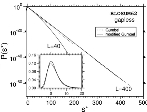
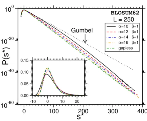
The main result is that most of the distributions we obtain deviate strongly from the Gumbel form, which is indicated in Fig. 7 and Fig. 8 by dotted lines. A typical example for the relative error of the results, obtained as explained above, is shown in Fig. 9. Note, that we used normalized scores s* = s - s0 by subtracting the position of the maximum s0 of the probability distribution. According to Eq. (3), the form of the Gumbel distribution is independent of the sequence length. In the limit L = M →∞. In practice this is not the case due to edge effects [17,18] and database applications use adjusted λ's, but the distribution is still assumed to be of Gumbel form. The results in this work suggest that this is only the case for not too small p-values.
One observes that the discrepancy seems to be stronger for shorter sequences. Also, the case without gaps (Fig. 8) deviates, at least for L = M = 400, only weakly from the Gumbel distribution. This might be expected due to the previous analytical work [9,10]. Qualitatively the behav-ior of the PAM250-matrices is the same and therefore the plots are not shown. A quantitative analysis of all results
( )
. . . . .
. . . .
wij =
1 0 6850 0 5017 0 2717 0 0480 0 0015
0 6850 1 0 7857 0 4624 0 00984 0 0034
0 5017 0 7857 1 0 6409 0 1607 0 0117
0 2717 0 4624 0 64
.
. . . . .
. . . 009 1 0 3587 0 0549
0 0480 0 0984 0 1607 0 3587 1 0 3777
0 0015 0 003
. .
. . . . .
. . 44 0 0117 0 3777 0 3777. . . 1 .
Relative error of the probability estimation using gapped sequence alignment and BLOSUM62 matrices
Figure 9
Relative error of the probability estimation using gapped sequence alignment and BLOSUM62 matrices.
0 100 200 300 400 500
s*
0.01001.0000
ε
(s*)
BLOSUM62 (12,1)
L=M=40
L=M=400
Probability distribution P(s) for ungapped sequence alignment using BLOSUM62-matrices
Figure 8
Probability distribution P(s) for ungapped sequence alignment using BLOSUM62-matrices. Deviations form the Gumbel-dis-tribution can only be observed for short sequences (L < 250). The inset shows the same data with linear ordinate.
0 100 200 300 400 500
s*
10-60 10-40 10-20 100
P(s*)
Gumbel modified Gumbel
0 10 20 0.00
0.04 0.08 0.12 0.16
Gumbel modified Gumbel
BLOSUM62
gapless
L=40
L=400
Probability distribution P(s) for gapped sequence alignment using BLOSUM62 matrices and affine gap costs with α= 12,
β= 1 for two sequences lengths L = M = 40 Figure 7
Probability distribution P(s) for gapped sequence alignment using BLOSUM62 matrices and affine gap costs with α= 12, β= 1 for two sequences lengths L = M = 40. The results for other lengths are summarized in additional file 1. Strong devi-ations from the Gumbel distribution become visible in the tail. The dotted lines show the original Gumbel distribution, when fitted to the region of high probability. The inset shows the same data with linear ordinate.
0 100 200 300 400 500
s*
10-7010-56 10-42 10-28 10-14 100
P(s*)
Gumbel Modified Gumbel
-5 0 5 10 15 20 0.00
0.05 0.10 0.15
Gumbel Modified Gumbel
BLOSUM62
(12,1)
L=M=40
will be given below. Empirically we find that the resulting distribution can be described by a modified Gumbel dis-tribution with a Gaussian correction:
with s0 = log(KLM)/λ. Note that we would have to use a dif-ferent normalization constant here, but since the correction dominates the tail of the distribution, the real normaliza-tion constant is numerically indistinguishable from λ. We modeled the data by a minimizing a weighted χ2 using the
program gnuplot [56]. The results including the reduced χ2
- values ( = χ2 /degrees of freedom) are documented in
Tab. 1 and as an additional CSV-file [see additional file 1].
All estimated standard errors in this paper are written behind the values and separated by "±".
Note that only for not too small sequences is in the order of one. This means that Eq. (18) describes the data better for longer sequences. However biological relevant sequence lengths (L > 200) sit in the range were the fit works fine. Moreover the results for shorter sequences are still several orders of magnitude below the naive Gumbel
result, which yield a value of about 104 for the L = 40
system.
We also tried smaller gap costs than α < 10 (β = 1, BLOSUM62) and α < 11 (β = 3, PAM250 matrices), but in this case the distributions deviate from Gumbel not only in the tail but even in the high-probability region. The reason is presumably that the values of the parameters are close to the critical value of the linear-logarithmic phase transition [24], i.e. the alignment is not really local any more.
Next, we study the scaling behavior of the correction parameter λ2. Since the distributions seem to approach the Gumbel distribution with increasing sequence length, as
P s( )=PGumbel( ) exps⋅ −λ2(s−s0)2 = λexp−λ(s−s0)−λ2(s−s0)2−e−−λ(s s−0),
(18) χ∗2
χ∗2
χ∗2
Table 1: Fit parameters of the modified Gumbel distribution Eq. (18) using the BLOSUM62 scoring matrix and affine gap costs with α
= 10, β= 1 . 104 describes the estimated value of λ
2 using the scaling relation Eq. (19). Fit parameters for other scoring systems
are provided as supplementary material to this artilce [see additional file 1].
L, M λ 104 λ
2 K S0 104
40 0.3272 ± 0.108% 8.6347 ± 0.412% 0.1028 ± 0.65% 15.597 ± 0.0676% 79.05 8.1560 ± 12.485% 60 0.3034 ± 0.086% 6.2007 ± 0.285% 0.0751 ± 0.60% 18.455 ± 0.0645% 49.40 6.1711 ± 12.907% 80 0.2892 ± 0.070% 4.8781 ± 0.222% 0.0612 ± 0.53% 20.644 ± 0.0540% 21.67 5.0458 ± 13.280% 100 0.2747 ± 0.072% 4.3187 ± 0.330% 0.0472 ± 0.58% 22.413 ± 0.0611% 39.42 4.3056 ± 13.627% 150 0.2541 ± 0.083% 3.2974 ± 0.529% 0.0303 ± 0.61% 25.682 ± 0.0422% 39.46 3.2047 ± 14.437% 200 0.2432 ± 0.063% 2.6343 ± 0.344% 0.0241 ± 0.52% 28.257 ± 0.0412% 10.47 2.5806 ± 15.214% 250 0.2359 ± 0.071% 2.1999 ± 0.454% 0.0198 ± 0.60% 30.196 ± 0.0459% 9.40 2.1701 ± 15.984% 300 0.2303 ± 0.061% 1.9101 ± 0.348% 0.0174 ± 0.54% 31.934 ± 0.0408% 2.00 1.8758 ± 16.758% 350 0.2261 ± 0.046% 1.6404 ± 0.239% 0.0153 ± 0.41% 33.334 ± 0.0300% 1.27 1.6525 ± 17.544% 400 0.2224 ± 0.052% 1.4806 ± 0.266% 0.0136 ± 0.49% 34.556 ± 0.0369% 1.36 1.4762 ± 18.347% 600 0.2140 ± 0.062% 1.0206 ± 0.384% 0.0106 ± 0.64% 38.561 ± 0.0472% 2.15 1.0250 ± 21.787% 800 0.2090 ± 0.063% 0.7660 ± 0.419% 0.0088 ± 0.67% 41.320 ± 0.0457% 1.82 0.7691 ± 25.697%
λ2extra
χ∗2
λ2extra
Probability distributions P(s) comparing different gap costs Figure 10
Probability distributions P(s) comparing different gap costs. The dotted line denote the distribution without Gaussian correction (λ2 = 0). Deviations from the Gumbel distribution
become stronger for small gap costs. The inset shows the same data with linear ordinate.
0 100 200 300 400
s*
10-6010-40 10-20 100
P(s*)
α=10 β=1
α=12 β=1
α=14 β=1
α=16 β=1
gapless
-10 0 10 20 0.00
0.05 0.10 0.15
BLOSUM62
can be seen in Fig. 7 and Fig. 8, we expect that λ2 decreases for L →∞. Furthermore, when looking at Fig. 10, where P (s) is shown for one sequence length L = M = 250 but for different gap-opening costs α, we expect a weak depend-ence of λ2 on α. In order to provide more quantitative evi-dence, we fitted all distributions by Eq. (18) and compared the resulting fit parameters.
In the gapless case no deviations from Gumbel could be detected for sequence lengths L > 200. For the other cases, the dependence of the scaling behavior λ2 on the sequence length is plotted in Fig. 11 and Fig.12. BLOSUM62 and PAM250 behaves qualitatively the same. λ2 seems to decay with a power law
for the smallest gap costs and faster than a power law for larger gap costs.
By fitting the limiting cases (two smallest gap costs) to this function an upper bound of the decay could be estimated. The results are summarized in Table 2.
Note that these arguments are purely heuristical attempts to look at the scaling behaviour and its upper bound. It is hard to decide, wether the extrapolation is valid for L = M
→∞. However an important range of biological
interesst-ing sequence lengths are governed with this scalinteresst-ing analy-sis.
In order to see the relevance of our result we consider a sim-ple examsim-ple, the E-value of a pair of sequences of length L = 100 using α = 12, β = 1 gap costs, the BLOSUM62-matrix and the SWISSPROT database [57], which contains cur-rently Nswissprot = 210, 623 sequences. In BLAST [58], the E-value, i.e. the expected number of hits exhibiting at certain "cut-off" score bcut, is currently estimated via the cumulative Gumbel distribution
λ2( )L =a L−b−λ2∗ (19)
E=KLN e⋅ −λbcut, (20)
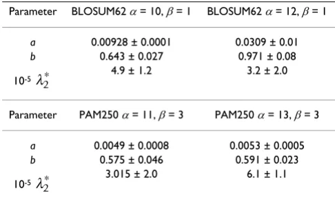
Table 2: Fitting parameters of the scaling relation Eq. (19).
Parameter BLOSUM62 α= 10, β= 1 BLOSUM62 α= 12, β= 1
a 0.00928 ± 0.0001 0.0309 ± 0.01
b 0.643 ± 0.027 0.971 ± 0.08
10-5 4.9 ± 1.2 3.2 ± 2.0
Parameter PAM250 α= 11, β= 3 PAM250 α= 13, β= 3
a 0.0049 ± 0.0008 0.0053 ± 0.0005
b 0.575 ± 0.046 0.591 ± 0.023
10-5 3.015 ± 2.0 6.1 ± 1.1
λ2∗
λ2∗
Scaling of the correction parameter λ2 (BLOSUM62) Figure 11
Scaling of the correction parameter λ2 (BLOSUM62). The decay of λ2 with system size shows approximately a power law near the logarithm-linear transition (two smallest gap costs). For this cases the fit to Eq. (19) is shown by a line (α = 10) and dots (α= 12). The lines of the remaining cases are guides to the eye conneting the data points.
40 60 80 100 150 200 300 400 600 800
L
10-5 10-4 10-3
λ
2α=10 β=1 α=12 β=1 α=14 β=1 α=16 β=1 gapless
BLOSUM62
Scaling of the correction parameter λ2 (PAM250) Figure 12
Scaling of the correction parameter λ2 (PAM250). The decay of λ2 with system size shows approximately a power law near
the logarithm-linear transition (two smallest gap costs). For this cases the fit to Eq. (19) is shown by a line (α= 11) and dots (α= 13). The lines of the remaining cases are guides to the eye conneting the data points.
40 60 80 100100 150 200 300 400
L
10-5 10-4 10-3
λ
2 α=11 β=3α=13 β=3
α=15 β=3
α=17 β=3 gapless
where L is the query length and N the total number of amino acids of the entire database, with parameters K = 0.0410 and λ = 0.267. Using the suggested E-value of 10 [58], we find a cut-off of bcut = 64.8 above which a result is considered to be significant, with [S > bcut] = 4.75 × 10⁻⁵.
Our cumulative distribution achieves this probability at bcut = 54, i.e. significantly below the BLAST value. Hence, using the true distributions of the scores, a considerable amount of queries, those which have a score between 54 and 64, are significant in contrast to the result of the significance esti-mation within the Gumbel approxiesti-mation. Hence, using the data provided in this work, one is able to estimate the significance of protein-data-base queries for the most com-monly used parameter sets with much higher precission than when applying the approximation of the Gumbel dis-tribution.
Sum statistics of the k-best alignments
The asymptotic distribution of the ungapped sum statistics is well known by Eq. (5). Again, we are interested in the dis-tributions for finite sequence lengths. We use the SIM pro-cedure [27] to compute the sum of the k-best alignments (k = 2, ..., 5) within the same type of Markov-chain Monte Carlo simulation as in the previous sections. In this case, we consider only the BLOSUM62 matrix together with affine gap costs α = 12, β = 1, a commonly used scoring system. We observed large fluctuations for short sequences (L < 100) and equilibration turned out to be harder for this case. Thus only sequences with L ≥ 60 (k = 2) and L ≥ 80 (k ≥ 3) have been used for the analysis. The temperature sets varied between {2.75, 3.0, 3.5, 4.0, 7.0, ∞} for L = 100, k = 2 and {6.25, 6.5, 7, 9, 11, ∞} for L = 400, k = 5 (details are shown in Tab. 3).
Note that for k > 3 the systems could not be equilibrated in the very low temperature regime T < 5. Therefore, for theses cases, the tail could only be obtained in an interme-diate range of probabilities (~10-20), which is nevertheless
low enough to obtain significance figures much better compared to using a simple-sampling approach.
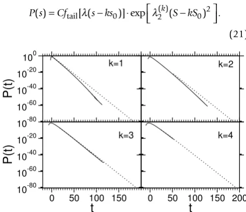
In Fig. 13 we compare different distributions obtained for varying k and fixed sequence length L = 200. Similar to the case of optimal alignment quadratic deviations could be observed which decrease with growing system length for all values of k (not shown).
In order to quantitatively compare the distribution with theoretical predictions from Karlin-Altschul statistics [28], we used the estimated Gumbel parameters λ and s0 from the optimal score distributions. Corresponding to substi-tuting the normalized score in Eq. (6) with t = λ (s - ks0)
we fitted the tail (p < 10-10) of the Monte Carlo data to the
modified distribution of the sum statistics, where the functional form ftail from Eq. (6) is again modified by a Gaussian factor:
P s( )=Cf [ (s−ks )] exp⋅ ( )k(S kS− ) .
tail λ 0 λ2 0 2
(21)
Score probability distributions for sum-statistics of the k-best scores (solid lines) for L = M = 200
Figure 13
Score probability distributions for sum-statistics of the k-best scores (solid lines) for L = M = 200. The dotted lines denote the distribution without Gaussian correction (λ2 = 0).
Devia-tions from Eq. (3) or Eq. (6) become only visible in the rare-event tail.
10-80 10-60 10-40 10-20 100
P(t)
0 50 100 150
t
10-80 10-60 10-40 10-20
P(t)
0 50 100 150 200
t
k=2
k=3 k=1
k=4
Table 3: Temperature parameters for sum-statistics.
L k = 2 k = 3 k = 4 k = 5
40 2.75, 3, 3.5, 4, 7, ∞ 60 2.75, 3, 3.5, 4, 7, ∞
80 2.75, 3, 3.5, 4, 7, ∞ 3.75, 4, 4.5, 5, 8, ∞ 5.25, 5.5, 6, 8, ∞ 6, 6.25, 6.5, 7, 8, 12, ∞ 100 2.75, 3, 3.5, 4, 7, ∞ 3.75, 4, 4.5, 5, 8, ∞ 5.25, 5.5, 6, 8, ∞ 6, 6.25, 6.5, 7, 8, 12, ∞ 150 2.75, 3, 3.5, 4, 7, ∞ 3.75, 4, 4.5, 5, 8, ∞ 5.25, 5.5, 6, 8, ∞ 6, 6.25, 6.5, 7, 8, 12, ∞ 200 3.25.3.5, 4, 7, ∞ 3.75, 4, 4.25, 4.5, 5, 8, ∞ 4.75, 5, 5.25, 5.5, 6, 8, ∞ 5.75, 6, 6.25, 6.5, 7, 8, 12,∞ 300 3.25.3.5, 4, 7, ∞ 3.75, 4, 4.25, 4.5, 5, 8, ∞ 4.75, 5, 5.25, 5.5, 6, 8, ∞ 5.75, 6, 6.25, 6.5, 7, 8, 12,∞ 400 3.25.3.5, 3.75, 4, 4.25, 5,
8,∞
This was possible for k = 2 and k = 3. The results are
sum-marized in Tab. 4 and the scaling behaviour of is
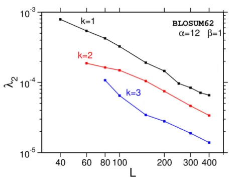
shown in Fig. 14. As in the case of the optimal score (k = 1), deviations from the theoretical form are significant only in the regime of small probabilities, which is not accessible with naive sampling methods. The data for k = 1 to k = 3 (Fig. 14) give evidence that the edge effect is reduced by increasing k. Note that in Ref. [16], best agreement with theory was achieved with k = 6.
Discussion and summary
We have studied the distribution of optimum alignment scores over a wide range using a rare-event sampling method. First, by comparing the results for a small 4-letter test system, we illustrated how the method works and pro-vided some evidence for its convergence. In the main part, we considered protein alignment for two types of substitu-tion matrices, i.e. BLOSUM and PAM matrices. We also
studied many different sets of biologically relevant param-eters by varying gap costs and sequence lengths.
For large enough gap costs it was previously assumed that the distribution follows the Gumbel extreme-value distri-bution, even when aligning finite sequences and allowing for gaps. Hence, the Gumbel distribution is used for calcu-lating p-values in protein data bases so far. We observe clear deviations from the Gumbel distribution in the biologi-cally relevant rare-event-tail, which is out of reach of simple sampling methods used so far.
An analysis of the scaling behavior of the correction param-eter λ2 gives evidence that the Gumbel distribution cor-rectly describes the data only in the limit of infinite sequence lengths, even for gapped sequence alignments. For finite protein lengths of biological relevance, we observed that the distributions can be fitted well by a Gum-bel distribution with a Gaussian correction. Therefore, for data bases like BLAST [8,18,58], we recommend to use dis-tribution functions determined by the empirical fitting parameters provided in this work because the critical value Scut, above which a result is considered to be significant, changes considerably, as we have seen.
We have also studied the sum-statistics of the k-best align-ments. Again a Gaussian correction to the assumed form of the distribution was found empirically. Extrapolation to infinitely long sequences gives good evidence that the ungapped statistical theory describes the gapped case for L = M →∞ as well.
λ2 ( )k
Scaling of the correction parameter for BLOSUM62 sum-sta-tistics (k = 1, 2, 3)
Figure 14
Scaling of the correction parameter for BLOSUM62 sum-sta-tistics (k = 1, 2, 3). λ2 is estimated by a fit for Eq. (21) using
optimal the Gumbel-parameters λand S0 from optimal score
statistics (k = 1).
40 60 80 100 200 300 400
L
10-5 10-4 10-3
λ
2BLOSUM62
α=12 β=1 k=1
k=2
k=3
Table 4: Correction parameter λ2 for the sum statistics k = 2 and k = 3. λ2 is estimated by a fit for Eq. (21) using optimal the Gumbel-parameters λand S0 from optimal score statistics (k = 1). BLOSUM62 with affine gap costs (α= 12, β= 1) was used as scoring system.
L
104 104
60 2.692 ± 0.30%
80 1.631 ± 0.63% 1.074 ± 2.59%
100 1.488 ± 0.23% 0.649 ± 2.06%
150 1.056 ± 0.06% 0.344 ± 1.90%
200 0.749 ± 0.13% 0.280 ± 1.14%
300 0.463 ± 0.15% 0.189 ± 0.70%
400 0.338 ± 0.29% 0.139 ± 0.92%
λ2 2 (k= )
Additional material
Acknowledgements
We thank B. Morgenstern and P. Müller for critically reading the manuscript. The authors have received financial support from the VolkswagenStiftung (Germany) within the program "Nachwuchsgruppen an Uni-versitäten", and from the European Community via the DYGLAGEMEM program.
References
1. Brown S: Bioinformatics Natick (MA): Eaton Publishing; 2000. 2. Rashidi S, Buehler L: Bioinformatics Basics Boca Raton (FL): CRC Press;
2000.
3. The Protein Data Bank [http://www.pdb.org.]
4. Fraser C, Gocayne J: The Minimal Gene Complement of Myco-plasma Genitalium. Science 1995, 270:397.
5. Needleman SB, Wunsch CD: A General Method Applicabel to Search for Similarities in the Amino Acid Sequence of two Proteins. J Mol Biol 1970, 48:443-453.
6. Smith TF, Waterman MS: Identification of Common Molecular Subsequences. J Mol Biol 1981, 147:195-197.
7. Gotoh O: An Improved Algorithm for Matching Biological Sequences. J Mol Biol 1982, 162:705.
8. Altschul S, Gish W, Miller W, Myers E, Lipman D: Basic Local Align-ment Search Tool. J Mol Biol 1990, 215:403-410.
9. Karlin S, Altschul S: Methods for assessing the statistical signifi-cance of molecular sequence features by using general scoring schemes. Proc Natl Acad Sci USA 1990, 87:2264.
10. Dembo A, Karlin S, Zeitouni O: Limit Distribution of Maximal Non-Aligned Two-Sequence Segmental Score. Ann Prob 1994, 22:2022-2039.
11. Yu Y, Hwa T: Statistical Significance of Probabilistic Sequence Alignment and Related Local Hidden Markov Models. J Comp Biol 2001, 8(3):249-282.
12. Yu Y, Bundschuh R, Hwa T: Statistical Significance and Extreme Ensemble of Gapped Local Hybrid Alignment. In Biological Evo-lution and Stati