doi:10.5194/tc-6-353-2012
© Author(s) 2012. CC Attribution 3.0 License.
Near-surface climate and surface energy budget of Larsen C ice
shelf, Antarctic Peninsula
P. Kuipers Munneke1, M. R. van den Broeke1, J. C. King2, T. Gray2, and C. H. Reijmer1
1Institute for Marine and Atmospheric Research, Utrecht University, Utrecht, The Netherlands 2British Antarctic Survey, National Environmental Research Council, Cambridge, UK Correspondence to: P. Kuipers Munneke (p.kuipersmunneke@uu.nl)
Received: 20 September 2011 – Published in The Cryosphere Discuss.: 12 October 2011 Revised: 12 March 2012 – Accepted: 18 March 2012 – Published: 27 March 2012
Abstract. Data collected by two automatic weather stations (AWS) on the Larsen C ice shelf, Antarctica, between 22 Jan-uary 2009 and 1 FebrJan-uary 2011 are analyzed and used as input for a model that computes the surface energy budget (SEB), which includes melt energy. The two AWSs are sep-arated by about 70 km in the north–south direction, and both the near-surface meteorology and the SEB show similarities, although small differences in all components (most notably the melt flux) can be seen. The impact of subsurface absorp-tion of shortwave radiaabsorp-tion on melt and snow temperature is significant, and discussed. In winter, longwave cooling of the surface is entirely compensated by a downward turbulent transport of sensible heat. In summer, the positive net radia-tive flux is compensated by melt, and quite frequently by up-ward turbulent diffusion of heat and moisture, leading to sub-limation and weak convection over the ice shelf. The month of November 2010 is highlighted, when strong westerly flow over the Antarctic Peninsula led to a dry and warm f¨ohn wind over the ice shelf, resulting in warm and sunny conditions. Under these conditions the increase in shortwave and sensi-ble heat fluxes is larger than the decrease of net longwave and latent heat fluxes, providing energy for significant melt.
1 Introduction
Over the past 50 yr, the Antarctic Peninsula has seen an atmo-spheric warming that is much larger than the global average (Turner et al., 2005). In relation to this, Antarctic Peninsula ice shelves, which are the floating extensions of glaciers orig-inating in the mountains of the Antarctic Peninsula, have re-treated everywhere in this region (Cook and Vaughan, 2010). The collapse of Larsen A and B ice shelves (Rott et al., 1996) have become iconic images for the rapid climate change in
this region. The disappearance of ice shelves has caused acceleration and thinning of the glaciers previously feeding them (Rignot et al., 2004; Scambos et al., 2004; Rott et al., 2011). Whether the shrinkage of the ice shelves is driven mainly by atmospheric warming or by changes in oceanic cir-culation underneath is a subject of scientific discourse, but it is certain that atmospheric warming has profound effects on the state of the snow and firn layer covering the ice shelves (Holland et al., 2011). It has been hypothesized that an in-crease in snowmelt could enhance hydrofracturing of surface crevasses (Scambos et al., 2000; Van den Broeke, 2005), in-fluencing the stability of ice shelves.
Fig. 1. Map of the Antarctic Peninsula central section. UU/IMAU
AWS network locations shown in green; partner AWS network shown in orange; Rothera Research Station shown in blue.
2 Data and methods
The data collected by the two AWSs described in this paper are used to drive a model that calculates the surface energy budget. In this section, we describe the AWS sites, their in-strumentation, the way in which we corrected the raw data, and we briefly discuss the surface energy budget model. 2.1 AWS sites and instrumentation
AWS 14 is the northerly UU/IMAU AWS at 67◦00.80S 61◦28.80W (see map in Fig. 1), at an elevation of 40 m a.s.l. The other station, AWS 15, is located about 70 km to the SSW at 67◦34.30S 62◦07.50W (also at 40 m a.s.l). Both sta-tions are situated roughly 125 km from the grounding line to the west, and 55 km from the ice shelf front to the east. The stations are equipped with a GPS antenna, data from which indicate that both stations are moving eastward by about 400 m yr−1. The surface at both locations is homogeneous
and flat, with a surface slope less than 0.1◦. The stations were installed in January 2009, serviced in January 2010, and ser-viced and raised in January 2011.
The following quantities are measured by both AWSs: air temperature (Ta) and relative humidity (RH) by a Vaisala
HMP35AC. The temperature sensor is naturally-ventilated. Air pressure (p) is measured by a Vaisala PTB101B. Wind speed (v) and direction are observed using a Young 05103, and the radiative fluxes (shortwave fluxes, SW↓ and
SW↑; longwave fluxes, LW↓ and LW↑) are measured by
a naturally-ventilated Kipp and Zonen CNR1 radiometer. The tilt of the AWS mast in two perpendicular directions is observed using homemade inclinometers, and snow temper-ature (Tsn) is measured by thermistor strings at initial depths
Table 1. Means of meteorological variables 1 February 2009–
31 January 2011 (28 January 2011 for AWS 15). ANN=average over all months.
AWS 14 ANN DJF MAM JJA SON
Air temperature (2 m) ◦C −15.5 −4.2 −20.1 −24.0 −13.4 Specific humidity (2 m) g kg−1 1.33 2.52 0.84 0.60 1.41 Relative humidity (2 m) % 94.8 90.6 98.9 96.3 93.3 Surface temperature ◦C −16.1 −4.0 −20.7 −25.2 −14.2
Wind speed m s−1 4.5 4.4 3.9 4.3 5.4
Air pressure hPa 985.1 986.4 985.5 988.7 979.8
AWS 15 ANN DJF MAM JJA SON
Air temperature (2 m) ◦C −15.8 −4.5 −20.2 −24.0 −13.7 Specific humidity (2 m) g kg−1 1.30 2.49 0.82 0.60 1.36 Relative humidity (2 m) % 94.7 90.9 98.0 96.3 93.3 Surface temperature ◦C −16.7 −4.6 −21.0 −25.4 −14.8
Wind speed m s−1 4.3 4.5 3.6 4.0 5.0
Air pressure hPa 985.1 986.7 985.5 988.5 979.7
of 0.25, 0.50, 1.0, 2.0, 3.0, 4.0, 5.0, 7.0, 10.0, and 15.0 m. During the 2011 visit, new snow thermistors were installed at 0.05, 0.10, 0.20, 0.40, and 0.80 m depth. To minimize so-lar loading, the thermistor strings were placed inside a white plastic cover. Additionally, surface height is measured using a sonic height ranger. The initial height of the wind and air temperature sensors was 3.80 m above the snow. All quanti-ties are sampled every 6 min, from which hourly means are stored on a Campbell CR10X datalogger. An exception to this is the air pressure, which is sampled once per hour. 2.2 AWS data treatment
Data coverage of AWS 14 is continuous between 20 Jan-uary 2009 and 1 April 2011. Hourly data were recovered from the data logger on 16 January 2011, and data between 16 January and 1 April 2011 have been received from the ARGOS satellite network. As the ARGOS data transmission fails occasionally, data are temporally interpolated when no data are available for a particular hour. Data coverage of AWS 15 is also continuous between 20 January 2009 and 28 January 2011. Since then, the ARGOS antenna malfunc-tioned, so that no data are available after that date.
-50 -40 -30 -20 -10 0
AWS 14
AWS 15
2
m
Ai
r
T
e
mp
.
(
oC)
0 5 10 15
Jan/1/09 Sep/1/09 May/1/10 Jan/1/11
1
0
m
W
in
d
Sp
e
e
d
(m
s
-1) 0 1 2 3
2
m
Sp
e
c.
h
u
m.
(g
kg
-1)
9.5 104 9.7 104 9.9 104 1.01 105
Ai
r
p
re
ssu
re
(Pa
)
Fig. 2. Daily-averaged air temperature, specific humidity, air
pres-sure, and wind speed for the measurement period. AWS 14 data are shown in black with circles, AWS 15 is shown in red.
Relative humidity is corrected with respect to sublimation over ice. Since the air temperature screen is not ventilated to save energy, an overestimation of air temperature occurs on calm, sunny days. A correction is applied that is a func-tion of wind speed and the sum of the incoming and reflected shortwave fluxes (Smeets, 2006).
2.3 Surface energy budget model
The SEB model used in this study is identical to the one used in Kuipers Munneke et al. (2009), including the computa-tion of subsurface absorpcomputa-tion of solar radiacomputa-tion. For details, we refer to the above-mentioned paper, but we will reiter-ate the concept of the model here. The model usesp, RH,
Ta, v, SW↓, SW↑, and LW↓ as input. The sensible heat
fluxHsenand latent heat fluxHlatare calculated using a bulk
method, applied to the air layer between the sensor level and the snow surface. The ground heat fluxGis calculated using
Fig. 3. Measured density profiles between 0 and 0.60 m depth below
the surface. The black line is the mean and the grey area represents one standard deviation of 60 density profiles measured between 16 and 28 January 2011.
a multi-layer snowpack that allows for melting, refreezing, and percolation of meltwater. The SEB equation is:
SW↓+SW↑+Q+LW↓+LW↑+Hsen+Hlat+G=M, (1)
whereM is the sum of of surface and subsurface melt. Q
is the amount of shortwave radiation absorbed below the sur-face. All fluxes are defined as positive when directed towards the surface. In previous studies, an expression like Eq. (1) describes the energy budget of an infinitesimally small skin layer. Here, we take into account radiation in the subsur-face, and therefore all the terms in Eq. (1) apply to the entire snowpack. Thus, M is the sum of surface and subsurface melt, andGis computed as the rate of change in heat content of the entire snowpack (see Kuipers Munneke et al., 2009).
In the left-hand side of Eq. (1), LW↑,Hsen, Hlat, andG
are more or less directly a function of the surface (or: skin) temperature. In an iterative procedure, this skin temperature is found for which all the terms in Eq. (1) add up to zero. The solution for the skin temperature that we find in this way is unique. A verification of LW↑, that is computed from the
re-trieved skin temperature, against the observed LW↑provides
a means to assess the performance of the SEB model. In this way, a closed, consistent, and testable surface energy budget is found.
Fig. 4. Wind roses of daily mean wind speed and direction for the
period 1 February 2009–31 January 2011, for AWS 14 (left) and 15 (right). The percentages refer to the frequency of occurence.
we explore other settings of this variable, and discuss its appropriateness.
The model snow density profile for both AWSs is derived from the mean of more than 60 snow pits dug in January 2011 around AWS 14, and taken constant over the entire period. The error associated with this assumption is small (Van As et al., 2005; Kuipers Munneke et al., 2009). The mean snow density profile from the 60 snow pits is shown in Fig. 3. The density increases with depth for the first 0.25 m, likely due to the fact that the snow layers around that depth are older and underwent multiple melt and refreeze cycles during the melting season that had started already two months before the snow pits were dug.
The temperature of the model snowpack is initialized us-ing thermistor strus-ing observation at the start of the observa-tion period.
3 Results
First, we will discuss the general near-surface meteorological conditions in Sect. 3.1. In Sect. 3.2, we present the different components of the SEB. In Sects. 3.3–3.5, we zoom in on some particular aspects of the SEB and their relation to the near-surface meteorology on Larsen C ice shelf.
3.1 Near-surface meteorology
Here, we give an overview of the near-surface meteorology of both AWS sites for the measurement period. Due to the short period under consideration, this overview should not be seen as a site climatology, but rather as a description of the typical meteorological conditions encountered during these two years. Since the sensor height above the surface is changing due to snow accumulation, we interpolate air tem-perature and humidity to the 2-m level using vertical profiles that emerge from the bulk method for turbulent fluxes de-scribed above. Likewise, wind speed is extrapolated to 10 m above the surface.
0 4 8 12 16
2009 2009.5 2010 2010.5 2011
C
lo
u
d
o
p
ti
ca
l t
h
ickn
e
ss AWS 15
AWS 14
Fig. 5. Monthly means of cloud optical thickness (see text) at
AWS 14 (black) and 15 (red).
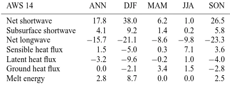
Table 2. Means of SEB components 1 February 2009–31
Jan-uary 2011 for AWS 14, in W m−2. ANN=average over all months.
AWS 14 ANN DJF MAM JJA SON
Net shortwave 17.8 38.0 6.2 1.0 26.5
Subsurface shortwave 4.1 9.2 1.4 0.2 5.8
Net longwave −15.7 −21.1 −8.6 −9.8 −23.3
Sensible heat flux 1.5 −5.0 0.3 7.1 3.6
Latent heat flux −3.2 −9.6 −0.2 1.0 −4.0
Ground heat flux 0.0 −2.1 3.4 1.5 −2.8
Melt energy 2.8 8.7 0.0 0.0 2.5
The mean 2-m (nominal) air temperature at AWS 14 (15) is−15.5 (−15.8)◦C (see Table 1 and Fig. 2). In summer, the melting surface keeps the air temperature close to 0◦C, and the temporal variability is reduced. From autumn to spring, temperature variability is much larger, as the air tempera-ture is governed mainly by advection. During advection of warm air, near-surface temperature can rise close to the melt-ing point even in winter, like on 14 July 2010 (−0.6◦C at AWS 14) or 13 September 2010 (1.5◦C). The lowest tem-perature recorded during this period was−46.9 (−45.4)◦C
at AWS 14 (15) on 12 (10) July 2009.
Specific humidity exhibits a strong annual cycle, with one order of magnitude higher values during the summer months. In general, the air over the Larsen C ice shelf is very moist, with a mean relative humidity of almost 95 % at both stations (Table 1).
The mean wind speed is 4.5 (4.3) m s−1at AWS 14 (15)
-60 -40 -20 0
-60 -40 -20 0
Mo
d
e
le
d
su
rf
a
ce
t
e
mp
e
ra
tu
re
(
o C)
Observed surface temperature (oC) a) AWS 14
-60 -40 -20 0
-60 -40 -20 0
Observed surface temperature (oC) b) AWS 15
Fig. 6. Model performance check by comparing observed values of surface temperature to computed values, for (a) AWS 14; and (b) AWS 15.
Red dots are hourly values, whereas black dots are daily-mean values.
-40 -20 0 20 40 60
2009 2009.5 2010 2010.5 2011
En
e
rg
y
flu
x
(W
m
-2) Net shortwave
Net longwave
Sensible heat
Latent heat
Melt
Ground heat
(a) AWS 14
Subsurface shortwave
-40 -20 0 20 40 60
2009 2009.5 2010 2010.5 2011
En
e
rg
y
flu
x
(W
m
-2) Net shortwave
Net longwave
Sensible heat
Latent heat
Melt
Ground heat
(b) AWS 15
Subsurface shortwave
Fig. 7. Monthly means of surface energy budget components (in W m−2) for (a) AWS 14; and (b) AWS 15.
is the dominant wind direction at AWS 15, while at AWS 14 it is more SSW/SW. This turning of the wind results from cyclonic flow around a climatological low-pressure area over the Weddell Sea. The strongest winds also blow from these dominant directions, resulting from the above-mentioned cy-clonic flow in combination with the topographic constraint of the mountains to the west. The weakest winds are blowing from the NW and E at both stations.
We computed cloud optical thickness using an algorithm that relates the observed SW↓ to the theoretical clear-sky
value of SW↓ (Fitzpatrick et al., 2004), extrapolated to the
winter months using a good correlation between cloud opti-cal thickness and the longwave radiation balance in summer (Kuipers Munneke et al., 2010). The cloud cover at AWS 15 is generally optically thicker than at AWS 14 (Fig. 5). At both locations, cloud cover is optically thinnest in late winter and spring, when the atmosphere is coldest and sea-ice cover over the Weddell Sea reduces evaporation of sea water.
3.2 Surface energy budget
As explained above, the SEB model iteratively finds a skin temperature for which the energy budget is closed. The per-formance of the SEB model is tested by comparing this re-trieved skin temperature to the observed surface tempera-ture (computed with LW↑) (Fig. 6). Based on hourly (daily)
means, the difference is 0.44 (0.44) K for AWS 14, with a RMS difference of 1.40 (1.08) K. At AWS 15, the differ-ence based on hourly (daily) means is 0.19 (0.19) K, with a RMS difference of 1.48 (1.10) K.
Monthly mean values of all SEB components are pre-sented in Fig. 7 for both locations. Seasonal and annual averages of all SEB components are shown in Table 2. At both sites, there is a clear annual cycle in all the SEB compo-nents. In winter, SWnetvanishes (JJA: 1.0 W m−2). The
sur-face starts cooling, so that LW↑decreases and the net
260 265 270 275
Jan/17/2011 Jan/31/2011 Feb/14/2011 Feb/28/2011 Mar/14/2011 Mar/28/2011
T
e
mp
e
ra
tu
re
(K)
No radiation penetration
RP, 0.1 mm RP, 0.5 mm
Observed
Fig. 8. Comparison between observed and modeled snow
tem-perature at 0.5 m depth at AWS 14, for different model settings of radiation penetration. Observed snow temperature (interpolated to 0.5 m) shown in black; model without radiation penetration in green; model with radiation penetration (0.1 mm snow grain radius) in blue; model with radiation penetration (0.5 mm snow grain ra-dius) in red.
latent heat flux becomes small in winter (JJA: 1.0 W m−2), since the low air temperature reduces near-surface specific moisture gradients, inhibiting effective heat loss through sub-limation. In the winter of 2009, the sensible heat flux is also low or slightly positive, indicating that there is some vertical transport of warmer air towards the surface through turbu-lent motion. In the winter of 2010, the sensible heat flux attains higher values, which is caused by frequent advection of warmer air (see air temperature record in Fig. 2). This means that more heat is transported to the surface. The re-sulting increased surface temperature decreases the net long-wave radiation, restoring the surface energy balance.
In summer, net shortwave radiation is the most prominent source of energy – it is balanced by a net longwave cooling (DJF value:−21.1 W m−2), and by a negative latent heat flux (DJF:−9.6 W m−2) indicating a steady sublimation. More-over, a slightly negative sensible heat (DJF:−5.0 W m−2) is visible in summer, indicating that the surface layer becomes unstable and convective in nature. We will discuss this fea-ture in more detail in Sect. 3.4. The negative ground heat flux (DJF:−2.1 W m−2) indicates that the snowpack is heat-ing up. A considerable amount of energy is consumed by melting (DJF: 8.7 W m−2).
There are some small differences in the SEB of the two locations. First of all, the net shortwave radiation is some-what larger at AWS 14 (18 W m−2annually averaged) than
at AWS 15 (13 W m−2). This is caused by a somewhat higher
albedo at AWS 15 (0.88 averaged over the entire period com-pared to 0.85 at AWS 14). The higher albedo is caused by the thicker cloud cover, which in itself also is a cause for reduced incoming shortwave radiation. The mean transmis-sivity of the atmosphere (including clouds) for shortwave ra-diation is slightly smaller at AWS 15 than at AWS 14, due to the thicker cloud cover. If we apply the transmissivity of
0 20 40 60 80 100
Jan/4/2011 Jan/8/2011 Jan/12/2011 Jan/16/2011 Observed height change
Total melt = surface + subsurface melt
Surface melt
Subsurface melt
C
u
mu
la
ti
ve
me
lt
/
h
e
ig
h
t
ch
a
n
g
e
(mm)
RP, 0.1 mm
RP, 0.5 mm
No radiation penetration
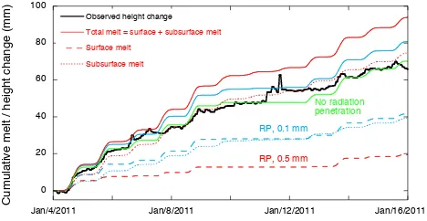
Fig. 9. Comparison of observed cumulative height change and
mod-eled cumulative melt at AWS 14, for different model settings of radiation penetration. Observed height change (converted to mm w.e. assuming a density of 400 kg m−3) shown in black; model without radiation penetration in green; model with radiation pen-etration (0.1 mm snow grain radius) in blue; model with radiation penetration (0.5 mm snow grain radius) in red. Dotted lines indicate subsurface melt; dashed lines indicate surface melt; and solid lines indicate total melt (=surface+subsurface melt).
AWS 14 to SW↓from AWS 15, we find that the direct effect
of the thicker cloud cover on SWnet is small (0.6 W m−2),
and that the remaining difference in SWnetof these locations
is due to a differing albedo.
In a relative sense, the largest difference between the two locations is the melt flux: averaged over the year, the melt energy flux at AWS 14 is more than twice that at AWS 15. However, it is important to note that the melt flux is a sum of large terms of opposite sign, so that this difference may be of the same order of magnitude as the uncertainty of the melt flux. Independent estimates of the melt rate over the Larsen C ice shelf suggest a smaller difference between the two locations (Kuipers Munneke et al., 2012). The lower net radiative flux at AWS 15 results in slightly less negative ground and latent heat fluxes in summer.
For filling wind data gaps due to riming of the wind sen-sor, we have assumed a constant wind speed of 1 m s−1, a value that could also have been chosen different. This has an impact on the modelled fluxes. When we use a very high constant value of 5 m s−1, the sensible heat flux
increases most notably, by a factor of 2–3. As the wind data gaps are at most a few days, monthly-mean fluxes are only marginally affected: all monthly-mean fluxes change by less than 1 W m−2. The modelled surface temperature of June 2009, a month with 5 days of missing wind data, is 0.1◦C higher when we use 1 m s−1 than when we use 5 m s−1.
-50 0 50 100 150
19-Jan-2011 20-Jan-2011 21-Jan-2011 22-Jan-2011 23-Jan-2011
En
e
rg
y
flu
x
(W
m
-2)
Net shortwave
Net longwave
Melt
Sensible heat Latent heat
Ground heat
Subsurface shortwave
-10 -5 0 5
T
e
mp
e
ra
tu
re
(
oC
);
W
in
d
sp
e
e
d
(m
s
-1)
Wind speed
Surface temperature
2-m temperature
Fig. 10. Meteorological conditions (upper panel) and selected SEB components (lower panel) during a four-day period showing typical
daytime convection.
on the SEB and near-surface meteorology, we give special attention to this period in Sect. 3.5.
3.3 Radiation penetration, snow temperature, and melt
The role of shortwave radiation penetration in the snowpack is to deliver energy below the surface, enabling a more rapid transfer of energy into the snow (Brandt and Warren, 1993; Kuipers Munneke et al., 2009). Shortwave radiation penetra-tion depends on the size of the snow grains: the larger the grains, the more photons are scattered in the forward direc-tion (i.e. into the snowpack), leading to more absorpdirec-tion of shortwave radiation inside the snowpack. Inclusion of this process into the SEB has two important consequences: first, the uppermost snow layers heat up more quickly in summer. Second, the absorption of shortwave radiation in layers be-low the surface albe-lows for a larger contribution of subsurface melting. The partitioning of melt into surface melt and sub-surface melt will change when shortwave radiation penetra-tion is allowed. Moreover, when the snowpack is near or at the melting point, the total melt (the sum of surface and sub-surface melt) increases.
0 200 400 600 800 1000 1200
270 271 272
H
e
ig
h
t
a
b
o
ve
su
rf
a
ce
(m)
! (K) 22 Jan 2011 15.19 LT = 18.19 UTC
Fig. 11. Vertical profile of potential temperature (in K) from a
ra-diosonde launched on 22 January 2011 at 15:19 LT (=18:19 UTC). The horizontal dashed line indicates the height at which dθ/dz
changes sign, while the vertical dashed line illustrates that possi-ble convection extends up to 1150 m, the height at which potential temperature equals surface potential temperature.
The implication for the melt budget is clearly observed in Fig. 9. Without accounting for radiation penetration, the to-tal melt (green solid line) equals the surface melt, since sub-surface melt is zero. Radiation penetration leads to smaller surface melt (dashed lines), but the increase in subsurface melt (dotted lines) is larger than the decrease in surface melt, resulting in a net higher total melt (solid lines). We have attempted to corroborate these results with the sonic height ranger for the period 4–16 January 2011 (black line in Fig. 9), assuming a constant density of the melted snow of 400 kg m−3(as we do not really know which snow or ice lay-ers are melting). We found a reasonable agreement, although a discrepancy with modeled melt remains. The comparison is difficult since the sonic height ranger itself is not anchored to a fixed reference surface, nor is it known which part of the snowpack is actually melting (low-density surface snow or high-density subsurface snow and ice lenses). Moreover, the height change signal also includes densification and ac-cumulation. This has a large impact on the conversion from height change to a melt rate, and thus the melt signal derived from observations has quite a large uncertainty. Therefore, it cannot be concluded from the comparison in Fig. 9 which setting for radiation penetration is the most adequate to simu-late the SEB at this site. On the positive side, the comparison
Height of 850 hPa level (m)
Fig. 12. Surface wind speed and direction (vectors) and the height
of the 850 hPa level from RACMO2, for (a) 15 November 2010 and
(b) 19 November 2010. The location of AWS 14 is denoted with
the black dot.
shows that the model computes a melt signal that corresponds well to the observed height change, both in magnitude and in variability.
3.4 Convection and a ceasing temperature inversion
An interesting feature of the summertime SEB at both lo-cations is the frequent occurrence of a negative sensible heat flux. This indicates that the surface layer, normally character-ized by a temperature inversion in the polar regions, breaks down and gives way to convective turbulent motion. Con-vection occurs so frequently that the monthly-mean sensible heat flux becomes negative in the summer months (Fig. 7). We study this phenomenon in more detail in this section.
A typical Antarctic boundary layer is characterized by a stable stratification and a temperature deficit at the surface. In winter, this temperature deficit is driven by a radiation deficit at the surface. In response, sensible heat is transported towards the surface by turbulent motion in the atmosphere. In summer, a temperature inversion can still exist, but then it is usually limited to nighttime, or driven by advection of warm air over a melting surface, the temperature of which is limited to the melting point. This situation also leads to a sensible heat flux directed towards the surface.
-150 -100 -50 0 50 100 150 200 250
10 12 14 16 18 20 22 24 26
Net shortwave Net longwave Sensible heat Latent heat Melt
En
e
rg
y
fl
u
x
(W
m
-2)
November 2010
NW NW W SW W NW SE W E S E SE SE SW W
N
Fig. 13.
Selected SEB components between 10 and 26 November 2010. Daily-mean wind direction is
shown at the bottom of the panel.
34
Fig. 13. Selected SEB components between 10 and 26
Novem-ber 2010. Daily-mean wind direction is shown at the bottom of the panel.
2-m temperature by up to 2–3◦C. There is little wind, blow-ing from the S to E. This wind advects humid and cloudy air from the Weddell Sea: manual weather observations made during this period reveal a mean cloud cover of 7.7 oktas (n= 32) with a cloud base at 1–1.5 km above the surface. The cloud cover results in only a slightly negative net longwave flux, making the sum of net longwave and shortwave fluxes on the order of 50–70 W m−2. This radiative heating of the snow surface is compensated by melting and/or by upward turbulent fluxes of heat and moisture (sublimation). The ver-tical extent of this convective layer is determined when plot-ting a vertical profile of potential temperatureθ obtained by a radiosonde (Fig. 11). Negative values of dθ/dzare a sign of an unstable boundary layer, and extend up to only 50 m above the surface. Theoretically, an air parcel can be lifted to the level at which the potential temperature equals the sur-face potential temperature, which is at about 1150 m, which is the possible depth of convection.
3.5 November 2010: strong westerlies and intense melting
In the two-year time series discussed in this paper, Novem-ber 2010 stands out as a peculiar month, with low net long-wave radiation, high net shortlong-wave radiation, and signifi-cant melt occurring already in the austral spring. Using the regional atmospheric model RACMO2 at 27-km hori-zontal resolution (Lenaerts et al., 2012), which is forced at the lateral boundaries by ERA-Interim reanalysis data, we found persistent westerly winds flowing over the Antarctic Peninsula for a period of 15 days (2–18 November 2010).
Table 3. Means of SEB components and meteorological
vari-ables for the two contrasting periods 10–18 November, and 19– 25 November 2010 for AWS 14.
AWS 14 10–18 Nov 19–25 Nov
Air temperature (2 m) ◦C −0.4 −5.6 Relative humidity (2 m) % 79 92
Wind speed m s−1 6.0 5.6
Net shortwave 63.1 37.8
Subsurface shortwave 13.3 8.8
Net longwave −49.9 −25.0
Sensible heat flux W m−2 16.5 −6.8
Latent heat flux −13.0 −11.1
Ground heat flux −7.8 −3.2
Melt energy 29.6 0.9
Moderate westerlies impinging on the Antarctic Peninsula mountains have been shown to cause a northerly flow on the eastern side of the Peninsula (Orr et al., 2004), advecting warm air over the ice shelves. When the westerly flow be-comes even stronger, the air flows over the mountains, caus-ing a f¨ohn effect on their lee side. Under these conditions, the local meteorological conditions at Larsen C ice shelf are characterized by cloudless skies and a north-to-westerly ad-vection of dry and warm air.
To illustrate the effect of this warm northerly flow and westerly f¨ohn winds, we zoom in at the period 10–25 Novem-ber 2010. This period shows two very constrasting regimes: between 10 and 18 November, the flow was predominantly from the north and west; between 19 and 25 November, the wind was from the south and east. The near-surface wind and 850 hPa geopotential heights typical for these constrast-ing regimes are illustrated in Fig. 12. In Fig. 13, we show the SEB components at AWS 14 between 10 and 25 Novem-ber 2010, along with the observed daily mean wind direc-tion. Additionally, Table 3 shows the means of meteorolog-ical variables and SEB components for these two contrast-ing periods. In the first half of this period, strong west-erly flow west of the peninsula travels over the mountains onto the ice shelves. The descending motion east of the mountains warms and dries the air. The resulting clear-sky conditions are reflected in the SEB as low net longwave radiation (−49.9 W m−2), and high net shortwave radiation
(63.1 W m−2). Since the snow surface is at the melting point
during the day and the air temperature is above 0◦C, the
shortwave and sensible heat fluxes outweighs the decrease of the longwave and latent heat fluxes. As a result, a rel-atively large amount of energy is available for snow melt (29.6 W m−2).
From 19 November onwards, the atmospheric flow comes from the east and south, bringing cold and cloudy air in from the Weddell Sea and colder regions to the south. This is immediately reflected in the SEB: net shortwave fluxes are much smaller, and sensible heat fluxes are now negative (−6.8 W m−2), indicating weak convection over the ice shelf.
The negative sensible heat flux is explained by the advection of cold air over a warm and wet snowpack that first needs to refreeze before it can start to cool.
4 Conclusions
Two years of data collected by the two AWSs on Larsen C ice shelf offer a preliminary insight into the SEB typical for this region. The time series are too short to present a climatology, but several interesting aspects of the SEB can be highlighted. First of all, the importance of modelling subsurface ab-sorption of solar radiation and its implications on total melt have been discussed. However, it remains difficult to de-termine the best settings for this part of the model. Per-haps a seasonally varying density profile and snow grain size would improve the simulation of the snowpack. A radical step would be to incorporate snow densification and snow metamorphism into the SEB model, but we did not pursue this for the present study. Furthermore, it is important to stress that taking into account radiation penetration does not always lead to an increase in total melt like we showed in Fig. 9. For a cold snowpack for example, disregarding ra-diation penetration concentrates all absorbed solar rara-diation in the surface layer, which may cause melt to occur. When radiation penetration would be enabled, the absorbed solar radiation would be distributed over a certain depth so that none of the uppermost layers would experience melt. Thus, the observation that radiation penetration leads to more melt is true only for a snowpack at or very close to the melting point.
Also, we have shown that calm and cloudy conditions dominate in summer, and can give rise to long continuous periods of daytime surface melt, as well as daytime convec-tion in the surface layer. On quite a number of days in sum-mer, the air temperature at 2 m above the surface remains below 0◦C while the surface is melting. Interestingly, this
means that air temperature measured at some distance above the surface, is not necessarily a good indicator of melt. Mod-els or algorithms that depend solely on air temperature input for the computation of melt (like positive degree-day mod-els) will likely underestimate the amount of melt when the air temperature input is recorded well above the surface. This stresses the need not only to model the full SEB, but also to
measure the SEB with an AWS, including the individual ra-diation components.
Although the analysis is limited to only two locations, the topographic homogeneity makes that the results presented here are representative for a large area. Especially in the north-south direction, there are some notable climate gra-dients over Larsen C ice shelf, however: in several surface mass balance components (Lenaerts et al., 2012), in firn air conditions (Holland et al., 2011), and in number of melt days (Tedesco and Monaghan, 2009). These gradients are a result of gradients in the SEB components, and ultimately of gra-dients in meteorological variables like temperature and cloud cover. Already between AWS 14 and 15, separated by a mere 70 km, differences in melt and other SEB components can be seen. It would be interesting and useful to compare observa-tions from other locaobserva-tions to get insight in the spatial variabil-ity of near-surface climate and SEB. To that end, BAS and UU/IMAU extended the coverage of the Antarctic Peninsula ice shelves northward by installing an AWS at Scar Inlet, the remains of the Larsen B ice shelf (AWS 17, shown on the map in Fig. 1) in February 2011.
Lastly, we illustrated the important effect that westerly flow crossing the Antarctic Peninsula mountain range has on the SEB and most importantly on the melt flux. Over the past 50 yr, the Antarctic Peninsula has seen a large tempera-ture increase (Turner et al., 2005), linked to a positive trend of the Southern Annular Mode (SAM, the principal mode of variability in the atmospheric circulation of the Southern Hemisphere extratropics, Marshall, 2003). Given the marked increase in westerly flow during this period (Marshall, 2002), the melt volume has likely increased over these 50 yr. Since the late 1970s however, melt trends have been stagnant in the Antarctic Peninsula (Tedesco, 2009; Kuipers Munneke et al., 2012). The future trend of temperature and melt is uncer-tain, but continued observation and modelling is crucial to understand the repercussions of future climate change on the surface energy budget, and ultimately on the stability of the ice shelves in the Antarctic Peninsula.
Acknowledgements. We would like to thank Ian Hey, Ian Potten,
Nick Alford (BAS) and Wim Boot (IMAU) for help with instal-lation and maintenance of the two IMAU Automatic Weather Stations. Henk Snellen and Marcel Portanger are thanked for help with the development of the Automatic Weather Stations and data transfer. Phil Anderson (BAS) is thanked for his contribution in the 2011 field experiment at the AWS 14 site. This work was supported partly by funding from NWO/ALW grant 818.01.016, and partly by funding from the ice2sea programme from the European Union 7th Framework Programme, grant number 226375. Ice2sea contribution number 057. The radiosonde measurements presented in Fig. 11 were carried out as part of the project Orographic Flows and the Climate of the Antarctic Peninsula (OFCAP), funded by the UK Natural Environmental Research Council (NERC). Constructive reviews from R. Dadic and D. J. Lampkin have been very much appreciated, and helped to improve this paper.
References
Andreas, E. L.: A theory for the scalar roughness and the scalar transfer coefficients over snow and sea ice, Bound.-Lay. Meteo-rol., 38, 159–184, 1987.
Brandt, R. E. and Warren, S. G.: Solar-heating rates and tempera-ture profiles in Antarctic snow and ice, J. Glaciol., 39, 99–110, 1993.
Cook, A. J. and Vaughan, D. G.: Overview of areal changes of the ice shelves on the Antarctic Peninsula over the past 50 years, The Cryosphere, 4, 77–98, doi:10.5194/tc-4-77-2010, 2010. Fitzpatrick, M. F., Brandt, R. E., and Warren, S. G.: Transmission
of solar radiation by clouds over snow and ice surfaces: a pa-rameterization in terms of optical depth, solar zenith angle, and surface albedo, J. Climate, 17, 266–275, 2004.
Giesen, R. H., Andreassen, L. M., van den Broeke, M. R., and Oer-lemans, J.: Comparison of the meteorology and surface energy balance at Storbreen and Midtdalsbreen, two glaciers in southern Norway, The Cryosphere, 3, 57–74, doi:10.5194/tc-3-57-2009, 2009.
Holland, P. R., Corr, H. F. J., Pritchard, H. D., Vaughan, D. G., Arthern, R. J. Jenkins, A., and Tedesco, M.: The air con-tent of Larsen Ice Shelf, Geophys. Res. Lett., 38, L10503, doi:10.1029/2011GL047245, 2011.
King, J. C., Argentini, S. A., and Anderson, P. S.: Contrasts be-tween the summertime surface energy balance and boundary layer structure at Dome C and Halley stations, Antarctica, J. Geo-phys. Res., 111, D02105, doi:10.1029/2005JD006130, 2006. King, J. C., Lachlan-Cope, T. A., Ladkin, R. S., and Weiss, A.:
Airborne measurements in the stable boundary layer over the Larsen Ice Shelf, Antarctica, Bound.-Lay. Meteorol., 127, 413– 428, doi:10.1007/s10546-008-9271-4, 2008.
Kuipers Munneke, P., van den Broeke, M. R., Reijmer, C. H., Helsen, M. M., Boot, W., Schneebeli, M., and Steffen, K.: The role of radiation penetration in the energy budget of the snowpack at Summit, Greenland, The Cryosphere, 3, 155–165, doi:10.5194/tc-3-155-2009, 2009.
Kuipers Munneke, P., Reijmer, C. H., and van den Broeke, M. R.: Assessing the retrieval of cloud properties from radiation mea-surements over snow and ice, Int. J. Climatol., 31, 756–769, doi:10.1002/joc.2114, 2010.
Kuipers Munneke, P., Picard, G., van den Broeke, M. R., Lenaerts, J. T. M., and van Meijgaard, E.: Insignificant change in Antarctic snowmelt volume since 1979, Geophys. Res. Lett., 39, L01501, doi:10.1029/2011GL050207, 2012.
Lenaerts, J. T. M., van den Broeke, M. R., van de Berg, W. J., van Meijgaard, E., and Kuipers Munneke, P.: A new high-resolution surface mass balance map of Antarctica (1979–2010) based on regional atmospheric climate modeling, Geophys. Res. Lett., 39, L04501, doi:10.1029/2011GL050713, 2012.
Marshall, G. J.: Analysis of recent circulation and thermal advec-tion in the Northern Antarctic Peninsula, Int. J. Climatol., 22, 1557–1567, 2002.
Marshall, G. J.: Trends in the Southern Hemisphere annular mode from observations and reanalyses, J. Climate, 16, 4134–4143, 2003.
Orr, A., Cresswell, D., Marshall, G. J., Hunt, J. C. R., Sommeria, J., Wang, C. G., and Light, M.: A low-level explanation for the re-cent large warming trend over the Western Antarctic Peninsula involving blocked winds an changes in zonal circulation, Geo-phys. Res. Lett., 31, L06204, doi:10.1029/2003GL019160, 2004. Rignot, E., Casassa, G., Gogineni, P., Krabill, W., Rivera, A., and Thomas, R.: Accelerated ice discharge from the Antarctic Penin-sula following the collapse of Larsen B ice shelf, Geophys. Res. Lett., 31, L18401, doi:10.1029/2004GL020697, 2004.
Rott, H., Skvarc¸a, P., and Nagler, T.: Rapid collapse of Northern Larsen Ice Shelf, Antarctica, Science, 271, 788–792, 1996. Rott, H., M¨uller, F., Nagler, T., and Floricioiu, D.: The imbalance
of glaciers after disintegration of Larsen-B ice shelf, Antarctic Peninsula, The Cryosphere, 5, 125–134, doi:10.5194/tc-5-125-2011, 2011.
Scambos, T. A., Hulbe, C., Fahnestock, M., and Bohlander J.: The link between climate warming and break-up of ice shelves in the Antarctic Peninsula, J. Glaciol., 46, 516–530, 2000.
Scambos, T. A., Bohlander, J. A., Shuman, C. A., and Skvarc¸a, P.: Glacier acceleration and thinning after ice shelf collapse in the Larsen B embayment, Antarctica, Geophys. Res. Lett., 31, L18402, doi:10.1029/2004GL020670, 2004.
Smeets, C. J. P. P.: Assessing unaspirated temperature measure-ments using a thermocouple and a physically based model, in: The mass budget of Arctic glaciers, IASC Working group on Arctic Glaciology, 99–101, Utrecht, The Netherlands, 2006. Tedesco, M.: Assessment and development of snowmelt retrieval
algorithms over Antarctica from K-band spaceborne brightness temperature (1979–2008), Remote Sens. Environ., 113, 979– 997, 2009.
Tedesco, M. and Monaghan, A. J.: An updated Antarctic melt record through 2009 and its linkages to high-latitude and tropical climate variability, Geophys. Res. Lett., 36, L18502, doi:10.1029/2009GL039186, 2009.
Turner, J., Colwell, S. R., Marshall, G. J., Lachlan-Cope, T. A., Car-leton, A. M., Jones, P. D., Lagun, V., Reid, P. A., and Iagovk-ina, S.: Antarctic climate change during the last 50 years, Int. J. Climatol., 25, 279–294, 2005.
van As, D., van den Broeke, M. R., Reijmer, C. H., and van de Wal, R. S. W.: The summer surface energy balance of the high Antarctic Plateau, Bound.-Lay. Meteorol., 115, 289–317, 2005. van den Broeke, M. R.: Strong surface melting preceded collapse of
Antarctic Peninsula ice shelf, Geophys. Res. Lett., 32, L12815, doi:10.1029/2005GL023247, 2005.