www.atmos-meas-tech.net/2/741/2009/
© Author(s) 2009. This work is distributed under the Creative Commons Attribution 3.0 License.
Measurement
Techniques
Uncertainty analysis of computational methods for deriving sensible
heat flux values from scintillometer measurements
P. A. Solignac, A. Brut, J.-L. Selves, J.-P. B´eteille, J.-P. Gastellu-Etchegorry, P. Keravec, P. B´eziat, and E. Ceschia
CESBIO, 18, avenue Edouard Belin, bpi 2801, 31401 Toulouse Cedex 9, France Received: 8 April 2009 – Published in Atmos. Meas. Tech. Discuss.: 5 June 2009
Revised: 14 September 2009 – Accepted: 3 November 2009 – Published: 18 November 2009
Abstract. The use of scintillometers to determine sensible heat fluxes is now common in studies of land-atmosphere in-teractions. The main interest in these instruments is due to their ability to quantify energy distributions at the landscape scale, as they can calculate sensible heat flux values over long distances, in contrast to Eddy Covariance systems. However, scintillometer data do not provide a direct measure of sensi-ble heat flux, but require additional data, such as the Bowen ratio (β), to provide flux values. The Bowen ratio can ei-ther be measured using Eddy Covariance systems or derived from the energy balance closure. In this work, specific re-quirements for estimating energy fluxes using a scintillome-ter were analyzed, as well as the accuracy of two flux cal-culation methods. We first focused on the classical method (used in standard softwares) and we analysed the impact of the Bowen ratio on flux value and uncertainty. For instance, an averaged Bowen ratio (β) of less than 1 proved to be a significant source of measurement uncertainty. An alterna-tive method, called the “β-closure method”, for which the Bowen ratio measurement is not necessary, was also tested. In this case, it was observed that even for lowβvalues, flux uncertainties were reduced and scintillometer data were well correlated with the Eddy Covariance results. Besides, both methods should tend to the same results, but the second one slightly underestimatesHwhileβdecreases (<5%).
1 Introduction
In order to better understand biosphere-atmosphere interac-tions, scientists require improved tools to accurately estimate exchanges of mass and energy at the land-atmosphere inter-face. Indeed, these fluxes represent the boundary conditions
Correspondence to: P. A. Solignac
for studies dedicated to both continental surfaces and atmo-spheric processes. Currently, various techniques for surface flux measurements are used, including both local methods (Dugas et al.,1991; Dabberdt et al., 1993) and path-averaged ones (Meijninger, 2003). Furthermore, the emergence of re-mote sensing techniques (Bastiaanssen et al., 1998) leads to a need for in situ flux estimation integrated over the average pixel size of satellite images for complementary information. Scintillometry is a ground-based technique that represents one of the few methods capable of providing information in-tegrated over large areas; it allows for measurement of sensi-ble heat fluxes on length scales ranging from a few hundred meters to a few kilometres.
Scintillometers measure the structure parameter of refrac-tive index (Cn2), which characterises turbulence intensity within the atmosphere (Ochs and Wilson, 1993). By using the Monin-Obukhov Similarity Theory (MOST) and comple-mentary parameters (meteorological conditions and site fea-tures such as vegetation height),Cn2 can be directly related to sensible heat flux. However, these additional parameters increase the sources of flux uncertainty. In a study over a complex sloping terrain, Hartogensis et al. (2003) estimated the respective contributions of each complementary measure-ment to the final error in the sensible flux. They concluded that the effective height of the scintillometer was most im-portant (64%), followed by the transect length (14%) and the Bowen ratio (8%). The choice of the universal functionfT
(see Eq. 5), following the Monin-Obukhov similarity theory, can also be a large source of error; for instance, the rela-tive difference between the parameterisation of de Bruin et al. (1993) and Andreas (1988) can reach 16% (Meijninger et al., 2004).
sensible heat flux (hereafter H) to latent heat flux (LvE).
The factorβ can be neglected in the case of largeβ values as its contribution is weak (de Bruin et al., 1995). However, it has a large impact on the accuracy ofCT2, and therefore on the sensible heat flux estimation in the case of strong hu-midity conditions (when β <1, Green and Hayashi, 1998; Moene et al., 2005). During a measurement campaign in Turkey, Meijninger and de Bruin (2000) calculatedH with-out any turbulent data from Eddy Covariance system and showed that takingβ=1 instead ofβ=0.3 leads to a 15% error inH. The sensitivity ofH toβ values is even more impor-tant whenβ <0.3, and asHis weak, it is even more difficult to get a better accuracy onHdue to measurement uncertain-ties inβ, which can be quite large. By comparing different Eddy Covariance data sets, Twine et al. (2000) found aβ -standard deviation of 0.18 for a range ofβ-values varying from 0.1 to 2. Konzelmann et al. (1997) reportedβvalues of 0.4±0.1 during a campaign in Switzerland dedicated to the study of evaporation in the mountains. Eventually, Hartogen-sis et al. (2003) assumed a 50% error in the Bowen ratio when calculating the respective contributions of each parameter to the flux error.
Green and Ayashi (1998) proposed an alternative method that does not requireβ as an input parameter. They calcu-lated sensible heat flux (H) assuming a closed energy budget and using an iterative process. This method is called the “β -closure method” (BCM), according to Twine et al. (2000). Hoedjes et al. (2002) used it in Northwestern Mexico and ob-tained good results over irrigated cropland. With this method, Marx et al. (2008) calculated the sensible heat flux over two different surfaces, as well as the associated uncertainties caused by the inclusion of additional parameters in the com-putation algorithm. They found flux uncertainties of roughly 7% and 8%, respectively.
The main objective of this work is to make a direct com-parison of two different algorithms for computing sensible heat flux from scintillometer data and to comment on their robustness. We chose to evaluate the impact of theβ value on the accuracy of sensible heat flux computations, and anal-ysed the advantages and drawbacks of each algorithm for the H-flux computation. The results are presented with the re-lated measurement uncertainty so as to show the reliability of each computational method. The final purpose of this work is to advise one of both methods, regarding the instrumental set-up and the measurement uncertainties. With these objec-tives, we used the 2007 flux data set measured with a scintil-lometer and an EC system at one of the CESBIO experimen-tal sites. This approach was also used to survey Bowen ratio evolution and to focus on three different periods of the year corresponding to various ranges ofβvalues.
After presenting the flux calculation theory with scintil-lometry, we describe the two algorithms for flux computa-tion. First, the features of the classical method are discussed. Then, the “β-closure method” is presented, along with a de-tailed analysis of its robustness. Finally, values of sensible
heat flux calculated by both methods and by EC stations are compared. Optimum conditions for the use of each method are determined, as are the relative errors associated with the scintillometry measurements.
2 Theory
2.1 Theory of wave propagation for scintillometers
Time variation of the refractive index (n) of air characterises turbulent air motions within the atmosphere, and is known to be closely related to temperature and humidity fluctu-ations. To describe the turbulent fluctuations of the atmo-sphere, we can use the structure coefficient of refractive in-dex,Cn2 which is defined as
Cn2=
[n(x+r)−n(x)]2
r23
, (1)
wherex is the measurement position of the air refractive in-dexnandris the distance between two measurement points. A scintillometer is composed of a transmitter that emits a light beam and a receiver. The receiver measures fluctuations (or scintillations) in the beam intensity along its path through the atmosphere. The relationship betweenCn2 and the prop-agation statistics of the electromagnetic radiation (σ2lnI, mea-sured at the scintillometer receiver) is given by (2) (Wang et al., 1978).
Cn2=1.12∗σ2 lnI∗D
7
3∗L−3 (2)
In the above equation,Lis the optical path length (or tran-sect);Dis the diameter of the beam andσ2lnIis the variance of the natural-log of intensity fluctuations. Cn2 is the output variable of the scintillometer, as Eq. (2) is processed by the instrument electronics. Over the entire electromagnetic spec-trum, from visible to microwave wavelengths, values ofCn2 depend only upon absolute temperature (T), absolute humid-ity (Q) and atmospheric pressure (P). Usually, the influence of pressure is neglected andCn2is expressed as a function of the structure parameter of temperature and humidity, (CT2) and (CQ2), respectively (Hill et al., 1980),
Cn2= A2T
T2 CT2+
A2Q
Q2
CQ2+2 ATAQ
T Q CT Q (3)
The variablesAT andAQdepend on the wavelength of the
2.2 Sensible heat flux derived from an optical scintillometer
An optical scintillometer is more sensitive to variations of temperature than humidity, since the light emitted by the transmitter is in the near infrared. Assuming a tempera-ture/humidity cross-correlation equal to unity (|RT q| ≈1),
Eq. (3) can be simplified to express the refractive index as a function ofCT2 andβ (Wesely, 1976):
Cn2≈
−0.78∗10−6∗P T2
!2 CT2
1+0.03
β 2
(4) withT, the absolute temperature (K), andP, the atmospheric pressure (Pa). In this case, the sensible heat flux (H) can be derived from the structure parameter of temperature (CT2) according to the Monin-Obukhov Similarity Theory (Hill, 1989), with a universal function (fT) that depends on the
atmospheric stability (z/LO). CT2=T∗2z
−2/3f
T(z/LO) (5)
where, LO is the Obukhov length and T∗, the temperature
scale. As the universal functionfT is parameterised from
ex-perimental data, many additional empirical expressions have been proposed (Wyngaard et al., 1971; Hill et al., 1992). For this study, we opted for the parameterisation proposed by An-dreas (1988).
For unstable conditions (i.e.,LO<0) CT2(zLAS−d)
2 3
T2
∗
=4.9
1−6.1zLAS−d LO
−23
(6) where zLAS the height of the scintillometer and d is the displacement height. Both the displacement height and the roughness length (z0) are directly obtained by a measurement of the vegetation height,hveg. These terms are roughly equal to 0.6hveg and 0.1hveg, respectively. The Obukhov length LOis expressed by
LO= u2∗T gkvT∗
(7) whereu∗ is the friction velocity. This latter can either be
taken from turbulent data of the Eddy Covariance system or calculated via the stability functionψm(z/LO)given by
Panofsky and Dutton (1984): u∗=
kvu
lnzu−d
z0
−ψm
zu−d
LO
+ψm
z0 LO
(8)
kvis the Von Karman constant,z0is the roughness length and uis the wind speed at the measurement height.ψmis an
uni-versal function of stability (Businger et al., 1967; Paulson, 1970), which is defined under unstable atmospheric condi-tions as: ψm z LO =2ln
1+x 2
+ln "
1+x2 2
#
−2arctan(x)+π
2 (9)
with
x=
1−16z
LO
14
(10) Eventually,HLAScan be derived from the parameters
HLAS= −ρcpT∗u∗ (11)
wherecp is the specific heat of air at constant pressure, and ρis the density of air.
In this paper, we used two different computation meth-ods, but steps (4) through (11) were performed identically in both methods. The primary difference between methods was in the determination of the Bowen ratio (β). The first algorithm, referred to here as the “classical method”, was de-rived from the WINLAS v.1 software package, provided by Kipp and Zonen, and was an iterative procedure combining Eqs. (6), (7) and (8). The second algorithm, here referred to as the “β-closure method” (BCM) was first used by Green and Ayashi (1998), and a brief description can be found in Meijninger et al. (2002a). In this method,HLASis calculated by closing the energy budget (Eq. 12):
RN−G−S−ε=LvE+H (12)
whereRNis net radiation,Gis the soil heat storage,LvEis
the latent heat flux andSis the gathering of heat flux storages in the canopy, and under the mast. εis the energy used for photosynthesis, and is usually small enough that it can be neglected (Lamaud et al., 2001).
A detailed description of each computational process, with the associated uncertainty analysis, is provided below.
3 Experimental
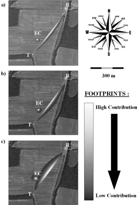
Fig. 1. Study area of Lamasqu`ere. Location of the Eddy
Covari-ance system (EC) with the scintillometer transmitter (T) and re-ceiver (R). Footprints are displayed for the three periods: (a) P1 (April), (b) P2 (June) and (c) P3 (September).
on a stable 3 m-high concrete tower built to avoid instrument oscillations due to strong wind. The path length between the transmitter and the receiver was approximately 567 m. The output signal, expressed as a voltage, was recorded by a low-power consumption computer at 1 kHz, and was filtered for absorption phenomena at 0.1 Hz (Meijninger et al., 2002b).Cn2 was calculated according to Eq. (2). A brief preliminary comparison of the CESBIO-built instrument to another LAS (METAIR group from Wageningen University and Research Center) was performed and provided a good correlation between the results of the two instruments.
During the intercomparison, the heights of both scintil-lometers were different,zLAS=6 m for the METAIR LAS and zLAS=3 m for the CESBIO LAS, but this height difference was accounted for in calculation of the sensible heat flux (H). Data from both scintillometers were found to be linearly re-lated:HLAS CESBIO=1.28∗HLAS METAIR(R2=0.981). The coefficient (1.28) was found to be consistent across a number of measurements, and was attributed to the greater
sensitiv-ity of the GRITE scintillometer to the focus of the detector and the effective diameter of the light beam (a misalignment of the instruments can reduce the effective diameter of the beam observed at the receiver). This phenomenon has been previously reported in other comparisons of multiple scin-tillometers, with relative differences ranged from 5% (Mei-jninger et al., 2002a) to 21% (Kleissl et al., 2008). Since our scintillometer was in the development stage when this work was conducted, a calibration campaign was conducted prior to each measurement period, to avoid flux overestimation due to misalignment. In addition, a threshold was imposed on the signal amplitude so as to avoid dew effects on scintillometer measurements. Hereafter, the fluxHestimated with the scin-tillometer will be referred to asHLAS.
An eddy covariance system was installed at mid-transect of the scintillometer light beam at a 3.65 m height. The EC system was equipped with a CSAT3 sonic anemometer (Campbell Scientific Ltd.) to measure wind speed fluctua-tions in three dimensions, as well as sonic temperature, and an IR gas analyzer Licor 7500 (Campbell Scientific Ltd.) was used to measure H2O and CO2 concentrations. Typi-cal meteorologiTypi-cal sensors were also added to the EC mast to provide mean values for atmospheric pressure, air tem-perature and relative humidity. The net radiation (RN)was
measured using a CNR1 (Campbell Scientific). Soil heat flux (G) was measured at a depth of 5 cm using three heat flux plates (hpf01, Hukseflux), and was corrected to consider the storage between the surface and the heat flux plate. All fluxes were averaged over 30-min periods, which provided a good trade-off between eddy sampling and the stationary as-sumption. Some corrections were applied to the EC system flux estimates, according to the recommendations of the Car-boEurope experimental program (Aubinet et al., 2000, 2003; Lee et al., 2004). Thus, wind speed measurements were cor-rected for double rotation, as advised for crop and grasslands sites. Corrections also accounted for the time lag between the sonic anemometer and the analyser data logger, and high fre-quency spectral losses, as well as humidity effects, addressed via the WPL correction (Webb et al., 1980).
As the scintillometer location is close to the forest, foot-print analyses have been performed using the model of Mei-jninger et al. (2002). The footprint analyses were conducted for the main wind directions during the selected periods and required values of LO, u∗, σv calculated with the Eddy
In order to ascertain whetherCT2 behaviour followed the MOST, observed values ofCT2(zLAS−d)2/3/T∗2were plot-ted against observed values of (zLAS−d)/LO on Fig. 2
for the entire dataset. The universal function proposed by Hill (1992) and de Bruin (1993) were also plotted on the figure, and fit well with previous results, although a slight underestimation was observed. Values ofT∗ andLO were
taken from the EC set-up (Hoedjes et al., 2007), while values ofCT2(zLAS−d)2/3/T∗2that diverged from Monin-Obukhov theoretical behaviour were rejected. Rejection criteria had a significant influence on results as they resulted in the exclu-sion of approximately 20% of the data.
3.1 Seasonal evolution of the Bowen ratio
Using Eq. (4), the Bowen ratio (β) is required to compute sensible heat flux from scintillometer measurements. In this study, β is estimated through the EC turbulent fluxesHEC andLvEEC. In order to improve the significance of the scin-tillometer measurements, which rely onβ, and to limit arte-facts due to EC measurements, severe criteria were used to eliminate non-relevantβ values. Specifically, large uncer-tainties in the Bowen ratio are known to arise from varia-tions in the turbulent fluxes measured by EC systems (mainly due to variations in latent heat fluxLvEEC). A threshold on flux values has been imposed to reject low flux : 7 W/m2for the sensible heat flux and 15 W/m2 for the latent heat flux (Billesbach et al., 2004). Data were also rejected from night time or thermally stable measurement periods, when LAS data might be affected by the accumulation of dew or water vapour.
Figure 3 shows mean dailyβvalues derived from EC data for the period from 1 January 2007 to 1 October 2007. Since the Bowen ratio is closely related to vegetation transpiration capacity, and therefore to vegetation phenology, Leaf Area Index (LAI: leaf surface area per unit of soil surface area), representing the relative surface area of transpiring leaves, was also plotted. Three specific sub-periods were identified over the study period that appeared to correspond to different vegetation life stages (see Fig. 3).
The first period studied was at the end of April (DoY 109 to 114), corresponding to the maximum measured LAI, which was approximately 3.5, and varied rapidly. The Bowen ratio was low for this period (β≈0.1), due to high transpiration rates from the vegetation (hveg=>0.6 m). The second period occurred in midJune (DoY 163 to 169), when vegetation became senescent; green LAI was close to 0 (as was the transpiration rate), but vegetation height reached its maximum (hveg=0.9 m) and the Bowen ratio reached the value β=1. The third period occurred at the beginning of September (DoY 248 to 254). Crops were harvested at this time, and the field was nearly completely covered by crop residue (resulting in low vegetation height: hveg≈0.15 m). Sensible heat flux predominated during this period, resulting in a high Bowen ratio (β≈2.8).
Fig. 2. Observed values ofCT2(zLAS-d)2/3 /T∗2plotted against
observed (zLAS−d)/LO during the 3 periods. Data that diverges
from MOST behavior are rejected. Solid line represents the scal-ing of the universal function given by Hill (1992) and dotted line represents the one by de Bruin (1993).
3.2 Comparison of the “classical” and “β-closure methods”
In this section, the two methods for computing the sensible heat flux are described. The various input and output param-eters of both methods are summarised in Table 1. All exper-imental input values are measured by the Eddy Covariance set-up, except for Cn2 (scintillometer) and various heights (d,z0,zEC,zLAS). Besides, output parameters are calculated by iterative procedures.
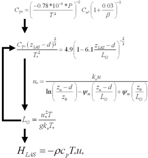
3.2.1 Classical method
Sensible heat flux (HLAS) computation using the classical it-erative method (WinLAS v.1 software) is described in Fig. 4. A first guess of the Obukhov length is required to initialise the calculation algorithm. The structure parameter of tem-perature (CT2) is first calculated from scintillometer signal and using the meteorological data and the Bowen ratio. This coefficient allows the calculation of the temperature scale of the Monin-Obukhov similarity theory (MOST) T∗ and the
friction velocityu∗ with this first value ofLO. This latter
term is then recalculated using the new values ofT∗andu∗.
When the algorithm forLOhas converged,T∗andu∗are
cal-culated again, andHLAScan then be deduced using Eq. (11). In the classical method, β is an input parameter esti-mated by independent measurements ofH andLvE (they
Fig. 3. Leaf Area Index (m2/m2) and mean daily values of the Bowen ratio according to the Day of Year (DoY) in 2007. The three periods are represented by grey boxes: P1 corresponds to Avril dataset (DOY 109 to 114), P2 to June one (DOY 163 to 169) and P3 to September one (DOY 248–254).
have been estimated using a 5-year dataset of EC measure-ments. The method used was reported by Hollinger and Richardson (2005), who developed a methodology using daily differenced measurements with equivalent environmen-tal conditions. Random errors in the flux calculated using our EC station data wereσLVE=0.134LvE+5.8,R2=86.5% and σH=0.117H+6.8,R2=76.4%. Finally, the random error law
for the Bowen ratio can be estimated for the same dataset, according to Gaussian error propagation:σβ=0.301β+0.02.
According to Fig. 4, the friction velocityu∗is calculated
iteratively using a profile approach (Eq. 8). However, u∗
could be estimated from turbulent data of the EC set-up. Asanuma et al. (2007) investigated the calculation of sensi-ble heat flux from sintillometer measurements on a homoge-neous to heterogehomoge-neous surfaces using values ofu∗provided
by the EC system, and concluded that the sensitivity ofHLAS tou∗ depends primarily on the stability index (z/LO) and
on the differences between the scintillometer and EC system footprints. As the error can be large, iterations onLOandu∗,
using the Eqs. (7) and (8), are rather advised for calculating HLAS. This point is further discussed with the experimental results.
3.2.2 “β-closure method”
In this method, we assume that the Bowen ratio has been cor-rectly measured, and that the energy budget can be balanced by redistributing the closure error across both fluxes (Foken, 2008). Using this assumption,βcan be expressed as (Bowen, 1926) :
β= HLAS
RN−G−S−HLAS
. (13)
Fig. 4. Schematic description of the classical method process.
Table 1. Input and output parameters that are required for the
clas-sical and “β-closure methods”.
Input parameters Output parameters
Classical method Cn2,T,u,P,z0,d,zLAS, H,LO,T∗,u∗ zEC,β
“β-closure method” (BCM) Cn2,T,u,P,z0,d,zLAS, H,LO,T∗,u∗,β zEC,G,RN
The iterative procedure described in the “classical method” is also applied, butCT2 is computed using the latter expres-sion forβ. However, becauseβ depends onHLAS, an extra iterative step is required (Fig. 5). The principle advantage of the “β-closure method” is that no turbulent flux measure-ments are necessary. Only the net radiation (RN) and the soil
heat flux (G) are required. In most cases, the impact ofS is also weak and can thus be neglected. Figure 5 describes the iterative procedure of the BCM. In this case, initial as-sumptions are needed for the Bowen ratioβand the Obukhov lengthLO. First,CT2 is calculated using a first guess forβ, andT∗andu∗are derived from a first guess forLO.
Subse-quently,LO is re-estimated andHLAS is computed usingT∗
andu∗, whereasβ is deduced from the energy balance
clo-sure (Eq. 13). When calculatedLOvalues converge,T∗and
u∗ are computed to estimate the final value of the sensible
balance closure, instead of being derived from the turbulent heat flux measurements (H andLvE). As the Bowen ratio
is determined iteratively, and not by measurement, its asso-ciated error (standard deviation) is null.
In order to evaluate the energy balance closure and its im-pact on the method, a parameter is introduced to characterise the percentage of closure. This parameter was calculated ac-cording to EC data, and was designated the energy balance fraction (or Energy Balance Ratio when averaged over a long period of time, Gu et al., 1999):
γ= H+LvE
RN−G−S
(14) This ratio can be represented by the available energy, which is the ratio of the difference between net radiation and the sum of soil heat flux and heat storage (RN−G−S), all
di-vided by the turbulent fluxes (H+LvE). For the three
pe-riods considered, the energy balance fraction was equal to 81%, which is quite typical for this type of surface (Fig. 6). 3.2.3 Uncertainty calculation
As measurement uncertainties (random and systematic er-rors) may affect the final estimation of the flux, it is worth comparing both methods in terms ofHLASuncertainty. Here, to determine the uncertainty ofHLAS, a standard deviation (σH) was calculated for both methods, according to formula
for Gaussian Error Propagation (Marx et al., 2008):
σH2=X
∂H
∂Inputi 2
σInput2i+
H
hi−Hdb
2 2
(15) whereσ is the standard deviation and Inputi corresponds to
the input variables of Table 1 (for the case of WinLas). The second term corresponds to the uncertainty in the univer-sal function, with Hhi and Hdb corresponding toHLAS
esti-mated with the different universal functions reported by Hill et al. (1992) and de Bruin et al. (1993), respectively. Marx et al. (2008) provides measurement uncertainties for the param-eters in Table 1:Cn2(0.5%),T (0.1 K),u(0.5%),P (100 Pa), z0 (10%),zLAS (0.5 m), zEC(0.1 m). The net radiation un-certainty was close to 5–6%, whereas the error in soil heat conduction measurements (G) was between 15% and 20% (Twine et al., 2000, Kohsiek et al. 2007). When attempting to determineHLAS uncertainty by the “β-closure method”, uncertainties onRN,GandS will be added to Eq. (15), as
they intervene in the energy balance closure.
Prior to investigating the influence of the Bowen ratio onHLAS estimation, a preliminary uncertainty analysis was performed. Assuming that the uncertainty on β is null, sensible heat flux values are calculated via the classical method, the uncertaintiesεin the flux estimates for each pe-riod (which correspond to the average value ofσH/HLAS over that period) are ε=11.3% in April (LAI maximum), ε=11.4% in June (senescence) and ε=12.1% in September
Fig. 5. Schematic description of the “β-closure method” algorithm.
Fig. 6. Turbulent heat fluxes (H+LvE) versus net radiation
mi-nus soil heat conduction and heat stockage (RN-G-S) for the
whole dataset. The best linear fit with a zero-origin is: H+Lv E=0.81(RN−G−S) with a correlation ofR2=0.79.
4 Results and discussion
For the three considered periods of 2007, the Bowen ratioβ varied between values of 0.02 to 4.86 (Fig. 3). Asβcan have very low values, it is important to quantify its influence both in terms of flux estimates and uncertainty. When a high de-gree of precision is required forHLAS flux values and little information is available regarding the Bowen ratio, the “β -closure method” (BCM) is quite attractive, as no direct mea-surements ofβare required. Indeed, it can be very useful for longterm experiments in which measurements ofβ are not accurate, due to a minimum instrumental set-up at the field site. To quantify the impact ofβon flux calculations, the ro-bustness of the classical and BCM methods was investigated during the year 2007.
4.1 Sensible heat flux calculated via the classical method
The Bowen ratio is first calculated with 30 min averaged val-ues ofHECandLvEEC. Then,HLASis estimated via the
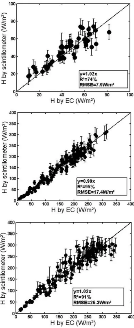
clas-sical method using theseβ values. Results are displayed for each period (April, June, September 2007) in Fig. 7, compar-ing scintillometer data versus the correspondcompar-ing EC fluxes.
It appears that both datasets are well correlated in June (HLAS=0.98HEC, R2=95%) and in Septem-ber (HLAS=1.02HEC, R2=91%). In April, when fluxes are weaker, the correlation remains satisfying (HLAS=1.02HECR2=74%).
Uncertainties related to the flux computation were also quantified. For the different periods, a 17.3% error inHLAS was obtained in April, 11.7% in June, and 12.1% in Septem-ber. The uncertainties in HLAS increased as the value of the Bowen ratio decreased. It must be noted that in our case, uncertainty inβ only considers random errors. If the valueσβ=0.18 given by Twine et al. (2000) is used, which
combines systematic and random errors, the predicted uncer-tainty inHLASis much higher (48% in April, 12.6% in June and 12.2% in September).
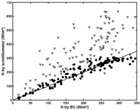
As we noticed formerly, the friction velocity can be either calculated iteratively or measured by the EC system. A com-parison has been performed using measurements of the fric-tion velocity (from the EC system) instead of iterative com-putation for the period P3 as both footprints (of the EC sta-tion and scintillometer) are superimposed in this period and βsensitivity ofHLASis negligeable. Then,HLASfluxes were calculated with the classical method considering a measured friction velocity. Results show large discrepancies while us-ingu∗from EC set-up, whereas u∗calculated by iterations
computesHLASwith greater accuracy (Fig. 8).
To sum up the results obtained with the classical method, it can be concluded that, for high Bowen ratio, the sensi-ble heat flux derived from scintillometerHLAS is well cor-related withHEC(R2>0.9). For low Bowen ratio, this cor-relation is weaker, due to the strongest sensitivity ofCT2 to
Fig. 7. Comparison between HECcalculated by Eddy Correlation,
andHLASderived from scintillometer, and calculated with the
Fig. 8. Comparison between HEC(Hby EC) and HLAS(Hby
scin-tillometer) calculated by the Classical method (black circles) or by the same method usingu∗calculated by EC set-up (grey triangles)
during the period P3. Black line stands for the 1:1 correlation.
the correction term inβ(Eq. 4) but remains acceptable. Be-sides, sensible heat fluxes derived from scintillometer mea-surements suffer from high meamea-surements uncertainties that range from 17% to 48% of the flux values. Moreover, as β=HEC/LvEEC, depends onHECand thatHLASis also com-pared toHEC, the independence of the results can be dis-cussed. Besides, EC set-up are often the only source of in-formation available for turbulent parameters asβ (Hartogen-sis et al., 2003; Kohsiek et al., 2006; Von Randow et al., 2008), which imposes to consider slight dependence ofHLAS toHEC.
4.2 Sensible heat flux values calculated via the “β -closure method” (BCM), balance fraction and Bowen ratio influence
The requirement ofβ values calculated every 30 min to min-imise measurement uncertainties could limit the use of scin-tillometry in wet conditions when the Bowen ratio is small. For instance, such conditions were encountered over the Amazonian forest by Da Rocha et al. (2003), who estimated a mean annual Bowen ratioβ of 0.17, or by Sadhuram et al. (2001), who found thatβ can be even smaller than 0.1 during monsoon periods or over open ocean waters. In our experimental site, 38% of the days in 2007 corresponded to a Bowen ratio smaller than 0.4. Using an alternative computa-tion method that does not include a measurement ofβcould thus extend the field of application of scintillometry. To this end, the accuracy and robustness of the “β-closure method” (BCM) were examined.
Hoedjes et al. (2002) applied this method to derive fluxes using scintillometry over an irrigated area in Mexico. Their measurements showed good correlations with EC results, and
Table 2. Correlation (R2) and linear fit between HLAS estimated
with the scintillometer according to both methods (the classical one and the BCM) and HECmeasured with ECstation.
Classical Method BCM γ β
April 1.02×(R2=74%) 0.95×(R2=57%) 78.5% 0.12 June 0.99×(R2=95%) 0.96×R2=94%) 79.7% 1.01 September 1.02×(R2=91%) 1.01×(R2=91%) 98.7% 2.8
displayed a tendency to overestimate the sensible heat flux in dry conditions. In the current study, the sensible heat flux was calculated similarly for the three selected periods. The influence of the two main parameters, the energy balance fraction (γ), and the Bowen ratio, was also analysed. The re-sults for the three periods are presented in Table 2. In April, βis very small (0.12) and the energy budget is poorly closed (γ=78.5%). In June, the energy balance fraction is still small (γ=79.7%) but the Bowen ratio increases (β≈1). In Septem-ber, the energy balance is almost closed (γ=98.7%), andβis high.
Performances of scintillometers to estimateH flux have already been studied in the case of homogeneous surface and showed high correlation withHEC(McAneney et al., 1995; De Bruin et al., 1995; Hoedjes et al., 2002). Then, the dis-cussion is focused on the comparison of both methods.
In a preliminary analysis, it can be observed that the “β -closure method” tended to give the same results as, classical method, especially during the June and September periods (Fig. 9). However,γ andβ seemed to affect the results of the “β-closure method” :HLASby BCM diverges fromHLAS by Classical method, when both parameters decreased. The influence ofβon this divergence is more stringent, as shown by the comparison of the April and June results (whereγ is approximately the same). It is evident that the decrease inβwas followed by an underestimation ofHLASby 6% in April, 3% in June and 1% in September. It can be noted that including the storage term (S) in the energy budget modified the finalHLAS estimates by less than 1%. Thus, this term can be neglected while using the “β-closure method” without significant error.
According to Gaussian Error Propagation calculations, and with assumed uncertainties of 6% forRN and 20% for (G+S), averaged uncertainties for the different periods were reduced to 18.4% in April, 12.8% in June, and 13.1% in September. The contribution of the error inRN and(G+S)
4.3 Moisture influence
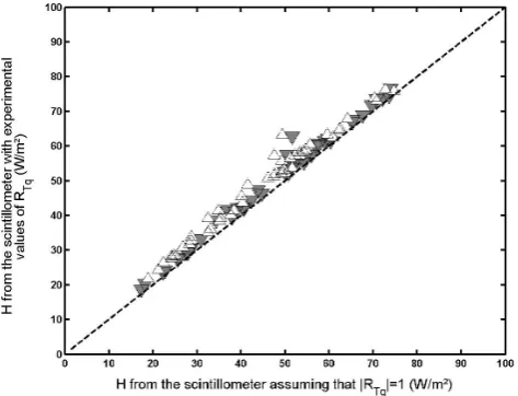
Further analysis has been performed to include the mois-ture effect (RT q) inHLAS computation with both methods. Moene (2003) estimated the possible error due to the ap-proximation of|RT Q|=1 in Eq. (4), to be up to 40% when
the Bowen ratio is low, and advised to neglect the correction term inβ. Furthermore, L¨udi et al. (2008) showed thatRT Q
is dependent upon the Bowen ratio. The lowest the Bowen ra-tio is, the worst the temperature and humidity are correlated. Then, according to this criteria the period P1 is the most sen-sitive period toRT Qfluctuations and needs to be further
in-vestigated to quantify the influence of the lack of correlation between temperature and humidity. Besides the influence of RT qis negligeable in June and September (Moene, 2003).
RT Qhas been calculated for the three periods, at the time
scale of 30 min. The averages values ofRT Qfor each period
is 0.76 for P1, 0.66 for P2, and 0.59 for P3, which are compa-rable with other authors. For instance, Sorbjan (1993) sums up the results of different experimentations and conclude that RT Qis between 0.6 and 0.8 in the surface boundary layer.
The sensible heat flux has been calculated with experimen-tal values ofRT Q, and was then compared to previous results
(where|RT Q|=1 is assumed) for the period P1 (Fig. 10). The
results show a relative underestimation ofHLASin April due to the approximation ofRT Q=1 of 6% (±3%) with the
Clas-sical method and 9% (±4%) with the BCM.
5 Conclusions
Measurements of the mass and energy exchanges between the surface and the atmosphere at the ecosystem scale are a major topic of many projects involved in land-surface mon-itoring (e.g., Sud Ouest project). Whereas Eddy Covariance (EC) stations provide local measurements, scintillometers are able to estimate the sensible heat flux from measurements of the structure parameter of refractive index,Cn2, integrated over distances up to several kilometres. However, their ac-curacy relies on the acac-curacy of the meteorological parame-ters required for calculating the sensible heat flux. Among these parameters, we focused on the Bowen ratio,β, which is the most sensitive to uncertainty in meteorological mea-surements, since it relies on the measurement of the turbu-lent fluxesH andLvE by standard EC systems. With the
objective of installing scintillometers as autonomous devices, there is a strong incentive to further investigate the depen-dence of the heat fluxes measured by these devices upon in-put values forβ. Therefore, two different computation meth-ods of the sensible heat flux were tested to evaluate the re-quirements for installing scintillometers in tandem with ad-ditional measurement devices in order to achieve a desired degree of accuracy.
Fig. 9. Comparison of the sensible heat fluxes derived from the
scintillometer HLAS with the “β-closure method” (BCM) versus
Fig. 10. Comparison betweenH calculated with the scintillome-ter considering a perfect temperature/humidity cross-correlation (RT Q=1), and with the measured one, for the period P1.
Clas-sical method is represented by grey triangles, and BCM by white triangles.
The influence of a measured Bowen ratio on flux calcula-tions was first studied via a “classical method” (WINLAS software) for three different periods of vegetation growth (April, June and September 2007). The sensible heat fluxH was calculated with 30 min-averaged values ofβ measured using an EC flux system. In June and September, whenβ>1, HLAS andHECare well correlated, and the uncertainty on HLAS measurement is around 12%. In April 2007, when the Bowen ratio was smallest (β=0.12), the correlation between HLASandHECdecreases (71%) due to the strongest sensitiv-ity ofHLASto the correction term inβ. Moreover, the lack of accuracy on β measurement for lowβ values produced an increase in the measurement uncertainty (between 17 and 48%).
The “β-closure method” is a useful alternative when infor-mation about the Bowen ratio is unavailable. In this case, the computational algorithm only requires net radiation and soil conductivity measurements to determine the Bowen ratio, as-suming that the energy balance is closed. With this method, the results are rather satisfying even in April, considering the small under-estimation of HLAS (<6%) even when the Bowen ratio was small. Furthermore, the uncertainty in HLAS was limited to 18.5% in April, and 13% in June and September. These findings suggest that at low Bowen ratios, fluxes can be estimated with accuracy and with less uncer-tainty using the BCM than with classical methods. In ad-dition, the BCM requires less instrumentation for turbulent measurements.
The approximation of a perfect correlation between tem-perature and humidity (RT Q=1) has been discussed in low
Bowen ratio conditions (April) which is the most sensitive case toRT Qfluctuations. RT Qvalues have been integrated
over 30 min and included into each computational method. It results in a relative underestimation ofHLAS, using|RT Q|=1,
between 6 and 9% in comparison withHLAS, using experi-mental values ofRT Q.
When using a scintillometer as an autonomous device, it is advisable to employ the “β-closure method”, as one can reduce the uncertainties in flux estimates caused by the lack of accuracy in the estimation ofβ, and by the systematic and random errors in measurements. An interesting perspective might be to test this calculation method under very wet con-ditions (such as measurement campaigns over lakes or open ocean), in which EC station installation is difficult.
Acknowledgements. The SudOuest experiment was supported by
the Conseil R´egional Midi-Pyr´en´ees, the CNES (Centre National d’Etudes Spatiales), and the Minist`ere de l’Environnement (GICC). It was also partly funded by the CarboEurope-IP program and CNRS/INSU. The authors would like to thank l’Ecole Sup´erieure d’Agriculture de Purpan and the congregation of Notre Dame de la Motte for welcoming us at the Lamasqu`ere site. We would like to express our gratitude to all of the technical teams (Herv´e Gibrin, Bernard Marciel). Finally, we are also very grateful to W. Koshiek for his helpful suggestions on the development of our scintillometer and to A. Moene for his help and comments regarding uncertainty calculations.
Edited by: G. Ehret
The publication of this article is financed by CNRS-INSU.
References
Andreas, E. L.: Estimating Cn2over Snow and Sea Ice from Mete-orological Data, J. Opt. Soc. Am., 5, 481–495, 1988.
Andreas, E.L.: Two-wavelength method of measuring path-averaged turbulent surface heat fluxes, J. Atmos. And Ocean Tech., 6, 280-292, 1989.
Asanuma, J. and Lemoto, K.: Measurements of regional sensible heat flux over Mongolian grassland using large aperture scintil-lometer, J. Hydrol., 333, 58–67, 2007.
Aubinet, M., Grelle, A., Ibrom, A., Rannik, ¨U., Moncrieff, J., Fo-ken, T., Kowalski, A. S., Martin, P. H., Berbigier, P., Bernhofer, C., Clement, R., Elbers, J., Granier, A., Gr¨unwald, T., Morgen-stern, K., Pilegaard, K., Rebmann, C., Snijders, W., Valentini, R., and Vesala, T.: Estimates of the annual net carbon and water exchange of forests: The EUROFLUX methodology, Adv. Ecol. Res., 30, 113–175, 2000.
Fluxes of carbon, water and energy of European forests. Eco-logical Studies, edited by: Valentini, R., 163, Springer, Berlin, Heidelberg, 9–35, 2003.
Bastiaanssen, W. G. M., Menenti, M., Feddes, R. A., and Holtslag, A. A. M.: A Remote Sensing Surface Energy Balance Algorithm for Land (SEBAL) – 1. Formulation, J. Hydrol., 212–213, 198– 212, 1998.
Billesbach, D. P., Fischer, M. L., Torn , M. S., and Berry, J. A.: A portable eddy covariance system for the measurement of Ecosystem-Atmosphere exchange of CO2, Water Vapor, and En-ergy, J. Atmos. Oceanic. Technol., 21, 684–695, 2004.
Bowen, I. S.: The ratio of heat losses by conduction and by evapo-ration from any water surface, Phys. Rev., 27, 779–787, 1926. Brotzge, J. A.: Closures of the surface energy budget, PhD Thesis,
The Univeristy of Oklahoma, March 2001, 208 pp., 2001. Businger, J. A., Miyake, M., Dyer, A. J., and Bradley, E. F.: On
the direct determination of heat flux near the ground, J. Appl. Meteor., 6, 1025–1031, 1967.
Dabberdt, W. F., Lenschow, D. H., Horst, T. W., Zimmerman, P. R., Oncley, S. P. and Delany, A. C.: Atmosphere-surface exchange measurements, Science, 260, 1472–1481, 1993.
Da Rocha, H.R., Goulden, M. L., Miller, S. D., Menton M. C., Pinto, L. D. V. O., de Freitas, H. C., and Silva Figueira, A. M.: Seasonality of water and heat fluxes over a tropical forest in eastern amazonia, Ecol. Appl., 14, No. sp4, 22–32, 2004. De Bruin, H. A. R, Kohsiek,W., van den Hurk, B. J. M.: A
veri-fication of some methods to determine the fluxes of momentum, sensible heat, and water vapor using standard deviation and struc-ture parameter of scalar meteorological quantities, Bound.-Lay. Meteorol., 63, 231–257, 1993.
De Bruin, H. A. R., Van den Hurk, B. J. J. M., and Kohsiek, W.: Ths Scintillation Method tested over a dry vineyard area, Bound.-Lay. Meteorol., 76, 25–40, 1995.
Dugas, W. A., Fritschen, L. J., Gay, L. W., Held, A. A., Matthias, A. D., Reicosky, D. C., Steduto, P. and Steiner, J. L.: Bowen ratio, eddy correlation, and portable chamber measurements of sensible and latent heat flux over irrigated spring wheat, Agric. For. Meteorol., 56, 1–20, 1991.
Foken, T.: The energy balance closure problem – An overview, Ecol. Appl., 18, 1351–1367, 2008.
Green, A. E. and Ayashi, Y.: Using the scintillometer over a rice paddy, Japan, J. Agric. Meteorol., 54, 225–231, 1998.
Gu, J., Smith, E. A., and Merritt, J. D.: Testing Energy Balance Closure with GOES retrieved Net Radiation and in Situ Mea-sured Eddy Correlation Fluxes in BOREAS, J. Geophys. Res., 104, 27–81, 1999.
Halldin, S. and Lindroth, A.: Errors in net radiometry: compari-son and evaluation of six radiometer designs, J. Atmos. Oceanic. Technol., 9, 762–783, 1992.
Hartogensis, O. K., Watts, C. J., Rodriguez, J.-C., de Bruin, H. A. R.: Derivation of the effective height for scintillometers: La Poza experiment in Northwest Mexico, J. Hydrol., 4, 915–928, 2003. Hill, R. J., Clifford, S. F. and Lawrence, R. S.: Refractive index
and absorption fluctuations in the infrared caused by tempera-ture, humidity and pressure fluctuations, J. Opt. Soc. Am., 70, 1192–1205, 1980.
Hill, R. J.: Implications of Monin-Obukhov Similarity Theory for Scalar Quantities, J. of Atm. Sci., 46, No.14, 1989.
Hill, R. J., Ochs, G. R., and Wilson, J. J.: Measuring Surface
Layer Fluxes of Heat and Momentum Using Optical Scintilla-tion, Boundary-Layer Meteorol., 58, 391–408, 1992.
Hoedjes, J. C. B., Zuurbier, R. M. and Watts, J. C.: Large aperture scintillometer used over a homogeneous irrigated area, partly af-fected by advection, Bound.-Lay. Meteorol., 105, 99–117, 2002. Hoedjes, J. C. B., Chehbouni, A., Ezzahar, J., Escadafal, R., and De Bruin, H. A. R.: Comparison of Large Aperture Scintillome-ter and Eddy Covariance Measurements: Can Thermal Infrared Data be Used to Capture Footprint Induced Differences?, J. Hy-drometeorol., 8 (2), 144–159, 2007.
Horst, T. W. and Weil, J. C.: How far is far enough? The fetch requirements for micrometeorological measurement of surface fluxes, J. Atm. Oc. Tech., 11, 1018–1025, 1994.
Kleissl, J., Gomez, J., Hong, S.-H., Hendrickx, J. M. H, Rahn, T., and Defoor, W. L.: Large Aperture Scintillometer Intercompari-son Study, Bound.-Lay. Meteorol., 128, 133–150, 2008. Kohsiek, W., Meijninger, W. M. L., deBrui, H. A. R., and Beyrich,
F.: Saturation of the large aperture scintillometer, Boundary-Lay. Meteorol., 121, 111–126, 2006.
Kohsiek, W., Liebethal, C., Foken, T., Vogt, R., Oncley, S. P., Bern-hofer, C., de Bruin, H. A. R.: The energy balance experiment EBEX-2000, Part III : Behaviour and quality of radiation mea-surements, Boundary-Lay. Meteorol., 123, 55–75, 2007. Konzelmann, T., Calanca, P., Muller, G., Menzel, L., and Lang, H.:
Energy balance and evapotranspiration in a high mountain area during summer, J. Appl. Meteorol., 36, 7, 966–973, 1997. Lamaud, E., Og´ee, J., Brunet, Y., and Berbigier, P.: Validation of
Eddy flux measurements above the Understorey of a Pine Forest, Agr. Forest. Meteorol., 106, 187–203, 2001.
Lee, X., Massman, W. J., and Law, B.: Handbook of Micromete-orology: A Guide for Surface Flux Measurement and Analysis, Kluwer, Dordrecht, The Netherlands, 250 pp., 2004.
Marx, A., Kunstmann, H., Schuttemeyer, D. and Moene, A. F.: Un-certainty analysis for satellite derived sensible heat fluxes and scintillometer measurements over Savannah environment and comparison to mesoscale meteorological simulation results, Agr. Forest. Meteorol., 148, 656–667, 2008.
McAneney, K. J., Green, A. E., and Astill, M. S.: Large-Aperture scintillometry: the homogeneous case, Agric. For. Meteorol., 76, 149–162, 1995.
Meijninger, W. M. L. and de Bruin, H. A. R.: The sensible heat fluxes over irrigated ares in western Turkey determined with a large aperture scintillometer, J. Hydrol., 229, 42–49, 2000. Meijninger, W. M. L., Hartogensis, O. K., Kohsiek, W., Hoedjes, J.
C. B., Zuurbier, R. M., and De Bruin, H. A. R.: Determination of Area-Averaged Sensible Heat Fluxes with a LargeAperture Scin-tillometer over a Heterogeneous Surface – Flevoland Field Ex-periment, Bound.-Lay. Meteorol., 105, 37–62, 2002a.
Meijninger, W. M. L., Green, A. E., Hartogensis, O. K., Kohsiek, W., Hoedjes, J. C. B., Zuurbier, R. M. and De Bruin, H. A. R.: Determination of area-averaged water vapour fluxes with large aperture and radio wave scintillometers over heterogeneous surface-Flevoland field experiment, Bound.-Lay. Meteorol., 105, 63–83, 2002b.
Society, 9.2, 2004.
Moene, A. F.: Effects of water vapour on the structure parameter of the refractive index for near-infrared radiation, Boundary-Layer Meteorol., 107, 635–653, 2003.
Nie, D., Kanemasu, E. T., Fritschen, L. J., Weaver, H. L., Smith, E. A., Verma, S. B., Field, R. T., Kustas, W. P., and Stewart, J. B.: An intercomparison of surface energy flux measurement systems used during FIFE 1987, J. Geophys. Res., 97, 18715– 18724, 1992.
Ochs, G. R. and Wilson, J. J.: A second-Generation Large-Aperture Scintillometer, NOAA Tech. Memo., ERL WPL-232, Env. Res. Lab, Boulder, CO, 24 pp., 1993.
Panofsky, H. A and Dutton, J. A.: Atmospherric Turbulence: Mod-els and Methods for Engineering Applications, J. Wiley, New York, USA, 397 pp., 1984.
Paulson, C. A. : The mathematical representation of wind speed and temperature profiles in the unstable atmospheric surface layer, J. Appl. Meteorol., 9, 857–861, 1970.
Sadhuram Y., Ramana Murthy, T. V., Sarma, Y. V. B., and Murthy, V. S. N.: Comments on On the estimation of overwater Bowen ratio from sea – air temperature difference., J. Phys. Oceanogr., 31, 1933–1934, 2001.
Sorbjan, Z.: Notes and Correspondaence : Monin-Obukhov Sim-ilarity for Refractive Index Revisited, J. Atmos. Sci., 50, 21, 3677–3679, 1993.
Twine, T. E., Kustas, W. P., Norman, J. M., Cook, D. R, Houser, P. R., Meyers, T. P., Prueger, J. H., Starks, P. J. and Wesely, M. L.: Correcting Eddy-Covariance Flux Underestimates over a Grass-land, Agr. Forest. Meteorol., 103, 279–300, 2000.
Von Randow, C., Kruijt, B., Holtslag, A. A. M., de Oliveira, M. B. L.: Exploring eddy-covariance and large-aperture scintillometer measurements in an Amazonian rain forest, Agr. Forest. Meteo-rol., 148, 680–690, 2008.
Wang, T., Ochs, G., and Clifford, S.: Saturation-Resistant optical scintillometer to measure Cn2, J. Opt. Soc. Am., 68, 334–338, 1978.
Webb, E. K. Pearman, G. I., and Leuning, R.: Correction of flux measurements for density effects due to heat and water vapor transfer, Q. J. Roy. Meteor. Soc., 106, 85–100, 1980.
Wesely, M. L.: The combined effect of Temperature and humidity Fluctuations on Refractive index, J. Appl. Meteorol., 15, 43–49, 1976.