R E S E A R C H
Open Access
The difficulty of protein structure alignment
under the RMSD
Shuai Cheng Li
Abstract
Background: Protein structure alignment is often modeled as thelargest common point set(LCP) problem based on the Root Mean Square Deviation (RMSD), a measure commonly used to evaluate structural similarity. In the problem, each residue is represented by the coordinate of the Cαatom, and a structure is modeled as a sequence of 3D points. Out of two such sequences, one is to find two equal-sized subsequences of the maximum length, and a bijection between the points of the subsequences which gives an RMSD within a given threshold. The problem is considered to be difficult in terms of time complexity, but the reasons for its difficulty is not well-understood. Improving this time complexity is considered important in protein structure prediction and structural comparison, where the task of comparing very numerous structures is commonly encountered.
Results: To study why the LCP problem is difficult, we define a natural variant of the problem, called theminimum aligned distance(MAD). In the MAD problem, the length of the subsequences to obtain is specified in the input; and instead of fulfilling a threshold, the RMSD between the points of the two subsequences is to be minimized. Our results show that the difficulty of the two problems does not lie solely in the combinatorial complexity of finding the optimal subsequences, or in the task of superimposing the structures. By placing a limit on the distance between consecutive points, and assuming that the points are specified as integral values, we show that both problems are equally difficult, in the sense that they are reducible to each other. In this case, both problems can be exactly solved in polynomial time, although the time complexity remains high.
Conclusions: We showed insights and techniques which we hope will lead to practical algorithms for the LCP problem for protein structures. The study identified two important factors in the problem’s complexity: (1) The lack of a limit in the distance between the consecutive points of a structure; (2) The arbitrariness of the precision allowed in the input values. Both issues are of little practical concern for the purpose of protein structure alignment. When these factors are removed, the LCP problem is as hard as that of minimizing the RMSD (MAD problem), and can be solved exactly in polynomial time.
Keywords: Protein Structure, Alignment, RMSD, LCP
Background
A common approach to understand the properties of a protein is to compare it to other proteins. Proteins that are similar, in terms of either their amino acid sequences or 3-dimensional structures, often share similar functions, or are related evolutionarily. The latter, structural compari-son, is particularly interesting since protein structures are
Correspondence: [email protected]
Department of Computer Science, City University of Hong Kong, Kowloon, Hong Kong
known to be more evolutionarily conserved than the bio-logical sequences which encode them. Furthermore, pro-teins of similar structures may have similar functionality, even when their sequences differ [1].
Structural comparison is typically a problem of align-ing two sets of 3-dimensional coordinates. (In most of the known structural alignment problems, each point is the 3D coordinates of the Cα atom, one per residue. Hence, a structure can be modeled for structural alignment pur-pose as a sequence of 3D points.) The alignment usually involves a rigid transformation to superimpose the two sequences of points, and a mapping which specifies the
matched points. The parameters to optimize in the align-ment may differ in different situations, because it is not easy to single out a set of parameters that best captures the similarity between two given structures [2]. In many situations, the alignment needs not match between every point in the two sequences. At present, there is a consen-sus among molecular biologists in the use of the following two parameters [2-4]:
1. the number of residues (points) or percentage of total residues (points) matched in the alignment.
2. the root mean square deviation (RMSD) of the matched residues (points).
In general, the RMSD need not be minimized. It suf-fices that it is within a reasonable threshold. Hence, a good alignment is customarily taken to be one which max-imizes the number of residue matches, within a given RMSD threshold. Many structural alignment methods are based on this principle. The computational complexity of finding an optimal solution to the problem is not well understood. Shibuya et al. formulated a restricted ver-sion of the problem, and showed the problem to NP-hard when the dimensionality is arbitrary. It is open whether their problem is NP-hard in 3-dimension [5]. Other prob-lems related to structural comparison based on the RMSD have been found to be difficult. For example, the prob-lem of finding a substructure from multiple 3-dimensional structures which minimizes the total RMSD, is NP-hard [6].
For the variants of the alignment problem that are not based on the RMSD, we have the following results. When the objective is to maximize the number of point matches which are no more than a threshold distance apart, the problem is solvable inO(n32.5)time, wherenis the num-ber of points [7]. Thecontact map overlapproblem, where a graph is created out of each structure, and the prob-lem is one of comparing the two graphs, is NP-hard [8], and remains NP-hard even when we require points that are matchable to be within a threshold distance [9]. These results, together with an early result which shows a related problem called threading to be NP-hard [10], have traditionally led molecular biologists to believe that the structural alignment problem is difficult in general (e.g. [11-13]), even though a PTAS exists for the problem under a broad class of distance measures [14]. Heuristic algorithms have also been proposed for many variants of structural alignment problem [15-23]. While these meth-ods perform reasonably well in general, they provide no guarantee on the quality of their results.
As noted by Shibuya et al., relatively few theoretical results have been obtained on problems defined over the RMSD, and the general problem of structural alignment under the RMSD remains open [5]. At present, whether
the problem is intractable or not is not only of theoretical interests but also of practical concerns, due to advances in protein structure prediction which requires the compar-ison of very numerous structures. In this paper we show mathematical insights and techniques which we hope will lead to practical algorithms for the problem.
We first show that the difficulty of the problem does not lie solely in the individual components of their require-ment. More precisely,
– if either a mapping that contains the optimal mapping is known (Theorem 3), or
– if the optimal superposition is known (Lemma 1),
then the problem can be solved in polynomial time. Our study shows that the difficulty of the LCP problem is also very much due to the two factors: (1) the problem allows the input coordinates to be of any arbitrary preci-sion, and (2) it assumes no limit on the distance between two consecutive Cαatoms.
We consider the case where the input coordinates are integral, and the distance between two consecutive points is restricted. The first requirement is practical since in protein structures, coordinates are typically specified to a fixed precision (e.g. three decimal places in protein struc-tures [24]), and can be trivially scaled up to integral values. Similar assumptions are made in Euclidean problems such as the Euclidean TSP [25]. The second requirement like-wise does not add any restriction to the problem of protein structure alignment, since there is a natural upper bound (∼3.8 ˚A) to the distance between two Cα atoms. In this case, the following results hold.
– Given a polynomial time algorithm for finding a largest alignment of RMSD below a thresholdd, one can efficiently compute an alignment of a given size which minimizes the RMSD (Theorem 7). (Since the other direction is easy, this shows that the two problems are of similar difficulty.)
– The structural alignment problem under the RMSD is solvable exactly in polynomial time (Theorem 10).
Preliminary
Notations and definitions
Problem statements
We now state our problems. The main problem we con-sider is the largest common point set (LCP) problem under the RMSD, a well-known problem in protein struc-ture alignment. In the LCP, the objective is to find a mapping of the largest cardinality where the RMSD of the matched points is no more than a given threshold (Table 1).
We do not require the optimal superposition ofPand
Qin the output, since that can be computed fromP,Q, andf in linear time [26]. We refer tof as analignment. An alignment can besequentialornon-sequential: an align-ment issequential iff for any two points pi1, pi2 ∈ P,
where the correspondingf(pi1) = qj1 andf(pi2) = qj2,
we havei1 < i2 iffj1 < j2. Otherwise the alignment is
non-sequential. The LCP problem which requires align-ments to be sequential is said to besequential, otherwise it isnon-sequential. We mainly discuss sequential align-ment in this paper. The techniques developed can be easily adapted to the non-sequential case. Given two equal-sized sequencesP =(p1,. . .,pn)andQ, together with a bijec-tionf betweenPandQ, the root mean square deviation (RMSD) is defined as
RMSD(P,Q)=min t
1≤i≤n||t(f(pi))−pi||2
n , (1)
wheretis a rigid transformation. The RMSD, with its cor-responding transformation t, can be computed in linear time [26].
A natural variant of the LCP problem is to minimize the RMSD instead of maximizing the size of the mapping, as follows. Given an integer, find subsequences of size of the input, such that the RMSD between the points of the subsequences is minimized. We call this problem the minimum aligned distance (MAD) problem (Table 2).
Clearly, if the MAD problem is solvable in polynomial time, then the LCP problem is solvable in polynomial time. However, the other direction is unclear. Theorem 7 will show that forP andQof integral coordinates, if the LCP problem is solvable in polynomial time, then the MAD problem is solvable in polynomial time.
Table 1 Largest Common Point (LCP) set problem definition under RMSD
LCP problem by the RMSD measure
Input: sequencesP=(p1,. . .,pn),Q=(q1,. . .,qm)and distance
thresholdθ∈R. Without loss of generality assumem≥n.
Output: (i) subsequencesP⊆P,Q⊆Q,|P| = |Q|, and
(ii) bijectionf:P→Q, fulfilling the following conditions:
(A)RMSD(P,f(P))≤θ,
(B) the scorel= |P|is maximized.
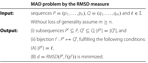
Table 2 Minimum Aligned Distance (MAD) problem definition under RMSD
MAD problem by the RMSD measure
Input: sequencesP=(p1,. . .,pn),Q=(q1,. . .,qm)and∈I.
Without loss of generality assumem≥n.
Output: (i) subsequencesP⊆P,Q⊆Q,|P| = |Q|, and
(ii) bijectionf:P→Q, fulfilling the following conditions:
(A)|P| =,
(B)d=RMSD(P,f(p))is minimized.
We letPˆ,Qˆ,ˆf,anddoptdenote an optimalP,Q,f,l andd, respectively. The optimal rigid transformation for superimposingPˆ andQˆ is denotedT, and can be com-puted from Pˆ, Qˆ and ˆf. The symbol cmaxP denotes the largest value in the coordinates ofP,cmaxQ the largest value in the coordinates ofQ, andcmax=max{cmaxP ,cmaxQ }, and we know thatcmax=O(n)for protein structures.
Results for general LCP and MAD
Complexity of the LCP and MAD when the optimal superposition is known
Since two point sequences with a known mapping can be superimposed optimally under the RMSD in linear time [26], it is natural to ask if the difficulty in LCP or MAD lies solely in the combinatorial complexity of finding the opti-mal subsets, i.e.PˆandQˆ. Our results show the contrary: if the optimal superpositionT is known, both problems can be solved in polynomial time.
We first consider the sequential case. Letdp,q= ||t(p)− q||2and let M[i,j;k] denote the minimum squared sum cost ofkpair matches for the point sets(p1,p2, ...,pi)and (q1,q2, ...,qj). If 1≤k≤ , 2≤i≤mand 2≤j≤ n, we have a recurrence relation of
M[i,j;k]=max
⎧ ⎨ ⎩
M[i−1,j−1;k−1]+dpi,qj, M[i,j−1;k] ,
M[i−1,j;k]
⎫ ⎬ ⎭
(2)
The base case of the recursion is obvious. Dynamic programming can be employed to fill up the respective
M[i,j;k] values. After all the values are filled, one can find the maximumk, such that the squared sum is no more thankθ2for the LCP problem. The MAD problem can be solved similarly.
The non-sequential case can be similarly solved using the maximum-flow minimum-cost problem [27]. The fol-lowing lemma states these results.
Complexity of the LCP and MAD when the matching between the point sets is known
We next ask if the difficulty in the LCP and MAD could be due to the task of superimposingPandQin an opti-mal manner to identify the subsetsPˆ andQˆ. To examine this possibility, we remove the combinatorial task of exam-ining each of the possible mapping between the points, by assuming a bijection F which contains the optimal mapping. (Note that this results in the problem known asmodel superpositionin structural biology.) Again, our results show the resultant LCP and MAD problems to be solvable exactly in polynomial time.
Assume that F is a bijection that maps points in P to points inQ. LetP = (p1,. . .,pl)be the domain ofFand
Q=(q1,. . .,ql)be the range ofF. Without loss of gener-ality assume thatFis sequential, and henceF(pi)=qi.
One can exhaustively evaluate all the subsequences of
Pfor one with the least RMSD. However, since the num-ber of such subsequences is exponential inl, this does not immediately give us a polynomial time solution.
If a rigid transformation T for Q is given, and all the pairs (pi,qi), 1 ≤ i ≤ l are sorted according to the value ||T(pi) − qi||, the MAD problem is then to choose the first pairs from (pi,qi), 1 ≤ i ≤ l, and the LCP problem is to choose the first pairs, such that RMSD((p1, ...,p),(q1, ...,q)) ≤ θ and = l or
RMSD((p1, ...,p,p+1),(q1, ...,q,q+1)) > θ. This gives us an incentive to obtain a total ordering of||T(pi)−qi||, which will allow us to solve the MAD problem by selecting the firstpairs in the ordering. The set of transformations which produce the same total according to||T(pi)−qi||, yield the same result for the MAD problem, and therefore these transformations are equivalent. This enables us to design a discrete version of the problem.
For clarity, we first present an algorithm with only trans-lation.
With translations only
Consider two pairs (pi,qi) and (pj,qj). The transforma-tionsT to separate the two types of transformations that
||T1(qi) − pi|| > ||T1(pj) −qj|| and ||T2(qi) −pi|| <
||T2(pj)−qj||are the transformations where
||T(qi)−pi||2− ||T(pj)−qj||2=0. (3)
Let • denote dot product. If the transformation is a translationt, we have
||T(qi)−pi||2− ||T(qj)−pj||2 = ||qi−pi−t||2− ||qj−pj−t||2
=
v=x,y,z (vq
i−vpi−vt)
2−
v=x,y,z (vq
j−vpj −vt)
2
= ||qi−pi||2− ||qj−pj||2
−2t•((qi−pi)−(qj−pj))=0 (4)
Consider the space of all translation vectors inR3, and consider each vector as a point in this space (not the space that P andQ are in). The values that the variable t in Equation 4 may take form a plane in this translation space. The plane partitions the translation space into two types of translations, T1 and T2 say, where||T1(qi) − pi|| >
||T1(pj)−qj||and||T2(qi)−pi|| < ||T2(pj)−qj||. Since there arelpairs, there areO(l)planes, which partition the space intoO(l3)cells.
The translations in each cell result in the same ordering of the pairs with respect to||T(pi)−qi||. For each cell, this total order can be obtained inO(l)time from any given total order of its neighbor cells, since the change isO(1). Therefore, the MAD solution can be obtained in amor-tized timeO(l)for each cell, and the LCP solutions thus can be obtained in timeO(l2). Hence the total runtime is ofO(4)for the MAD problem, andO(5)for the LCP problem of translations, with the given mappingF.
With rigid transformations
The rigid transformations which separate the two rela-tions||T1(qi)−pi||>||T1(pj)−qj||and||T2(qi)−pi||<
||T2(pj)−qj||are as in Equation 3.
Suppose the rigid transformations T is composed of a rotationRand a translationt.
||T(qi)−pi||2− ||T(qj)−pj||2 = ||R(qi)−pi−t||2− ||R(qj)−pj−t||2 = ||R(qi)−pi||2− ||R(qj)−pj||2
−2t•[(R(qi)−pi)−(R(qj)−pj)] (5)
A rotation matrix contains three variables, which is specified using three angles, sayα1,α2,α3, each from−π to π. Let ri = cosαi, si = cosαi, then Equation 5 can be considered as a polynomial of nine variables in degree six. The nine variables areri,siand the three variables for translation. In total, there areO(l)such polynomials.
We know the following theorem from the literature.
Theorem 2. [7,28] Given a set of k polynomials,P = {f1, ...,fk}, where each polynomial has a maximum degree of s, contains at most r variables, and in addition all the coefficients are rational, then all the sign conditions can be determined by O(k(k/r)rsO(r))arithmetic operations. A sign condition V is the vector of signs for some point u ∈ Rk; that is, V = (sign(f
1(u)), ...,sign(fk(u))). Two points u,u∈Rkare equivalent if their sign condition vectors are the same.
Theorem 3.Given a bijection F:P→Q, where|P| = l, then the MAD problem can be solved in O(l10)time and
the LCP problem can be solved in O(l11)time.
Results assuming integral coordinates and restricting distance between points
One possible contributing factor to the difficulty of the LCP problem could be its flexibility in allowing input coordinates of any arbitrary precision. This is because intuitively, this arbitrariness in the precision introduces the burden of examining the solution space in an unbounded manner. However, such an exhaustive search is not necessary for the purpose of protein struc-ture comparison, since coordinates of protein strucstruc-tures are specified only to three decimal places in the commonly used PDB format.
In this section, we restrict the precision in which the input coordinates may be specified. Without loss of gen-erality, we assume that the input coordinates are given in integers, since numbers of any fixed precision can be triv-ially scaled up to integral values. This assumption is used to obtain Lemma 5 and Theorem 7.
We also place an upper bound on the distance between consecutive points according to the structure of proteins. As a result,cmaxis bounded byn, as follows.
Points drawn from protein structures have upper bounds on their diameters because they are connected, and many are globular.
- For a connected structure, the points are at most O(n)distance apart. That is,cmaxis ofO(n). - For a globular structure, the points are at most
O(n1/3)distance apart [14]. That is,cmaxis of O(n1/3).
Given a pointp, let thexcoordinate ofpbe denotedxp. Similarly, we can defineypandzp. Without loss of gener-ality, we assume that the first point of a protein structure is at the origin. The largest coordinate of a protein is bounded byO(n), and the largest coordinate of a globular protein structure is bounded byO(n1/3); that is
max
p∈P,v=x,y,z|vp| =O(n), if P is a protein structure (6)
max
p∈P,v=x,y,z|vp|=O(n
1/3), if P is a globular protein structure
(7)
Our results show that, under these two conditions, 1. the LCP problem is of similar difficulty as the MAD
problem, and
2. both problems can be solved exactly in polynomial time.
Properties of protein structures
Upper and lower bounds of RMSD
We first establish some bounds to the RMSD. The mini-mum RMSD is zero ifT bringsQˆ to coincide exactly with
ˆ
P. This case is referred to as the exact matching, which can be easily solved by the method in [29]. However, if we assume the RMSD to be non-zero, then a lower bound and an upper bound for it can be computed.
Let π be a permutation of {1, ...,}. For the sequence
X=(x1,. . .,xn), letdXi,j, 1≤i,j≤n, denote the Euclidean distance betweenxi andxj. The following results, which are proven in the Appendix, can be obtained.
Lemma 4.
1
√
2
/2
i=1 |d
ˆ P
π(i),π(i+/2)−d
ˆ Q
π(i),π(i+/2)|2
RMSD(Pˆ,Qˆ).
Lemma 5 (Lower bound).If RMSD(Pˆ,Qˆ) = 0, then RMSD(Pˆ,Qˆ)≥
√
12c2 max−
√
12c2 max−1 √
2 .
Lemma 6(Upper bound).RMSD(Pˆ,Qˆ)≤4√3cmax.
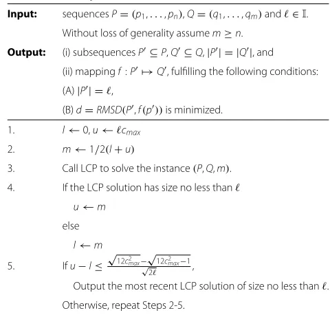
Using an algorithm for the LCP to solve the MAD problem Suppose there is a polynomial time algorithm for solving the LCP problem. To use it to solve the MAD prob-lem, we assume thatdopt ∈[l,u], for some reallandu, l ≤ u. We use a binary search strategy in the interval [l,u], as shown in Table 3, to search for the minimum
Table 3 Employing an algorithm for the LCP problem to solve the MAD problem
Input: sequencesP=(p1,. . .,pn),Q=(q1,. . .,qm)and∈I.
Without loss of generality assumem≥n.
Output: (i) subsequencesP⊆P,Q⊆Q,|P| = |Q|, and
(ii) mappingf:P→Q, fulfilling the following conditions:
(A)|P| =,
(B)d=RMSD(P,f(p))is minimized.
1. l←0,u←cmax
2. m←1/2(l+u)
3. Call LCP to solve the instance(P,Q,m).
4. If the LCP solution has size no less than
u←m
else
l←m
5. Ifu−l≤ √
12c2
max− √
12c2
max−1
√
2 ,
Output the most recent LCP solution of size no less than.
value such that the LCP solution size is . However, the search will not terminate if an arbitrary accuracy of the
dopt value is required. We prove below that the accuracy ofdopt can be defined by polynomially many bits. Given two threshold t1 andt2, assume that we obtain two dif-ferent LCP solutions, and the RMSD values of the two solutions areθ1andθ2, whereθ1> θ2. Similar to the argu-ments in Lemma 5, the difference between θ1 andθ2is at least
√
12c2 max−
√
12c2 max−1 √
2 . Therefore if two consecutive binary search operators have the difference of the thresh-old values below
√
12c2 max−
√
12c2 max−1 √
2 , the search can be terminated. The values oflanduare the same as in the previous subsection. Hence,
Theorem 7.Solving the MAD problem is equivalent to solving O(logcmax)instances of the LCP problem.
Since the reduction from the LCP problem to the MAD problem is obvious, we conclude that the two problems are of similar difficulty.
Polynomial time algorithm
We now show that under the two conditions, the LCP and MAD problem can be solved in polynomial time.
As shown in the ‘Complexity of the lCP and mAD when the optimal superposition is known’ section, when the optimal superposition is known, there are polynomial time algorithms for LCP and MAD. We consider an enu-meration of all the possible superpositions. Under the two conditions, we claim that there are at most polynomially many such superpositions.
First, if we knowPˆ andQˆ, then optimal superposition can be computed in the following two steps:
1. TranslatePˆandQˆ such that their centroids are at the origin.
2. Then, rotateQˆ to find the superposition with the minimum distance [26].
Denote the translations to obtain the optimal solution for P and Q astP andtQ, respectively, and denote the optimal rotation byRˆ.
We now show that one needs to examine only poly-nomially many translations and rotation combinations to discover the values fortP,tQ, andRˆ. These numbers can be effectively bounded by nwhen properties of protein structures are taken into account. We first describe these properties.
Number of translations
The centroid of Pˆ is
p∈Pˆp
. To bring Pˆ to origin, the translation is−
p∈Pˆp
. Clearly, all the three coordinates of−p∈Pˆpare integers since all the coordinates of the
points inp ∈ Pare integers. The value of x-coordinate of −
p∈Pˆp
is bounded by −
p∈Pˆxp
≤
p∈Pˆc
max P
≤
cmax. Similarly, all the three coordinates of the translation
−
p∈Pˆp
are bounded within the interval [−cmax,cmax]. To obtain an optimal MAD solution, the translation onPˆ must be in the form of I, whereIis an integer. Since it is possible to examine all the possible values forI, we have the following result.
Lemma 8. tP,tQ∈ {I/| −cmax≤I≤cmax}3.
Number of rotations
With the centroids ofPˆandQˆ translated to the origin, we proceed to identify the rotation in our algorithm. LetXP denote the vectorxp1, ...,xpfor structureP. Similarly we
defineYPandZP.
LetPˆt=(p1−t, ...,p−t)andQˆt=(q1−t, ...,q−t),
pi∈Pˆ,qi∈Qˆ.
GivenPˆandQˆ, to compute the rotationRˆ, the first step is to create the 3×3 matrix, which is (from [26])
M=
⎛ ⎜ ⎜ ⎝
XPˆtP •XQˆtQ XPˆtP •YQˆtQ XPˆtP •ZQˆtQ
YPˆ
tP •XQˆtQ YPˆtP•YQˆtQ YPˆtP•ZQˆtQ ZPˆtP •XQˆtQ ZPˆtP •YQˆtQ ZPˆtP •ZQˆtQ
⎞ ⎟ ⎟
⎠ (8)
Each above matrix is decomposed by the singular value decomposition, and a rotation matrix is produced here-after.
We know that the coordinate of each point in the protein is within the interval [−cmax,cmax]. This implies that for U=X,Y,ZandV=X,Y,Z,
UPˆtP •VQˆtQ =
k=1
(pi,k−tP)(qj,k−tQ)≤
k=1
(2cmax)2
≤4c2max.
Also, it is clear thatUPˆ
tP •VQˆtQ is in the form ofI/
2, whereI is an integer. The matrix in Equation 8 has nine elements; we denotee ∈ Mifeis one of these elements. The following lemma follows.
Lemma 9. For each element e ∈ M in Equation 8, e ∈ {I/2| −43c2
max≤I≤43c2max}.
Polynomial time algorithm
To compute the optimal MAD solution, we first enumer-ate all the possible translations and rotations. A solution is computed for each translation and rotation combination according to Lemma 1. An optimal solution can be chosen from these computed solutions (Table 4).
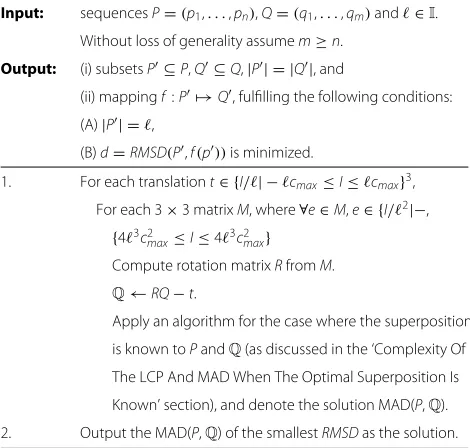
Table 4 A polynomial time algorithm for the MAD problem
Input: sequencesP=(p1,. . .,pn),Q=(q1,. . .,qm)and∈I.
Without loss of generality assumem≥n.
Output: (i) subsetsP⊆P,Q⊆Q,|P| = |Q|, and
(ii) mappingf:P→Q, fulfilling the following conditions:
(A)|P| =,
(B)d=RMSD(P,f(p))is minimized.
1. For each translationt∈ {I/| −cmax≤I≤cmax}3,
For each 3×3 matrixM, where∀e∈M,e∈ {I/2|−, {43c2
max≤I≤43c2max}
Compute rotation matrixRfromM. Q←RQ−t.
Apply an algorithm for the case where the superposition
is known toPandQ(as discussed in the ‘Complexity Of
The LCP And MAD When The Optimal Superposition Is
Known’ section), and denote the solution MAD(P,Q).
2. Output the MAD(P,Q) of the smallestRMSDas the solution.
optimal rotation matrix, it suffices that we try all the pos-sible values for each entry in Equation 8. Since there are 27c18
maxmatrices, the number of total transformations to examine is bounded byO(33c34
max). It takes timeO(mn) to identify the MAD solution for each transformation. An LCP solution can be obtained by iterating from 1 to min{m,n}for the MAD problem.
The running time consists of the productions of three parts: the number of possible translations, the number of possible rotation matrix, and the running time for given a rotation matrix and a translation combination (that is, the running time when then transformation is known). These numbers are bounded bycmax, which is bounded by mwhen we consider the properties of protein structures. Likewise,cmaxis polynomial with respect to the input size if coded in unary.
Theorem 10.The MAD problem can be solved in O(34m25n)time for protein structures, and in O(34m9n)
time for globular protein structures. The LCP problem can be solved in O(35m25n)time for protein structures, and in O(35m9n) time for globular protein structures. Both the MAD and LCP problems are pseudo-polynomially solvable for general point sets.
Conclusions
We studied the LCP problem under the RMSD in this paper. As it turns out, the difficulty of the problem does not lie in its combinatoric aspect or its structural superpo-sition aspect alone. That is, if the problem is hard, then it must be a consequence of both aspects. Our results show that if one is allowed to compromise on one of the aspects, then the problem is solvable exactly in polynomial time.
Regrettably, we do not see how the optimal solution can be obtained in both cases.
On the other hand, we showed an encouraging result: There is a polynomial time algorithm which solves the problem optimally, if one restricts the input coordinates in the problem to be integral, and places a limit on the dis-tance between consecutive points. These requirements do not pose any restriction to typical uses in the analysis of protein structures, since protein structures are specified only to a fixed precision in practice, and there is an upper bound to the distance between protein residues.
One problem is that our proposed polynomial time algorithm remains high in time complexity. We hope that the present work will provide the foundation for future efforts to obtain algorithms with lower runtime complexities.
Appendix
In this Appendix, we include the proofs of the results in the paper which have been omitted to enhance readability.
Lemma 4.
1
√
2
/2
i=1 |d ˆ P
π(i),π(i+/2)−d ˆ Q
π(i),π(i+/2)|2
≤RMSD(Pˆ,Qˆ).
Proof.Without loss of generality, we just show that 1
√ 2
/2
i=1 |d ˆ P
i,i+/2−d ˆ Q
i,i+/2|2≤RMSD(Pˆ,Qˆ). Let
ri= ||T(qi)−pi||2+ ||T(qi+/2)−pi+/2||2,
ui= pi,pi+/2, and
vi= qi,qi+/2, where 1≤i≤ /2.
First, we prove thatri ≥ |ui−vi|2/2, for 1≤i≤ /2. We first superimposeui andvi to optimize the squared sum; that is, to find transformationT such that||T(qi)− pi||2+ ||T(qi+/2)−pi+/2||2is minimized. The cen-troids have to coincide to minimize the squared distance. Assume the centroids are at the origin and that the angle between−−−→(o,pi)and(−−−→o,qi)isα, whereois the origin, then by trigonometry
||T(qi)−pi||2+ ||T(qi+/2)−pi+/2||2
=2[(1/2× ||ui||)2+(1/2× ||vi||)2
−2×1/2||ui||×1/2||vi|| ×cosα]
≥ (||ui|| − ||vi||)2 2
ri≥
(||ui|| − ||vi||)2 2
Putting things together, we have
RMSD(Pˆ,Qˆ) ≥
r1+. . .+r/2
≥
(u1−v1)2+. . .+(u/2−v/2)2 2
≥ √1
2
/2
i=1
|diPˆ,i+/2−diQˆ,i+/2|2
Lemma 5.If RMSD(Pˆ,Qˆ) = 0, then RMSD(Pˆ,Qˆ) ≥
√
12c2 max−
√
12c2 max−1 √
2 .
Proof. If RMSD(Pˆ,Qˆ)is non-zero, then there is at least a pair of indices i and j, such that ||dPˆ
i,j − d ˆ Q
i,j|| > 0. According to Lemma 4,
RMSD(Pˆ,Qˆ)≥ √1 2
|dPiˆ,j−diQˆ,j|2= |d ˆ P i,j−d
ˆ Q i,j|
√
2 >=
12c2 max−
12c2 max−1
√
2 .
Lemma 6. RMSD(Pˆ,Qˆ)≤4√3cmax.
Proof. Denote the furthest point to the origin inP as
pmax, and the furthest point to the origin inQasqmax. Then,
×RMSD2(Pˆ,Qˆ)
=
i=1
||T(qi)−pi||2
≤
i=1
(||qi−pi||)2
≤
i=1
max{||qmax−pmax||2,||qmax+pmax||2}
≤max{||qmax−pmax||2,||qmax+pmax||2}
≤(2(cmax+cmax)2+(cmax+cmax)2+(cmax+cmax)2)2
=48c2max
Abbreviations
LCP: Largest Common Point set; RMSD: Root Mean Square Deviation; MAD: Minimum Aligned Distance.
Competing interests
The authors declare that they have no competing interests.
Authors’ contributions
SCL conceived of the results herein and wrote the manuscript.
Acknowledgements
This work is supported by the CityU SRG 7002731. The author thanks the useful discussions with Prof. Richard M. Karp
Received: 8 December 2011 Accepted: 17 December 2012 Published: 4 January 2013
References
1. Perutz MF, Rossmann MG, Cullis AF, Muirhead H, Will G:North ACT: Structure of myoglobin: a three-dimensional Fourier synthesis at 5.5 Angstrom resolution.Nature1960,185:416–422.
2. R Kolodny PK, Levitt M:Comprehensive evaluation of protein structure alignment methods: scoring by geometric measures.J Comput Biol2005,346(4):1173–1188.
3. Sippl MJ:On distance and similarity in fold space.Bioinformatics2008, 24(6):872–873.
4. V A Ilyin CML A Abyzov:Structural alignment of proteins by a novel TOPOFIT method, as a superimposition of common volumes at a topomax point.Protein Sci2004,13(7):1865–1874.
5. Shibuya T, Jansso J, Sadakane K:Linear-time protein 3-D structure searching with insertions and deletions.Algorithms Mol Biol2010, 5(7):1–8.
6. Bu D, Li M, Li SC, Qian J, Xu J:Finding compact structural motifs.Theor Comput Sci2009,410:2834–2839.
7. Amb ¨uhl C, Chakraborty S, G¨artner B:Computing Largest Common Point Sets under Approximate Congruence.InESA ’00: Proceedings of the 8th Annual European Symposium on Algorithms, Volume 1876 of Lecture Notes in Computer Science. Saarbr ¨ucken, Germany: Springer-Verlag ; 2000:52–63. 8. Goldman D, Papadimitriou CH, Istrail S:Algorithmic Aspects of Protein
Structure Similarity. New York City, NY, USA: IEEE Computer Society; 1999. 9. Li SC, Ng YK:On protein structure alignment under distance
constraint.In20th International Symposium on Algorithms and Computation, ISAAC 2009, Proceeedings, Volume 5878 of Lecture Notes in Computer Science. Honolulu, HI, USA: Springer; 2009:65–76.
10. Lathrop RH:The Protein Threading Problem With Sequence Amino Acid Interaction Preferences Is NP-Complete.Protein Eng1995, 7:1059–1068.
11. Godzik A:The structural alignment between two proteins: is there a unique answer?Protein Sci1996,5(7):1325–1338.
12. Eidhammer I, Jonassen I, Taylor WR:Structure Comparison and Structure Patterns.J Comput Biol2000,7(5):685–716. 13. Zhao Z, Fu B, Alanis FJ, Summa CM:Feedback algorithm and
web-server for protein structure alignment.J Comput Biol2008, 15(5):505–524.
14. Kolodny R, Linial N:Approximate Protein Structural Alignment in Polynomial Time.Proc Natl Acad Sci2004,101:12201–12206. 15. Akutsu T, Tashimo H:Protein structure comparison using
representation by line segment sequences.InProc. Pacific Symposium on Biocomputing ’96. Hawaii, USA: World Scientific Press; 1996:25–40. 16. Alexandrov NN:SARFing the PDB.Protein Eng1996,9(9):727–732. 17. Caprara A, Lancia G:Structural alignment of large-size proteins via
lagrangian relaxation.InRECOMB ’02: Proceedings of The Sixth Annual International Conference on Computational Biology. New York, NY, USA: ACM; 2002:100–108.
18. Comin M, Guerra C, Zanotti G:PROuST: A Comparison Method of Three-Dimensional Structure of Proteins using Indexing Techniques.J Comp Biol2004,11:1061–1072.
20. Gibrat JF, Madej T, Bryant SH:Surprising similarities in structure comparison.Curr Opin Struct Biol1996,6(3):377–385.
21. Holm L, Sander C:Protein structure comparison by alignment of distance matrices.J Mol Biol1993,233:123–138. [http://dx.doi.org/10. 1006/jmbi.1993.1489].
22. Lancia G, Carr R, Walenz B, Istrail S:101 optimal PDB structure alignments: a branch-and-cut algorithm for the maximum contact map overlap problem.InRECOMB ’01: Proceedings of The Fifth Annual International Conference on Computational Biology. New York, NY, USA: ACM; 2001:193–202.
23. Singh AP, Brutlag DL:Hierarchical Protein Structure Superposition Using Both Secondary Structure and Atomic Representations.In Proceedings of the 5th International Conference on Intelligent Systems for Molecular Biology. Halkidiki, Greece: AAAI Press; 1997:284–293. 24. Berman HM, Westbrook J, Feng Z, Gilliland G, Bhat TN, Weissig H,
Shindyalov IN, Bourne PE:The protein data bank.Nucl Acids Res2000, 28:235–242.
[http://nar.oxfordjournals.org/cgi/content/abstract/28/1/235]. 25. Papadimitriou C:The Euclidean Traveling Salesman Problem is
NP-Complete.Theoretial Compututer Sci1977,4(3):237–244.
26. Arun KS, Huang TS, Blostein SD:Least-squares fitting of two 3-D point sets.IEEE Trans Pattern Anal Mach Intell1987,9(5):698–700.
27. Ahuja RK, Magnanti TL, Orlin JB:Network Flows: Theory, Algorithms, and Applications. Englewood Cliffs, NJ: Prentice Hall; 1993.
28. Basu S, Pollack R, Roy MF:A New Algorithm to Find a Point in Every Cell Defined by a Family of Polynomials(Caviness B, Johnson J, eds.) Springer Vienna: Springer-Verlag; 1998.
29. de Rezende PJ, Lee DT:Point Set Pattern Matching in d-Dimensions.
Algorithmica1995,13(4):387–404.
doi:10.1186/1748-7188-8-1
Cite this article as:Li:The difficulty of protein structure alignment under the RMSD.Algorithms for Molecular Biology20138:1.
Submit your next manuscript to BioMed Central and take full advantage of:
• Convenient online submission
• Thorough peer review
• No space constraints or color figure charges
• Immediate publication on acceptance
• Inclusion in PubMed, CAS, Scopus and Google Scholar • Research which is freely available for redistribution