R E V I E W A R T I C L E
Open Access
Algorithmic approaches to protein-protein
interaction site prediction
Tristan T Aumentado-Armstrong
1,2†, Bogdan Istrate
1,2†and Robert A Murgita
3*Abstract
Interaction sites on protein surfaces mediate virtually all biological activities, and their identification holds promise for disease treatment and drug design. Novel algorithmic approaches for the prediction of these sites have been produced at a rapid rate, and the field has seen significant advancement over the past decade. However, the most current methods have not yet been reviewed in a systematic and comprehensive fashion. Herein, we describe the intricacies of the biological theory, datasets, and features required for modern protein-protein interaction site (PPIS) prediction, and present an integrative analysis of the state-of-the-art algorithms and their performance. First, the major sources of data used by predictors are reviewed, including training sets, evaluation sets, and methods for their procurement. Then, the features employed and their importance in the biological characterization of PPISs are explored. This is followed by a discussion of the methodologies adopted in contemporary prediction programs, as well as their relative performance on the datasets most recently used for evaluation. In addition, the potential utility that PPIS identification holds for rational drug design, hotspot prediction, and computational molecular docking is described. Finally, an analysis of the most promising areas for future development of the field is presented.
Keywords: Prediction algorithm, Protein-protein interaction, Protein-protein interface, Protein-protein binding, Feature selection, Protein structure, Interface types, Machine learning, Biological databases, Homology
Background
Interactions between proteins drive the majority of cellular mechanisms, including signal transduction, metabolism, and senescence, among others. The identifi-cation of the surface residues mediating these processes, known as protein-protein interaction sites (PPISs), holds great therapeutic potential for the rational design of molecules modulating or mimicking their effects. Fur-ther, knowledge of the interacting sites can aid in other domains of computational biology, including PPI net-work construction and simulated docking. However, biochemical identification methods, such as experimental alanine scanning mutagenesis and crystallographic com-plex determination, are costly and time-consuming [1,2]. Such methods also consider only sites of the complex under examination, disregarding disparate sites involved
*Correspondence: [email protected] †Equal Contributors
3Department of Microbiology and Immunology, McGill University, Montreal, Canada
Full list of author information is available at the end of the article
in other interactions [3,4]. In response to these shortcom-ings, computational methods for the prediction of PPISs have been developed, starting with Jones and Thornton’s pioneering analysis of surface patches [5,6], and many predictors have since been published [7-43], utilizing a wide variety of algorithmic approaches to the problem.
This review will first provide a systematic analysis of the features and datasets used in PPIS prediction, from both a theoretical and application-oriented standpoint. An examination of the algorithms used in a selected set of the most recent PPIS predictors is also given, show-casing the diversity of the latest methods employed in this endeavour, as well as the potential for combining or extending them. This is complemented by a compar-ative evaluation of the performance of these predictors. Because it most accurately simulates the missing infor-mation inherent in real-world applications, we focus on the general case of PPIS prediction: using only a sin-gle unbound protein structure, without knowledge of an interacting partner, to predict the binding site of that pro-tein at the amino acid scale. Finally, the applications of
PPIS prediction and promising areas for future improve-ments are also discussed.
Interaction types
Virtually all cellular machinery is composed of pro-teins, whose functions are mediated through biomolecu-lar interactions; these serve to transmit signals and traf-fic molecular materials throughout the cell, as well as to form larger multimeric complexes capable of more complex behaviour [44,45]. These interactions occur pre-dominantly at conserved interfaces on the surfaces of the folded protein structures, often resulting in allosteric changes in the flexible conformations of the partners that alter their functions [46]. The potential biomedi-cal utility of interface identification makes the prediction of PPISs a critical endeavour, which necessitates theo-retical knowledge of the various types of protein-protein interaction sites.
One major distinction is between obligate complexes, which, by definition, do not form their
characteris-tic structure in vivo unless bound, and non-obligate
complexes, which can exist as stable monomers [47,48]; complexes are also divided along a continuum between transient and permanent interactions [49], based on temporal length or energetic strength [48,50-52]. Many methods are designed to predict transient interfaces (TIs) [8,17,22,28,35-37,53,54], as they have greater phar-macological relevance, particularly for signal trans-duction cascades [50,52]. However, TIs tend to be more difficult to predict than permanent interfaces [18,20,23,27,33,39,52,55], possibly resulting from the weaker nature of the interaction manifesting itself as a weaker signal in the properties defining the interacting residues [27,33,52]. However, the existence of fewer train-ing examples due to data gathertrain-ing difficulties may also play a role [47,49,56-58]. In general, TIs are less evolu-tionarily conserved than permanent interfaces [50,59-61], but more conserved than the rest of the protein sur-face [48]. Further, TIs tend to be more compact [51] and richer in water (i.e. more prone to water-mediated bind-ing) [51,62,63]. They also differ in residue propensities [18], including fewer hydrophobic [64] and more polar residues [65]. Thus, unsurprisingly, training on one inter-face type to predict on the other tends to decrease scores [18,33], though this is sometimes not the case [13]. Gen-erally, analysis of transient versus permanent complexes uses predefined sets [13,60,66] or programs designed to separate them [52,67-69].
All interfaces have distinctive “core” and “rim” regions, with core regions exhibiting lower sequence entropy (higher conservation) than rim [70], as well as reduced tolerance for water and decreased polarity [71-73]. The core of interfaces may be more readily predictable than the rim [7,33], likely for the same reason (i.e. stronger
characterizing signal) that permanent PPISs are easier to predict than TIs.
Upon binding, many proteins undergo conformational changes [51,74], which some interface predictors take into account [4,37,38,75]. Large-scale conformational change, such as a disorder-to-order shift [76], is believed to make prediction more difficult for computational protein-protein docking [77,78]; some PPIS predictors also have this difficulty [7,16,25,28,34,35], though several do not [12,32,42].
Datasets
Sources of training data
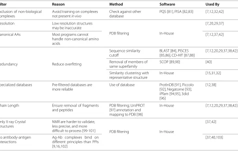
The majority of predictors based on machine learning (ML) rely on sets of structural information to train their learners, mainly curated from the PDB [79]. However, in the process of mining this database, it is necessary to filter out molecules that are not of sufficient quality or utility for use in the training set [37,80]. An overview of these filters is presented in Table 1.
Performance benchmark datasets
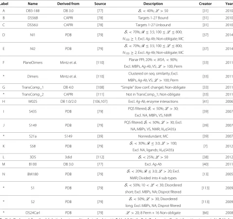
Due to the wide range of techniques used by existing predictors, an objective performance evaluation requires the use of standardized datasets that encompass as much of the diversity of proteins and interfaces as possible [75,104,105]. This includes sets such as the Docking Benchmark set, created in 2003 [106] and updated 3 times since its inception [77,107,108], which has seen signifi-cant use among PPIS predictors in its original, unedited form [12,18,28,103,109], as well as in modified forms [12,42,42,109]. All widely used modern testing sets are presented in Table 2.
Features
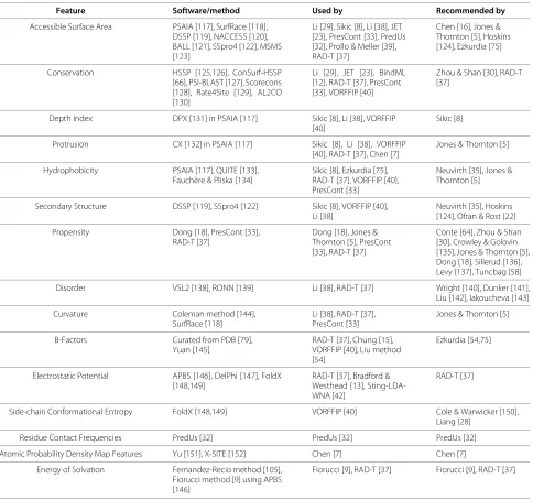
Characterizing features have been used to predict PPISs since the founding of the field [5], and have since been combined with ML algorithms of increasing sophistica-tion. While no single feature appears to possess suffi-cient information to allow prediction on its own, certain attributes have been consistently favoured, such as conser-vation and hydrophobicity. Recently, the use of databases of precalculated features, instead of on-the-fly calcula-tions, has gained popularity, via databases such as AAIn-dex [114,115] and Sting [116]. The most popular features, as well as references detailing their utility and procure-ment, are presented in Table 3.
Evolutionary metrics Conservation scores
Table 1 Filters used to curate protedatasets for use in training PPIS predictors, including the reasoning behind their use, the methods and specific software used to implement them, as well as references detailing the predictors making use thereof
Filter Reason Method Software Used By
Exclusion of non-biological complexes
Avoid training on complexes not presentin vivo
Check against other database
PQS [81], PISA [82,83] [7,12,32,42]
Resolution Low resolution structures may be inaccurate
PDB filtering In-House
[7,20,29,37]
Canonical AAs Most programs cannot handle non-canonical amino acids
[7,12,37,42]
Redundancy Reduce overfitting
Sequence similarity cutoff
BLAST [84], PISCES [85,86], CD-HIT [87,88]
[7,12,20,29,37,38,42]
Removal of members of same superfamily
SCOP [89,90] [40]
Similarity clustering with representative structure
In-House [15,31,32]
Specialized databases Pre-filtered databases are more reliable
Use of database ProtInDB [91], Piccolo [92], Negatome [93], iPfam [94,95], 3did [96]
[12,38]
Chain Length Ensure removal of fragments and peptides
PDB filtering; UniPROT [97] annotation and mapping to PDB [98]
In-House [7,12,20,29,37,38,42]
Only X-ray Crystal Structures
NMR are harder to validate, less precise, and more
difficult to process [99-101] PDB filtering In-House
[37,42]
No antibody-antigen interactions
Ag-Ab complexes bind on different principles than PPIs [9,16,102]
[37,40,103]
claiming that interface residues are not highly differ-entially conserved compared to the rest of the protein [156,157] or that evolutionary measures alone are of lim-ited predictive accuracy [22,39,158,159]. Some PPIS pre-dictors do not use conservation [7,8] or note that its use makes little difference [27,39]. On the other hand, a num-ber of analytical studies have found greater conservation among interface residues [16,30,55,160] and that conser-vation holds predictive utility [40,161]. Such conflicting conclusions may be a result of the different datasets and methods used to compute conservation.
Regardless, numerous PPIS predictors have made heavy use of residue conservation features [13,16,21,22,33, 35-38,40,41,162], including several based almost solely on evolutionary metrics [12,20,23,52,163], suggesting such measures do indeed have significant predictive power. In terms of generality, evolutionary methods can be more widely applicable than physicochemical ones, as the latter characteristics may differ markedly between functional sites, whereas conservation patterns in the former may be more easily recognizable [164]. Further, sequence conservation-based predictors do not require structural information [14,22,36]. However, since evolu-tionary methods are non-specific enough to be used for
identification of any type of functional site [165-169], this lack of specialization may reduce performance for PPIS prediction specifically [4]. Unsurprisingly, conser-vation is not helpful for interfaces selected by non-evolutionary means, such as antigen-antibody complexes [16,102] (which require separate specialized predictors [170]).
Predictors employ a number of methods to extract evo-lutionary features. Commonly, a multiple sequence align-ment (MSA) from BLAST [84] or PSI-BLAST [127] is used to derive conservation scores, in conjunction with substitution matrices (e.g. Dayhoff [171], BLOSUM [172], or position-specific) [13,14,33,38,41], often in combina-tion with informacombina-tion theoretic measures (generally based on Shannon entropy [173]) [18,27,33,39]. Some predic-tors [14,37,40] use previously developed programs for computing conservation [128-130,174-176].
Sequence homology
Table 2 Datasets Used to Evaluate Predictors in Table 4, including the source from which they were derived, as well as the publication in which they were created using the requirements in the “Description” column
Label Name Derived from Source Description Creator Year
A DB3-188 DB 3.0 [77] Si<40%;L >50 [31] 2010
B DS56B CAPRI [78] Targets 1-27 Bound [31] 2010
C DS56U CAPRI [78] Targets 1-27 Unbound [31] 2010
D NI1 PDB [79] Si<70%;R≤3.5; 100≤L ≤800; [37] 2014
N100≥1; Excl.Ag-Ab; Non-obligate; MC
E NI2 PDB [79] Si<70%;R≤3.5; 100≤L ≤800; [37] 2014
N100≥2; Excl.Ag-Ab; Non-obligate; MC
F PlaneDimers Mintz et al. [110] Planar PPI; 20%<MSAi<90%; [33] 2011 Excl. MBPs,Ag-Ab, VS;L >100; Perm
* Dimers Mintz et al. [110] Clustered on seq. similarity; Excl. [33] 2011
MBPs,Ag-Ab, VS;L >100; Perm
G TransComp_1 DB 4.0 [108] “Simple” (low conf. change); Non-obligate [33] 2011
* TransComp_2 CAPRI [111] Not in TransComp_1; Non-obligate [33] 2011
H W025 DB 1.0/2.0 [106,107] Excl.Ag-Ab, enzyme interactions [41] 2006
I S435 PDB [79] PQS filtered;Si<50%;L >30; [39] 2007
Excl. NA, MBPs, VS, NMR
J S149 PDB [79] PQS filtered;Si<50%;L >30; Excl. [39] 2007
NA, MBPs, VS, NMR;NH(S435)
* S21a S149 [39] Nonredundant; MC [39] 2007
K S58 PDB [79] Si<30%;R≤3.0;L >100; [7] 2012
Excl. NA, ligands;NH(S435)
L 3DS 3did [112] Si<25%;L >50 [38] 2012
M B100 DB 3.0 [77] Excl.Ag-Ab [40] 2011
N BM180 PDB [79] Si<20%;R≤3.0;L >20; Excl. [13] 2005
NMR; Divided into 4 sub-types
* S1 PDB [79] Si<50%; 10<L <30; Disordered [113] 2009
short; Excl. MBPs, NA; Disprot filtered
* S2 PDB [79] Si<50%;L >30; Disordered [113] 2009
long; Excl. MBPs, NA; Disprot filtered
* DS24Carl PDB [79] L >20; 8 Perm + 16 Non-obligate [66] 2008
The “Label” column defines the alphabetic character used to refer to the dataset in Table 4. “∗” in the “Label” column signifies that the set is not presented in Table 4 as it is not widely used.Siis the sequence identity redundancy cutoff,Lis the amino acid length of the chain,Ris the resolution cutoff in angstroms,N100≥nrequires
that the number of interface residues per 100 residues in a given protein to be greater thann,Ag-Abrefers to antigen-antibody complexes,MSAiis the sequence identity redundancy cutoff for chains in an MSA, VS refers to Viral Subunits, NA refers to Nucleic Acids,NH(x)refers to a set being non-homologous to setx, MC
denotes that both the monomer and the complex to which it belongs are known.
constructing phylogenetic distance trees to extract a residue ranking based on evolutionary importance, then using this to derive likely PPISs. Similarly, BindML [12] uses local MSAs, specialized substitution matrices, and phylogenetic tree construction to obtain the likelihood that a given patch MSA belongs to a PPIS (described below). HomPPI [20] derives linear combinations of BLAST statistics correlated to conservation score in
known interfaces, allowing an estimation of conservation in unknown interfaces.
Structural homology
Table 3 Compilation of selected software/methods used to compute features described in Features section, including the predictors utilizing each and the publications describing their utility and recommending their use
Feature Software/method Used by Recommended by
Accessible Surface Area PSAIA [117], SurfRace [118], DSSP [119], NACCESS [120], BALL [121], SSpro4 [122], MSMS [123]
Li [29], Sikic [8], Li [38], JET [23], PresCont [33], PredUs [32], Prollo & Meller [39], RAD-T [37]
Chen [16], Jones & Thornton [5], Hoskins [124], Ezkurdia [75]
Conservation HSSP [125,126], ConSurf-HSSP [66], PSI-BLAST [127], Scorecons [128], Rate4Site [129], AL2CO [130]
Li [29], JET [23], BindML [12], RAD-T [37], PresCont [33], VORFFIP [40]
Zhou & Shan [30], RAD-T [37]
Depth Index DPX [131] in PSAIA [117] Sikic [8], Li [38], VORFFIP [40]
Sikic [8]
Protrusion CX [132] in PSAIA [117] Sikic [8], Li [38], VORFFIP [40], RAD-T [37], Chen [7]
Jones & Thornton [5]
Hydrophobicity PSAIA [117], QUITE [133], Fauchère & Pliska [134]
Sikic [8], Ezkurdia [75], RAD-T [37], VORFFIP [40], PresCont [33]
Neuvirth [35], Jones & Thornton [5]
Secondary Structure DSSP [119], SSpro4 [122] Sikic [8], VORFFIP [40], Li [38]
Neuvirth [35], Hoskins [124], Ofran & Rost [22]
Propensity Dong [18], PresCont [33], RAD-T [37]
Dong [18], Jones & Thornton [5], PresCont [33], RAD-T [37]
Conte [64], Zhou & Shan [30], Crowley & Golovin [135], Jones & Thornton [5], Dong [18], Sillerud [136], Levy [137], Tuncbag [58]
Disorder VSL2 [138], RONN [139] Li [38], RAD-T [37] Wright [140], Dunker [141], Liu [142], Iakoucheva [143]
Curvature Coleman method [144], SurfRace [118]
Li [38], RAD-T [37], PresCont [33]
Jones & Thornton [5]
B-Factors Curated from PDB [79], Yuan [145]
RAD-T [37], Chung [15], VORFFIP [40], Liu method [54]
Ezkurdia [54,75]
Electrostatic Potential APBS [146], DelPhi [147], FoldX [148,149]
RAD-T [37], Bradford & Westhead [13], Sting-LDA-WNA [42]
RAD-T [37]
Side-chain Conformational Entropy FoldX [148,149] VORFFIP [40] Cole & Warwicker [150], Liang [28]
Residue Contact Frequencies PredUs [32] PredUs [32] PredUs [32]
Atomic Probability Density Map Features Yu [151], X-SITE [152] Chen [7] Chen [7]
Energy of Solvation Fernandez-Recio method [105], Fiorucci method [9] using APBS [146]
Fiorucci [9], RAD-T [37] Fiorucci [9], RAD-T [37]
and even general functional sites [183]. Importantly, struc-ture evolves more slowly than sequence and may have more powerful signals for conservation [184,185]. Predic-tors using structural homology have verified this proposi-tion [15,21,31,32,66,162,186].
The main issue with the use of structural homologs, or with predictors requiring structural information in gen-eral, is the paucity of usable structures [15,47,105,187], particularly when considering the relatively small size of the PDB (∼80,000 structures, including redundancy)
compared to the number of sequences known (∼17
million non-redundant sequences) [36,188], though this can be partly circumvented by using local (rather than
Physicochemical characteristics
Physicochemical properties have long been used for inter-face prediction [102]. The observed trend of increased hydrophobicity in interfaces compared to non-interacting surface patches [5,195-197], as well as the proposed pat-tern of a highly hydrophobic central region surrounded by polar residues [71,198], has been used with success in sev-eral recent predictors [8,33,37,40,75]. Additionally, elec-trostatic potential [13,42] and energy of desolvation [9] have shown utility as discriminative properties of PPISs [13,37,42]. B-factors (Debye-Waller temperature factors) [15,40] and disorder measures [37,38] in prediction soft-ware are also useful, with interface sites shown to be more disordered [38,140,141] yet also appearing to have lower B-factors than other surface patches [15,28,35,54,150]. Further, the decreased flexibility implied by decreasing B-factors is confirmed by the observation that interface residues minimize the entropic cost of complex forma-tion [28] by avoiding the sampling of alternative side-chain rotamers [40,150].
Statistical measures Propensity
Residue propensity, which measures PPIS amino acid composition, has been used in the characterization of interface types (e.g. homodimers versus heterodimers [16,199], permanent versus transient [18,80], biologi-cal versus non-biologibiologi-cal [200]) or subtypes (e.g. core versus rim [72,201]), in hotspot prediction [160,202], and evolution [203], as well as in PPIS prediction [13,28,33,35,37,41,204,205]. In general, polar amino acids are statistically disfavoured in interfaces sites, with the exception of arginine [18,35]. Further, while propen-sity differences are relatively minor between complex types, greater favouring of cysteine and leucine has been observed in permanent (but not transient) interfaces [18]. In general, predictors [13,35,37] use a variant of the fol-lowing equation to compute propensity based on amino acid frequencies:
prop(r)= countint(r)/|Interface| countsur(r)/|Surface|
where countint(r) and countsur(r) are the frequencies of occurrence of residuerin interfaces and on protein sur-faces, respectively, and |Interface| and |Surface| denote the sizes of these sets. More sophisticated extensions include using combinations of residues [33] (combinato-rially expanding the number of possiblervalues, though amino acid categories can reduce this [206]), weighting by accessibility [28,205], or computing binary profiles [18].
Atomic contact probability density maps
The packing preferences and geometries of atomic pro-tein structures have long been studied as a characterizing
feature of association [207], via probability density maps (PDMs) describing likelihoods of contacts [7,151,152]. Advantageously, PDMs can be derived from the intra-molecular contacts in the protein interior and are hence less limited by the structural information available [7,152]. While contacts in the protein interior differ from those in interfaces (e.g. artefactual interactions from structural constraints [152] or greater contribution of electrostatics to folding than binding [208]), these differences appear to be relatively minor [196,209-211], particularly when the interface core is mainly considered [137].
Recently, 3D PDMs were used as input features for PPIS prediction [7]. By projecting onto a previously described coordinate system [152], interacting contacts can then be added to the density map, allowing preservation of both magnitude and direction. Based on a similar method applied to protein folding [212], “co-incidental" interac-tions (due to proximal atoms forced together by structure constraints) [7,151] were filtered out.
These density maps can then serve as PPIS prediction features: given query protein P, feature vector vi = < ai1,. . .,ain > ∀i ∈ P, whereaij represents the
distance-weighted normalized sum of PDM values of atomiwith
interacting atom typej, andnis the number of interact-ing atom types (31, based on current works [7,151]). The resulting attribute vector setV = {vi∀i∈P}is amenable to ML-based PPIS prediction.
Structural geometry
Solvent accessible surface area
Often chosen as one of the most discriminatory features by a wide array of predictors [8,23,29,31-33,37-39], the Solvent Accessible Surface Area (SASA) of residues is thought to be of significant importance in PPIS prediction. Jones and Thornton [5,6] were among the first to suggest that high solvent accessibility is indicative of a residue’s participation in an interaction site. The relationship was further validated by Chen and Zhou on a set of 1256 non-homologous protein chains [16], as well as by Hoskins et al. [124], who also accounted for the relative con-tributions of both the main and side chains (polar and non-polar) of the protein.
3-D characteristics
PPISs have long been thought to posses distinct 3-dimensional characteristics that allow them to be dis-tinguished from the rest of the protein surface [5]. In particular, curvature has been singled out as an important 3D structural characteristic [33,37,38,186], with interface sites thought to be significantly more concave than the rest of the protein surface, lending stability and specificity to the interface [38].
complementarity, in which one of the proteins in a com-plex contains a concave binding site, while the interaction site on its partner exhibits convexity, in order to bind “snugly” [213]. Interestingly, Nooren and Thornton [48] showed that transient PPISs not only tend to be more planar than their permanent counterparts, but that there is a gradient even within transient sites, with “stronger” sites exhibiting greater curvature than those in “weaker” transient interactions.
Similarly, secondary structural characteristics have been used in several predictors [8,22,38,102], but have also elicited dispute regarding their utility and biological inter-pretation. Specifically, some studies [35,124] have found that β-sheets are favoured in interface sites while α -helices are more prevalent over the rest of the protein surface, though others disagree [38,102].
Depth and protrusion indices
As discussed previously, interfaces are rich in hydropho-bic residues, which is superficially incongruous with the finding that interfaces tend to have a higher solvent accessibility than non-interface patches. This has been explained by Li et al. [38], who, along with Sikic et al. [8] and Segura et al. [40], found the depth and protrusion features to be the most highly discriminatory features of their respective predictors. Thus, interface residues tend to have a higher average depth index (are more deeply buried), while maintaining a higher side-chain protrusion (leading to the observed increase in solvent accessible surface area) [38].
Algorithmic approaches
While there exist previous reviews on PPIS predic-tion [4,75,109,214,215], these did not have access to the most recent algorithmic advances. As such, we provide a systematic overview of these techniques, in the hope that future predictors can employ these methodologies as a foundation for the creation of more sophisticated predictors.
Feature selection
Feature selection is an indispensable part of ML, in which redundant and irrelevant attributes are removed from the feature set to ensure predictor efficacy [216]. Redundancy provides no new information (but potentially creates noise), is computationally inefficient, and overweights the contribution of that information, leading to overfitting and thus lower prediction scores.
Genetic-race search
The computational power required to check all possi-ble combinations of features renders such an approach impractical. To efficiently search this space, a method of feature selection termed Genetic-Race Search (GRS) [37]
was recently used, combining a genetic algorithm [217] with RACE search [218].
Each feature set (“individual”) is represented as a bit-string, and the fitness of the individual is defined as its Matthews Correlation Coefficient (MCC) [219] after leave-one-out-cross-validation (LCV). A population of these individuals is then iteratively altered by three oper-ations: mutation (with preference for less fit individuals), selection, and crossover (preferentially choosing higher scoring individuals) [217].
At every iteration, the top k individuals (“elites”) are saved and used to augment evaluation efficiency via Hoeffding races [220]. As LCV is performed for a given individual, its empirical meanx¯ is continuously updated as each protein is analyzed. The kth elite (i.e. the least fit elite) and its fitness scorefEK is continually compared tox¯ as LCV goes on. If (1 −δ)% certainty that fEK >
μ is reached, evaluation of the current individual can be halted, as it is statistically incapable of entering the elites.
To compute this certainty, the two-tailed symmetric dis-tribution derived from Hoeffding’s original bounds [221] can be used [220]:
P(|¯x−μ|> ) <2 exp
−
2n2 B2
where the random variable (MCC) is bounded with range Bandnis the number of samples. Clearly,(1−δ)% cer-tainty that the maximum distance betweenx¯andμis less thanrequiresP(|¯x−μ|> ) < δ. Thus:
=
B2
2nln
2 δ
Hence, givennmeasurements,μis within ofx¯ with (1−δ)% certainty. Notably, Hoeffding bounds do not rely on a particular underlying probability distribution and are thus widely applicable to different fitness measures with high conservatism (though reducingδcan mitigate this).
MRMR-IFS
First, the mutual informationI(X,Y)between two fea-turesX andY, which serves as a measure of non-linear correlation, is defined as follows:
I(X,Y)=
X Y
P(x,y)logb
P(x,y) P(x)P(y)
dy dx
where P(x,y) is the joint and P(x) and P(y) are the marginal probability density functions.
To calculate the relevanceDof a featuref to the classc being predicted, one can computeD=I(f,c). Then, given a feature set, the redundancyRoff to the values inis defined as the average information held byfthat is already in:
R= 1
||
fi∈ If,fi
MRMR then orders the feature setby sequential addi-tion to a set of already selected attributes,s, from the “remainder” sett = \s. At every step, the best fea-turefbto add tosis the one that best balances highD with lowR:
fb=arg max fj∈t
⎡ ⎣I(fj,c)−
1
|s|
fi∈s Ifj,fi
⎤⎦
The order of placement intosis the output ranking of MRMR.
To apply IFS to the MRMR ranking, Li et al. [38] then built subsets of features by iteratively adding attributes in the order of the MRMR ranking and chose the fea-ture subset with the maximal MCC score via ten-fold cross-validation.
Principal component analysis
Alternatively, principal component analysis (PCA), a method of information-preserving dimensionality reduc-tion, can be used [227,228]. The number of principal component (PC) vectors required to account for any amount of the original variance in the data can be cal-culated (via the PCA eigenvalues), allowing control of the trade-off between high dimensionality and relevance to the predicted class. Further, the PCs are orthogonal and hence linearly uncorrelated, greatly reducing feature redundancy. The features of this new space (with the PCs as basis vectors) can then be used as input to a machine learner.
There are a variety of criteria for selecting the appro-priate number of eigenvectors to use, including the widely used method of accounting for an arbitrar-ily chosen amount of variance sufficient to cover the majority of information required for the prediction task [229]. The PPIS predictor by de Moraes et al. [42],
for example, chooses the number of PCs necessary to account for 95% of the variance of the data, after remov-ing variables with excessively high linear correlation to each other.
Surface-interface size relation
The percentage of interacting surface residues is not con-stant with respect to protein size; rather, it has long been known that it follows a non-linear distribution (e.g. expo-nential regression line) [6,230,231]. However, this infor-mation has only seldom been applied to PPIS prediction [16,23], or even treated as a linearly changing proportion [13,35], despite results showing that this “size bias” carries significant predictive power on its own [103]. One poten-tial application to ML-based predictors is dynamically setting the prediction threshold such that the proportion of predicted active residues matches the estimated prior distribution for the query protein. Such intelligent bias-ing of the learner might even be extended by lookbias-ing for patterns in the interface-surface residue ratio in different types of proteins as well.
Homology-based predictors PredUs
The PredUs algorithm is based on the observation that PPISs are conserved across structural space [31,32], allow-ing known sites of structural homologs to be mapped onto query proteins. The initial version of PredUs [31] used an interfacial scoreςwith an empirically derived threshold. First, for a given query proteinQ, a set of structural neigh-boursNiwas derived using Ska [232,233], where eachNi is in complex with a partnerPi. By bringingPi into the coordinate space ofQvia superposition for everyNi, the sum of contacts in the new space gives a frequencyfrfor every residuer∈Q. The interfacial score for each residue is then given by:
ς(r)= 1
1+exp−fr+fmax/2
fmax/10
where fmax is the maximum value across the whole
structure.
The second version of PredUs added an ML layer to
their homology-based method [32]. For a given Q, a
map of contact frequencies was computed for each
sur-face residue as shown above. Then, for everyr ∈ Q, a
PrISE
The PrISE (Predictor of Interface Residues using Struc-tural Elements) algorithm addresses several limitations of using whole-protein structural similarity, including the coarseness of global homology measures and the require-ment for sufficient numbers of structural neighbours, via local structural conservation information [34].
First, a set S(Q) of “structural elements” (SEs) is extracted from a query protein Q. Every SE qr ∈ S(Q) contains the surface residueras its central residue and all ofr’s surface neighbours, and is represented by an atomic composition frequency histogram of its constituents. A database containing more than 34 million SEs [91] was
created to isolate sets of SEs homologous to any Q,
denoted Hq, from a wide variety of proteins based on comparison of their atomic frequency histograms.
For the global predictor, weightsw(p,q)were calculated for every pair of elements fromp∈Hqandq∈S(Q)based on the similarity of the entire protein Qto the protein from whichpwas extracted, denoted asπ(p). To evaluate this similarity, the contribution,cont(P,R), was defined as the number of SEs inRpresent inP. Thus, the weight for the global predictor is defined as
wG(p,q)=cont
π(p),ZQ
whereZQis the set union ofHq∀q∈S(Q).
This was coupled with a local predictor, where the weight was computed as
wL(p,q)=cont
π(p),Nq
whereNqis the set of SEs with local structural homology to the SE in question,q. This is computed by examining every residueri in q, which has its own associated SE, Sri. Next, the set of SEs most similar toSri is considered, denoted byRri, from the repository of all SEs. Eachsi∈Rri is locally homologous to some part ofq, sinceriis a residue inqand every SEsi∈Rriis homologous to the SE around ri(i.e.Sri). Thus,Nqis defined as:
Nq=
ri∈q Rri
The final predictor, called PrISEC, combined local and global information via a combined weight wC(p,q) = wG(p,q)×wL(p,q). Known PPIS participation of central SE residues was used to compute weightsWC+andWC−
by summing across allwC(p,q)in whichpis known to be in an interface (p+) and known to not be in an interface (p−), respectively. Thus,
WC+q=
p+∈Hq
wC(p,q) & WC−q=
p−∈Hq
wC(p,q)
The probability of a residue interacting is derived from the weights via:
PC+(q)=
WC+q WC+q+WC−q
HomPPI
The foundation of the HomPPI predictor family is the evolutionary conservation of interface residues, derived solely from sequence information. The two HomPPI pre-dictors [20], NPS-HomPPI (Non-Partner Specific) and PS-HomPPI (Partner Specific), depend on the correlation between conservation of interfaces and several BLAST alignment statistics of sequence pairs, discovered by PCA analysis. The conservation is calculated as the correlation coefficient of a prediction made by assigning all interact-ing residues of a protein in the pair to the correspondinteract-ing residues on its sequence homolog. The BLAST statistics log(EVal), Positive score and log(LAL) were found to be highly correlated with conservation in Non-Partner Spe-cific interfaces, where EVal is the expectation score, LAL is the Local Alignment Length, and the Positive score is the number of positive matches in the alignment.
The information obtained by PCA was used to create a linear scoring function via Interface Conservation (IC) score, with the NPS predictor using
ICNPS =β0+β1log(EV al)
+β2PosS+β3log(LAL)
where allβis were chosen to correlate best with the corre-lation coefficient above.
This ICNPS score was used to rank homologs of the
query protein by their predicted conservation, of which the top ten were chosen to undergo a form of majority vote, where each residue was given a score based on the ratio of positive to negative votes. A threshold for this score was used to determine the interacting residues on the query.
BindML
The Binding site prediction by Maximum Likelihood (BindML) approach is based on sequence-derived evolu-tionary information, though it does use an input struc-ture to choose patches of the query protein to target [12,52]. The first step involves the construction of two amino acid substitution matrices: one describing PPISs or protein binding interfaces (PBIs), and the other describ-ing non-protein binddescrib-ing interfaces (NPBIs) or non-PPISs (NPPISs), via MSAs from iPFAM [94]. These matrices, MPBI andMNPBI respectively, are computed by counting substitutions with pairwise alignment sets [235], followed by construction with the BLOSUM method [172].
Pi, the corresponding residues (and the aligned columns within the family MSA in whichQbelongs) are concate-nated. This patch MSA is then used to produce two phylo-genetic trees for eachPi,TPBI(i)andTNPBI(i), usingMPBI and MNPBI, respectively. This is done with the BIONJ method [236], an extension of the neighbor-joining algo-rithm [237] that takes the variance of the evolutionary distances into account. A modified version of the PHYML algorithm [238] is then used to compute the log likelihood of the patch and the tree (built with MPBI or MNPBI) as follows:
LPBI(i)=log(P(Pi,TPBI(i)|MPBI)) LNPBI(i)=log(P(Pi,TNPBI(i)|MNPBI))
A difference score,dL(i)=LNPBI(i)−LPBI(i), can then be computed for every surface residue, combined and recast into Z-scores, and finally thresholded to determine whether a given residue is interacting or not.
Machine learning-based techniques Li et al. 2012 method
The Li et al method [38] uses machine learning on fea-ture vectors derived from sequence windows. These data vectors include amino acid properties (from AAIndex [114,115]), conservation data, solvent accessibility values, and structural information. First, for every residue in each protein, a peptide is extracted with the residue in question serving as its center, accounting for the local environ-ment of each amino acid. The peptides are labeled as active or inactive based on the label of their central residue and filtered for homology. Then, large feature vectors are extracted to represent each peptide, by extracting and concatenating a variety of attributes per residue, in the order of the peptide. Their dimensionality Dis given by D = NL, where N is the number of residue-level fea-tures and L is the length of each peptide (here, 34 and 21, respectively [38]). To remove irrelevant and redun-dant features from this high dimensional feature space, the MRMR-IFS feature selection procedure is applied (see Feature Selection). In the reduced space, the attribute vec-tors of the peptides are then used to construct a Random Forest (RF) classifier [239], an ensemble learner based on combining the output of multiple decision trees.
PresCont
The PresCont algorithm [33] combines local residue fea-tures with environmental information as input to an SVM. The creators of PresCont note their belief that interface prediction will not benefit from the use of a large number of noisy features, and thus make use of just a few impor-tant attributes, namely SASA, hydrophobicity, propensity and conservation. Additionally, the weighted average of each of these features over the neighbouring residues using a Euclidean distance cutoff is used. The features are
scaled to the range [0,1] and used as input to an SVM with the radial basis kernel function, which constructs a hyper-plane capable of optimally separating PPIS and NPPIS feature vectors.
To test the utility of accounting for core-rim differences, the authors used the Intervor [240] algorithm (which com-putes distance to the interface rim via Voronoi shelling order) with PresCont, detecting differences in propensi-ties (as found previously [198]), but ultimately not recom-mending use of core residues alone for training when the full PPIS is desired.
RAD-T
The Residues on Alternating Decision Trees (RAD-T) algorithm combines supervised ML with representative characteristics from all major feature types [37]. Training data was produced from monomers mapped back from their complexes, but separately crystallized as monomeric structures. This was done to train the learner on pro-teins in their monomeric conformation, rather than their complexed one, as PPIS predictors will tend to be run on monomeric proteins of interest, produced by crystalliza-tion or by modelling, for which the partners or complexes are not known.
The class imbalance problem, caused by the numeri-cal disparity between PPIS and NPPIS training examples, was addressed by resampling the high number of non-interacting examples to match the number of non-interacting ones in a 1:1 ratio, based on empirically testing differ-ent ratios of positive-to-negative results over a variety of machine learners. The resulting set of feature vectors can then be used to optimize a given machine learner by GRS, which will find the feature subset optimally discriminative of PPIS participation for a given learner and dataset.
For ML, RAD-T then uses an alternating decision tree (ADTree) [241,242], an extension of the classical decision tree that integrates across multiple paths in the tree and makes use of boosting, in which multiple weak learners are used to build a single strong one.
VORFFIP
In addition, the method discriminates and removes outliers, as residues with high probability of PPIS partic-ipation are generally in contiguous patches and not sur-rounded by low probability residues. This is accomplished with the use of a 2-step RF ensemble classifier, each instantiation of which consists of several hundred dis-crete decision trees, with the first RF utilizing structure-, energy-, and evolutionary-based features for each surface residue, as well as environmental information, and the sec-ond RF making use of the scores from the previous step, along with further environmental score-derived metrics.
Both RFs include a weighting function that accounts for the strength of contact cij between amino acids ai and aj based on their atoms’ positions in the Voronoi dia-gram, giving greater influence to neighbouring residues with more atomic contacts. This weight is defined ascij= Nij/Ni, whereNijis the number of contacts (shared facets in the Voronoi diagram) between the atoms ofai andaj, andNiis the sum of all atomic contacts made byai. Once the first RF calculates the probability of residues being involved in interaction sites, several further metrics are created from these predictions. These include the envi-ronmental scoreesi, which weights the scores from the first RF for each neighbouring residue, and Contact Score Vectorcsvfeatures, which account for the contributions of each residue type:
esi= n
j=1
cijsj & csvl=
aj≡typel cijsj
where sj is the score of the neighbour residue,l is one of the 20 residue types, and residueaj has type l. Once calculated, these scores are added to those from the first-step RF for each residue as input to the second-first-step RF, generating a revised prediction with reduced outliers, bet-ter environmental accounting, and improved prediction performance.
Sting-LDA-WNA
The method by de Moraes et al., designated Sting-LDA-WNA, combines PCA-based recombination of neighbourhood-averaged feature vectors with amino acid-specific linear classifiers [42]. The Sting database [116] was used to extract a residue-level feature vector for each amino acid in every protein. To consider the local environ-ment of each residue, weighted neighbour averages were utilized via the two approaches of Porollo and Meller [39]:
VWNAS = N
i=0
ViRSAi & VWNAd =V0+
N
i=1
Vi di
whereNis the number of neighbouring residues (within a sphere of 15Å, based on previous work [39,244]),Viis the feature value of the ith neighbour,di is its distance from the target residue, and RSAi is its relative solvent
accessibility. Finally, feature selection was performed by (1) removal of attributes with high linear correlation and (2) PCA, with sufficient principal components to permit 95% of the variance to be explained (see Feature Selec-tion), resulting in a feature space with low dimensionality and redundancy.
Linear discriminant analysis (LDA) was then used to derive a hyperplane capable of separating input vectors based on the class labels of the training data [245,246]. Importantly, the authors used amino-acid specific clas-sifiers (i.e. a different LDA classifier was built and then applied for each of the canonical amino acid types), lead-ing to higher predictive ability.
Chen et al. 2012 method
Unlike most other predictors, the method by Chen et al. operates on the atomic level, utilizing PDMs (encod-ing the probabilistic “strength” of interaction of a given protein atom with every other potential atom type) to produce atom-level feature vectors [7]. To account for neighbourhood information, Chen et al. also add the distance-weighted atomic density values for the neigh-bouring atoms, followed by normalization. Along with a measure of the unoccupied Van der Waals volume around a given atom, this gives a set of per-atom feature vectors for any protein.
These vectors were then used for ML via a feed-forward artificial neural network (ANN) with a sigmoid trans-fer function [247,248] and the resilient back-propagation algorithm [249]. Separate ANN classifiers for each pro-tein atom type were trained and their outputs combined, with training designed to maximize MCC. Further, the ensemble-based bootstrap aggregation (bagging) algo-rithm was employed to counter the class imbalance [250]. The final ensemble of atom-specific, bagging ANNs could then predict the interface atoms of a given query protein surface. To turn these into residue-level predic-tions, high-confidence atomic predictions were treated as “seeds”, and any surrounding atoms of even moderate con-fidence were assigned to be part of an atomic interacting patch. Any residues with a high proportion of its atoms being part of such a patch were considered interacting.
Ensemble predictors
the independent counterparts. Some predictors also find increased scores upon combination with previous meth-ods, as in WHISCYMATE [41] and Combined BindML [12].
More integrative approaches utilize meta-predictors, which combine multiple predictors into a single output score. Meta-PPISP [25] combines cons-PPISP [16], Pro-mate [35], and PINUP [28] via a linear regression model taking local environment into account.
By adding SPPIDER [39] and PPI-PRED [13] to that list, metaPPI [24] uses the frequency with which its constituent predictors consider a residue interacting to predict continuous PPIS patches, by iteratively adding surface vertices. More recently, CPORT [17] uses a con-sensus approach to combine several predictors, by adding residues if they pass a predictor-specific threshold for any given predictor. In all cases tested so far, these meta-predictors see an increase in score and robustness com-pared to the individual predictors.
Evaluation
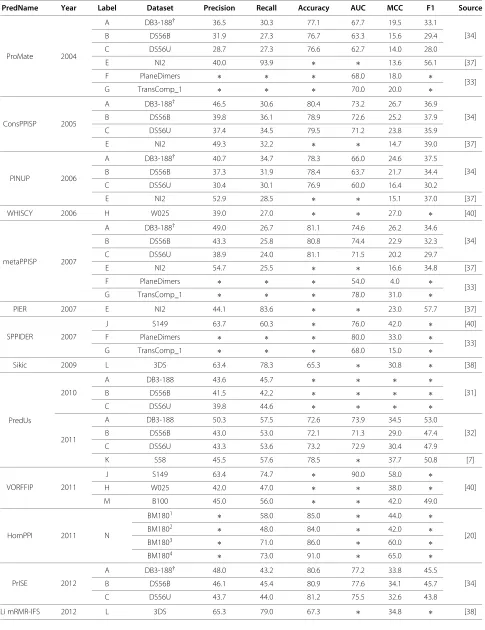
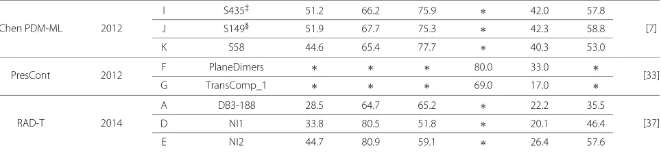
A comparative evaluation of PPIS predictors has been per-formed in previous reviews [109,214]; as such, we focus on information regarding only the most recent predictors, shown in Table 4.
Objective evaluation of PPIS predictor performance is made difficult by the varying definitions of interaction sites and accessible surface residues in the literature, the lack of available servers for all predictors, the adoption of varying training and testing datasets, and the different metrics used for evaluation [4,47]. We partially circum-vent these problems by considering the performance of each predictor across a variety of test sets based on litera-ture values.
Assessment measures
PPIS predictors are generally judged with a number of standard performance metrics, including sensitivity (recall, true positive rate, or coverage), precision, and specificity:
Accuracy = TP+TN
TP+FP+TN+FN
Precision = TP
TP+FP
Sensitivity = TP TP+FN
Specificity = TN
TN+FP
whereTP,TN,FP, andFN denote true and false positives and negatives, respectively.
Measures designed to balance between false negative and positive rates includeF1and MCC [219]:
F1=2 precision·recall
precision+recall
MCC= TP·TN−FP·FN α where:
α=(TP+FP)(TP+FN)(TN+FP)(TN+FN) Similarly, the receiver operator curve (ROC), which is a plot of sensitivityversus 1−specificityderived by vary-ing the classifier prediction threshold, can be used to compute the area under the ROC curve (AUROC/AUC) [251], which is especially useful for identifying artifi-cially “inflated” performance (e.g. higher sensitivity at the expense of specificity) and for being decision threshold independent [252].
In general, similar to the lack of consensus in interface definitions and datasets, there is no standard criteria for performance assessment [47]. Given that some false posi-tive predictions may be correct (due to the paucity of crys-tallized complexes), patch-specific performance metrics (i.e. assessing the correct answer in a local patch around an interface in question, such as by the Sørensen-Dice index [253,254]) may be used, though this poorly accounts for false positives. While other evaluation methods have been devised [16,35], computing the statistics above per residue and averaging across the dataset appears to be the most objective and easily comparable method.
The authors note that even the more balanced measures should not be solely relied on (e.g. MCC may favour over-prediction in PPIS over-prediction [214] and underover-prediction elsewhere [255]) and that predictor performance should be viewed holistically across as many metrics as possible, as balancing performance metrics is domain-dependent [47,255]. When considering PPIS prediction for mimetic drug design, slight underprediction may be desirable, as it will likely find the better discriminated core residues [7,33], from which the remaining PPIS can be inferred (rather than “guessing” which of many allegedly “active” residues is even interacting).
Comparative evaluation
Table 4 Comparative evaluation of recent predictors
PredName Year Label Dataset Precision Recall Accuracy AUC MCC F1 Source
ProMate 2004
A DB3-188† 36.5 30.3 77.1 67.7 19.5 33.1
[34]
B DS56B 31.9 27.3 76.7 63.3 15.6 29.4
C DS56U 28.7 27.3 76.6 62.7 14.0 28.0
E NI2 40.0 93.9 ∗ ∗ 13.6 56.1 [37]
F PlaneDimers ∗ ∗ ∗ 68.0 18.0 ∗
[33]
G TransComp_1 ∗ ∗ ∗ 70.0 20.0 ∗
ConsPPISP 2005
A DB3-188† 46.5 30.6 80.4 73.2 26.7 36.9
[34]
B DS56B 39.8 36.1 78.9 72.6 25.2 37.9
C DS56U 37.4 34.5 79.5 71.2 23.8 35.9
E NI2 49.3 32.2 ∗ ∗ 14.7 39.0 [37]
PINUP 2006
A DB3-188† 40.7 34.7 78.3 66.0 24.6 37.5
[34]
B DS56B 37.3 31.9 78.4 63.7 21.7 34.4
C DS56U 30.4 30.1 76.9 60.0 16.4 30.2
E NI2 52.9 28.5 ∗ ∗ 15.1 37.0 [37]
WHISCY 2006 H W025 39.0 27.0 ∗ ∗ 27.0 ∗ [40]
metaPPISP 2007
A DB3-188† 49.0 26.7 81.1 74.6 26.2 34.6
[34]
B DS56B 43.3 25.8 80.8 74.4 22.9 32.3
C DS56U 38.9 24.0 81.1 71.5 20.2 29.7
E NI2 54.7 25.5 ∗ ∗ 16.6 34.8 [37]
F PlaneDimers ∗ ∗ ∗ 54.0 4.0 ∗
[33]
G TransComp_1 ∗ ∗ ∗ 78.0 31.0 ∗
PIER 2007 E NI2 44.1 83.6 ∗ ∗ 23.0 57.7 [37]
SPPIDER 2007
J S149 63.7 60.3 ∗ 76.0 42.0 ∗ [40]
F PlaneDimers ∗ ∗ ∗ 80.0 33.0 ∗
[33]
G TransComp_1 ∗ ∗ ∗ 68.0 15.0 ∗
Sikic 2009 L 3DS 63.4 78.3 65.3 ∗ 30.8 ∗ [38]
PredUs
2010
A DB3-188 43.6 45.7 ∗ ∗ ∗ ∗
[31]
B DS56B 41.5 42.2 ∗ ∗ ∗ ∗
C DS56U 39.8 44.6 ∗ ∗ ∗ ∗
2011
A DB3-188 50.3 57.5 72.6 73.9 34.5 53.0
[32]
B DS56B 43.0 53.0 72.1 71.3 29.0 47.4
C DS56U 43.3 53.6 73.2 72.9 30.4 47.9
K S58 45.5 57.6 78.5 ∗ 37.7 50.8 [7]
VORFFIP 2011
J S149 63.4 74.7 ∗ 90.0 58.0 ∗
[40]
H W025 42.0 47.0 ∗ ∗ 38.0 ∗
M B100 45.0 56.0 ∗ ∗ 42.0 49.0
HomPPI 2011 N
BM1801 ∗ 58.0 85.0 ∗ 44.0 ∗
[20]
BM1802 ∗ 48.0 84.0 ∗ 42.0 ∗
BM1803 ∗ 71.0 86.0 ∗ 60.0 ∗
BM1804 ∗ 73.0 91.0 ∗ 65.0 ∗
PrISE 2012
A DB3-188† 48.0 43.2 80.6 77.2 33.8 45.5
[34]
B DS56B 46.1 45.4 80.9 77.6 34.1 45.7
C DS56U 43.7 44.0 81.2 75.5 32.6 43.8
Table 4 Comparative evaluation of recent predictors(Continued)
Chen PDM-ML 2012
I S435‡ 51.2 66.2 75.9 ∗ 42.0 57.8
[7]
J S149§ 51.9 67.7 75.3 ∗ 42.3 58.8
K S58 44.6 65.4 77.7 ∗ 40.3 53.0
PresCont 2012 F PlaneDimers ∗ ∗ ∗ 80.0 33.0 ∗ [33]
G TransComp_1 ∗ ∗ ∗ 69.0 17.0 ∗
RAD-T 2014
A DB3-188 28.5 64.7 65.2 ∗ 22.2 35.5
[37]
D NI1 33.8 80.5 51.8 ∗ 20.1 46.4
E NI2 44.7 80.9 59.1 ∗ 26.4 57.6
†refers to the DB3-188 set excluding 2VIS;‡refers to the S435 set excluding 3 proteins due to obsolescence or absence;§refers to the S149 set excluding 7 proteins
due to existence in training set. BM1801are transient enzyme-inhibitor complexes, BM1802are transient non-enzyme- inhibitor complexes, BM1803are obligate hetero-dimers and BM1801are obligate homo-dimers.
intrinsically more predictable, as evidenced by higher scores across all predictors; others achieve better results only on certain types of predictors (e.g. DB3-188 on struc-tural homology-based predictors). To achieve high scores on specialized testing datasets, predictors often require either specializations of their own, or inherent character-istics that permit accurate classification (e.g. ANCHOR’s [10] specialization for disordered proteins and HomPPI’s [20] lack of requirement for structural information allow them both to successfully predict on the S1/2 disordered sets). Theoretically, unbound structures are more diffi-cult to predict on than bound monomers (due to the conformational disparity between the two sets); this is largely confirmed by differing results on the DS56B/U sets, as well as generally lower scores on unbound sets (Table 4). Overall, we find that there has been signifi-cant progress in the predictive abilities of the predictors over the last decade across diverse interaction types and datasets.
Future directions
Though the field of PPIS prediction has been steadily improving in accuracy and sophistication over time, chal-lenges remain before scores sufficient to permit its many potential applications can be achieved.
Accounting for interface type and subclass
The classification of interfaces between transient, per-manent, and obligate, as well as within interfaces as core and rim structures, has been extensively studied from a theoretical standpoint. However, with some excep-tions [20,33,52], this information has been algorithmically underutilized for PPIS prediction. Focusing on datasets of a particular complex type, combining interface classi-fication with interaction likelihood prediction, and inte-grating learning of the different properties of the interface core and rim into PPIS prediction are just a few examples of promising areas that are currently under investigation.
Closer examination of datasets
As with much biological data, protein structural datasets are non-standardized and virtually all structure-based predictors have varying criteria for processing and fil-tering this data. The types of proteins that are the least predictable, or the difference between large but hetero-geneous training sets versus smaller but cleaner ones, have not been comprehensively examined. Specialized training sets per query protein, whether by structural, sequence-level, or functional data, are worth exploring as well. Potentially, unsupervised learning could be applied to extract hidden patterns within the data, possibly con-tributing to further analysis of the relation between inter-action types, protein categories, and the feature space. Further, methods accounting for systemic biases in the PDB (e.g. under-representation of membrane/disordered proteins) may also improve robustness [256,257].
Improved benchmarking
More comprehensive and standardized benchmarking, as noted in other reviews [75], is essential to advancing the field. Additionally, to facilitate comparative evaluation of performance, as well as to ensure that improvements are not statistical anomalies, the authors suggest that signifi-cance testing be applied to future published work.
Utilizing ensemble approaches
predict exceedingly well when homologues are available but fail otherwise, could be combined with a more gen-eral, machine-learning based predictor to complement it in cases where homology information is missing. On a smaller scale, ensemble methods utilizing a set of predic-tors (e.g. residue-specific [42], atom-specific [7], bagging-based [7]) appear to be useful for reducing noise and making better use of the available information contained within the protein.
Integrating other areas of computational biology
Greater integration of PPIS prediction with other areas of computational biology also holds promise. The relatively small number of crystallized structures suggests PPIS pre-dictions based on structural characteristics may not be helpful when such information is not present; however, the use of molecular modeling could prove useful in miti-gating this problem. Other areas of bioinformatics are also being applied to assist PPIS prediction, such as molecular docking [11,19,53,260].
Further application of computational techniques
Several areas of PPIS prediction could benefit from the use of more sophisticated computational learning techniques. For feature selection and extraction, current methods can be combined (e.g. MRMR or PCA with GRS) or extended (e.g. empirical Bernstein bounds [261] with GRS, non-linear component analysis [262], or autoencoders [263]). The class imbalance problem has been recently circum-vented via bagging [7], but semi-supervised learning could also be applied, as seen for hotspot [264,265] and pair-wise protein interaction prediction [266], with minimal changes to the features used. Indeed, as “non-interacting” residues may be mislabelled (since every possible protein complex is certainly not known), semi-supervised learn-ing methods for handllearn-ing this problem are even more applicable [267,268].
Recently, methods for accounting for neighbourhood information have become more prevalent, including averaging across the local environment [7,33], Voronoi diagrams [40], and feature concatenation [8,38], each pro-viding gains in predictive ability. This suggests that meth-ods for multi-scale machine learning could prove effective [258,259]. Machine learning techniques for multi-class classification [269,270] (e.g. separating core vs. rim vs. surface) also hold potential for improvement.
Applications
The identification of interacting residues on protein sur-faces holds potential for use in diverse fields across biology and medicine. One of the most related problems is the elucidation of the residues inside PPISs that account for the major change in free binding energy upon complex formation, known as hotspots (HSs) [271,272]. ML-based
PPIS predictors have already been successfully used for HS prediction by simply altering the training set [161]. Interface predictions may be used to narrow the search space of HS predictors, as HSs tend to localize to the interface core [33,273]. For the same reason, putative HS residues could be used to “seed” interface site predictions. Similarly, knowledge of a PPIS can be used to guide muta-genesis experiments to more promising sites, reducing the expense and time required for a whole-protein analysis.
Most importantly, knowledge of PPISs and HSs can be used for rational design of therapeutics and biomolecules by serving as a template for thede novocreation of small molecules with enhanced efficacy and selectivity. Mimet-ics of the interaction sites of well-known molecules have been successfully built [274,275], the process of which could be significantly expedited by the knowledge of putative interaction sites, as it would allow rational con-struction of a mimetic compound without requiring mass screening. The design of novel interface sites has also shown promise for the construction of new functional biomolecules [276,277].
Another interesting application is in assisting compu-tational protein-protein docking. Docking without prior knowledge of the interaction sites of the proteins in ques-tion (i.e.ab initiodocking) has been shown to be more difficult due to the staggering search space dimension-ality involved [278]. Information-driven docking [279] can mitigate this problem by utilizing mass spectroscopy and interaction data, the latter of which is often diffi-cult to obtain, but can be provided by PPIS prediction. This approach has already proven successful in both high-resolution docking [17,24,41] and coarse mass docking experiments [280]. Additionally, PPIS-driven coarse dock-ing studies could assist in large-scale PPI network creation [281], as well as alignment of such networks for functional ortholog identification [282-284].
Conclusion
believe that future advances will bring predictors capable of significantly contributing to biomedical and pharma-ceutical science.
Competing interests
The authors declare that they have no competing interests.
Authors’ contributions
All authors planned, researched, and wrote the paper. All authors read and approved the final manuscript.
Author details
1Department of Anatomy and Cell Biology, McGill University, Montreal, Canada.2School of Computer Science, McGill University, Montreal, Canada. 3Department of Microbiology and Immunology, McGill University, Montreal, Canada.
Received: 23 August 2014 Accepted: 7 January 2015
References
1. Krüger DM, Gohlke H. Drugscoreppi webserver: fast and accurate in silico alanine scanning for scoring protein–protein interactions. Nucleic Acids Res. 2010;38(suppl 2):480–6.
2. Bradshaw RT, Patel BH, Tate EW, Leatherbarrow RJ, Gould IR. Comparing experimental and computational alanine scanning techniques for probing a prototypical protein–protein interaction. Protein Eng Des Sel. 2011;24(1-2):197–207.
3. Aloy P, Russell RB. Ten thousand interactions for the molecular biologist. Nat Biotechnol. 2004;22(10):1317–21.
4. Porollo A, Meller J. Computational methods for prediction of protein-protein interaction sites. Protein-Protein Interactions-Computational and Experimental Tools; W. Cai and H. Hong, Eds. InTech. 2012;472:3–26. 5. Jones S, Thornton JM. Analysis of protein-protein interaction sites using
surface patches. J Mol Biol. 1997;272(1):121–32.
6. Jones S, Thornton JM. Prediction of protein-protein interaction sites using patch analysis. J Mol Biol. 1997;272(1):133–43.
7. Chen C-T, Peng H-P, Jian J-W, Tsai K-C, Chang J-Y, Yang E-W, et al. Protein-protein interaction site predictions with three-dimensional probability distributions of interacting atoms on protein surfaces. PloS one. 2012;7(6):37706.
8. Šiki´c M, Tomi´c S, Vlahoviˇcek K. Prediction of protein–protein interaction sites in sequences and 3d structures by random forests. PLoS Comput Biol. 2009;5(1):1000278.
9. Fiorucci S, Zacharias M. Prediction of protein-protein interaction sites using electrostatic desolvation profiles. Biophys J. 2010;98(9):1921–30. 10. Dosztányi Z, Mészáros B, Simon I. Anchor: web server for predicting
protein binding regions in disordered proteins. Bioinformatics. 2009;25(20):2745–6.
11. Martin J, Lavery R. Arbitrary protein- protein docking targets biologically relevant interfaces. BMC Biophys. 2012;5(1):7.
12. La D, Kihara D. A novel method for protein–protein interaction site prediction using phylogenetic substitution models. Proteins: Struct Funct Bioinform. 2012;80(1):126–41.
13. Bradford JR, Westhead DR. Improved prediction of protein–protein binding sites using a support vector machines approach. Bioinformatics. 2005;21(8):1487–94.
14. Chen X-W, Jeong JC. Sequence-based prediction of protein interaction sites with an integrative method. Bioinformatics. 2009;25(5):585–91. 15. Chung J-L, Wang W, Bourne PE. Exploiting sequence and structure
homologs to identify protein–protein binding sites. Proteins: Struct Funct Bioinform. 2006;62(3):630–40.
16. Chen H, Zhou H-X. Prediction of interface residues in protein–protein complexes by a consensus neural network method: test against nmr data. Proteins: Struct Funct Bioinform. 2005;61(1):21–35.
17. de Vries SJ, Bonvin AM. Cport: a consensus interface predictor and its performance in prediction-driven docking with haddock. PLoS One. 2011;6(3):17695.
18. Dong Q, Wang X, Lin L, Guan Y. Exploiting residue-level and profile-level interface propensities for usage in binding sites prediction of proteins. BMC Bioinform. 2007;8(1):147.
19. Fernández-Recio J, Totrov M, Abagyan R. Identification of
protein–protein interaction sites from docking energy landscapes. J Mol Biol. 2004;335(3):843–65.
20. Xue LC, Dobbs D, Honavar V. Homppi: a class of sequence homology based protein-protein interface prediction methods. BMC Bioinform. 2011;12(1):244.
21. Shoemaker BA, Zhang D, Thangudu RR, Tyagi M, Fong JH,
Marchler-Bauer A, et al. Inferred biomolecular interaction server—a web server to analyze and predict protein interacting partners and binding sites. Nucleic Acids Res. 2009;38:842.
22. Ofran Y, Rost B. Isis: interaction sites identified from sequence. Bioinformatics. 2007;23(2):13–6.
23. Engelen S, Trojan LA, Sacquin-Mora S, Lavery R, Carbone A. Joint evolutionary trees: a large-scale method to predict protein interfaces based on sequence sampling. PLoS Comput Biol. 2009;5(1):1000267. 24. Huang B, Schroeder M. Using protein binding site prediction to improve
protein docking. Gene. 2008;422(1):14–21.
25. Qin S, Zhou H-X. meta-ppisp: a meta web server for protein-protein interaction site prediction. Bioinformatics. 2007;23(24):3386–7. 26. Tjong H, Qin S, Zhou H-X. Pi2pe: protein interface/interior prediction
engine. Nucleic Acids Res. 2007;35(suppl 2):357–62.
27. Kufareva I, Budagyan L, Raush E, Totrov M, Abagyan R. Pier: protein interface recognition for structural proteomics. Proteins: Struct Funct Bioinform. 2007;67(2):400–17.
28. Liang S, Zhang C, Liu S, Zhou Y. Protein binding site prediction using an empirical scoring function. Nucleic Acids Res. 2006;34(13):3698–707. 29. Li M-H, Lin L, Wang X-L, Liu T. Protein–protein interaction site prediction
based on conditional random fields. Bioinformatics. 2007;23(5):597–604. 30. Zhou H-X, Shan Y. Prediction of protein interaction sites from sequence
profile and residue neighbor list. Proteins: Struct Funct Bioinform. 2001;44(3):336–43.
31. Zhang QC, Petrey D, Norel R, Honig BH. Protein interface conservation across structure space. Proc Nat Acad Sci. 2010;107(24):10896–901. 32. Zhang QC, Deng L, Fisher M, Guan J, Honig B, Petrey D. Predus: a web
server for predicting protein interfaces using structural neighbors. Nucleic Acids Res. suppl 2;39:283–7.
33. Zellner H, Staudigel M, Trenner T, Bittkowski M, Wolowski V, Icking C, et al. Prescont: Predicting protein-protein interfaces utilizing four residue properties. Proteins: Struct Funct Bioinform. 2012;80(1):154–68. 34. Jordan RA, Yasser E-M, Dobbs D, Honavar V. Predicting protein-protein
interface residues using local surface structural similarity. BMC Bioinformatics. 2012;13(1):41.
35. Neuvirth H, Raz R, Schreiber G. Promate: a structure based prediction program to identify the location of protein–protein binding sites. J Mol Biol. 2004;338(1):181–99.
36. Murakami Y, Mizuguchi K. Applying the naïve bayes classifier with kernel density estimation to the prediction of protein–protein interaction sites. Bioinformatics. 2010;26(15):1841–8.
37. Bendell CJ, Liu S, Aumentado-Armstrong T, Istrate B, Cernek PT, Khan S, et al. Transient protein-protein interface prediction: datasets, features, algorithms, and the rad-t predictor. BMC Bioinformatics. 2014;15(1):82. 38. Li B-Q, Feng K-Y, Chen L, Huang T, Cai Y-D. Prediction of protein-protein
interaction sites by random forest algorithm with mrmr and ifs. PloS one. 2012;7(8):43927.
39. Porollo A, Meller J. Prediction-based fingerprints of protein–protein interactions. PROTEINS: Structure Function Bioinform. 2007;66(3):630–45. 40. Segura J, Jones PF, Fernandez-Fuentes N. Improving the prediction of
protein binding sites by combining heterogeneous data and voronoi diagrams. BMC Bioinformatics. 2011;12(1):352.
41. de Vries SJ, van Dijk AD, Bonvin AM. Whiscy: What information does surface conservation yield? application to data-driven docking. Proteins: Struct Funct Bioinform. 2006;63(3):479–89.
42. de Moraes FR, Neshich IA, Mazoni I, Yano IH, Pereira JG, Salim JA, et al. Improving predictions of protein-protein interfaces by combining amino acid-specific classifiers based on structural and physicochemical descriptors with their weighted neighbor averages. PloS One. 2014;9(1): 87107.
43. Qiu Z, Wang X. Prediction of protein–protein interaction sites using patch-based residue characterization. J Theor Biol. 2012;293:143–50. 44. Janin J. Basic principles of protein–protein interaction. Computational