Received: 18 September 2008 – Published in The Cryosphere Discuss.: 25 November 2008 Revised: 28 April 2009 – Accepted: 28 April 2009 – Published: 4 May 2009
Abstract. We have developed a new digital elevation model (DEM) of Antarctica from a combination of satellite radar and laser altimeter data. Here, we assess the accuracy of the DEM by comparison with airborne altimeter data from four campaigns covering a wide range of surface slopes and ice sheet regions. Root mean squared (RMS) differences var-ied from 4.75 m, when compared to a densely gridded air-borne dataset over the Siple Coast region of West Antarctica to 33.78 m when compared to a more limited dataset over the Antarctic Peninsula where surface slopes are high and the across track spacing of the satellite data is relatively large. The airborne data sets were employed to produce an error map for the DEM by developing a multiple linear regression model based on the variables known to influence errors in the DEM. Errors were found to correlate highly with surface slope, roughness and density of satellite data points. Errors ranged from typically∼1 m over the ice shelves to between about 2 and 6 m for the majority of the grounded ice sheet. In the steeply sloping margins, along the Peninsula and moun-tain ranges the estimated error is several tens of metres. Less than 2% of the area covered by the satellite data had an esti-mated random error greater than 20 m.
1 Introduction
Digital elevation models (DEMs) of the Antarctic are impor-tant datasets for a wide range of applications from fieldwork planning, calculating drainage basins, calculating mass bal-ance, determining balance velocities to dynamical modelling of the ice sheet (Budd and Warner, 1996; Remy et al., 1999; Rignot et al., 2008; Smith et al., 2006). The limitations of currently available DEMs (Bamber and Gomez-Dans, 2005)
Correspondence to: J. A. Griggs
and the availability of new, higher quality altimeter data for the Antarctic continent has led us to produce a new DEM. The methodology and data used is described in detail in a companion paper (Bamber et al., 2009) and so we repeat only the most salient points here. The new DEM was created by combining high-accuracy, but relatively low spatial res-olution, laser altimeter data from the GLAS instrument on-board IceSat (Zwally et al., 2007) with radar altimeter data from the geodetic phase of the ERS-1 satellite, which pro-vided dense spatial coverage but lower vertical accuracy par-ticularly in highly sloping areas (Brenner et al., 2007). The ERS-1 data are the same as those used to create an earlier DEM derived solely from radar altimetry (Bamber and Bind-schadler, 1997). The resulting DEM was gridded with 1 km postings.
2 Validation
As mentioned, the accuracy of the new DEM was estimated by comparison with airborne altimeter data. The airborne data had a variable accuracy in the range 0.08–1.91 m de-pending on the campaign. It should be noted that the airborne data measured the surface elevation at a higher spatial resolu-tion than the satellite sensors and so some differences will be due to the airborne data ranging into crevasses and rifts be-low the surface which were not resolved by the spaceborne instruments. In addition, temporal differences between the time stamp of the DEM (2004) and the airborne data (vari-able between 1991 and 2007) must also be considered par-ticularly in areas of fast-flow and known surface elevation change such as Pine Island and Thwaites glaciers (Shepherd et al., 2002) and Kamb Ice Stream (Csatho et al., 2005).
Four airborne datasets were compared to the DEM to as-sess its accuracy. These datasets were
– CECS/NASA over the Antarctic Peninsula and Pine Is-land, Thwaites, Pope, Smith and Kohler glaciers – AGASEA over the Amundsen Sea sector
– SOAR CASERTZ over the south-eastern Ross Embay-ment and
– ISODYN/WISE in northern Victoria Land.
The locations of these data are shown in Fig. 1 and the acronyms explained below. The comparison with the DEM is discussed for each data set, next. In all cases, bilinear in-terpolation was used to calculate the DEM elevation at the exact location of the airborne measurement and differences are calculated in the sense airborne measurement – interpo-lated DEM value. Other interpolation methods are available, such as bicubic splines, but make a negligible difference to the results. The statistics presented are mean and modal dif-ference, standard deviation around the mean difdif-ference, root mean squared (RMS) difference and full width at half max-imum (FWHM), which is a useful measure of error when a distribution is non-Gaussian.
The mean difference expresses the systematic error or bias. The modal difference provides the most common difference and is a secondary measure of the systematic error. As with the FWHM, it can be a more appropriate measure of bias than mean difference when the histogram is non-Gaussian. It also allows direct comparison with Young et al. (2008) who report bias in several older DEMs using this measure only. The final three statistics all measure the random error in the DEM. They are all presented, primarily, to allow comparison with other studies but also because the histograms of differences are not always Gaussian (Bamber and Gomez-Dans, 2005).
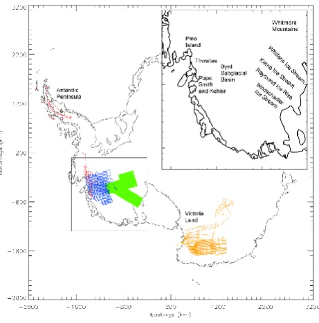
Fig. 1. Validation datasets. Red flight lines indicate the position of the CECS/NASA data, blue flight lines indicate AGASEA data, green flight lines indicate SOAR CASERTZ data and yellow flight lines indicate the position of ISODYN/WISE data. The square box indicates the region shown in the inset. The inset shows the loca-tions of important features referenced in the text in the Amundsen Sea sector.
2.1 CECS/NASA
The CECS/NASA data were collected on a joint Centro de Estudios Cientif´ıos (CECS), Chile and NASA organised sur-vey (Rignot et al., 2004). The areas covered were Pine Island, Thwaites, Pope, Smith and Kohler glaciers in the Amundsen Sea sector and the Antarctic Peninsula. The survey oper-ated from a Chilean P-3 aircraft carrying the NASA/Wallops Airborne Topographic Mapper (ATM) (Krabill et al., 2000). Flights of 750–1000 km length were collected in November and December 2002. The survey operated with a long base-line GPS (∼1400 km) which gave an accuracy of around 20– 30 cm, a factor two worse than that achieved in Greenland where shorter baseline GPS measurements were used.
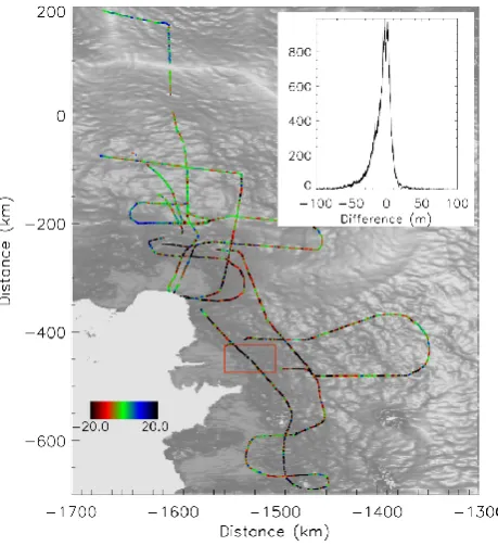
Fig. 2. Difference between the CECS/NASA data and the DEM in the peninsula region overlaid on a shaded relief of the DEM. Inset shows a histogram of the differences.
is an area of the DEM with little satellite data and interpola-tion lengths are long as can be seen from the distribuinterpola-tion of input datapoint in Fig. 4 of Bamber et al. (2009). Over the entire Peninsula region, the difference between the airborne data and the DEM has a mean bias of 1.08 m, modal bias of 0.29 m and RMS difference of 33.78 m.
Figure 3 shows the difference between the CECS/NASA data and the DEM for the Amundsen Sea sector. Here, better agreement is seen than over the Peninsula due to the greater amount of satellite data present in the DEM and the more gentle relief. Over Pine Island glacier and ice shelf, the agreement is better than over Thwaites glacier with a mean difference of−9.63 m±6.98 m compared to a mean differ-ence of−14.08 m±18.13 m for Thwaites. A small section over the centre of Thwaites glacier (indicated by the red box on Fig. 3) shows mean differences of −42.31 m with the DEM being consistently higher than the airborne data as shown in Fig. 4. This is a region, which is believed to be close to, or oceanward of, the 1996 limit of tidal flexure and so is likely on the floating ice tongue of Thwaites glacier (Rignot et al., 2004). The ice tongue surface does not resem-ble a simple ice shelf but is a collection of broken up icebergs attached together by an ice melange of sea ice, ice sheet de-bris and windblown snow (Rignot and MacAyeal, 1998). The ice tongue rifts and calves into large tabular icebergs along a significant proportion of the grounding line (Rignot, 2001). It is therefore likely the airborne data are ranging, in places, to the lower elevation melange and the satellite data to the
Fig. 3. Difference between the CECS/NASA data and the DEM in the Amundsen Sea sector overlaid on a shaded relief of the DEM. Inset shows a histogram of the differences.
Fig. 4. Profile across the mouth of Thwaites glacier showing large difference between airborne data and DEM. Black line shows data from the DEM and grey line is the NASA/CECS data.
Fig. 5. Difference between the AGASEA data and the DEM in the Amundsen Sea sector overlaid on a shaded relief of the DEM. Inset shows a histogram of the differences. Red box shows position of region defined in the text as “central area”.
2.2 AGASEA
The AGASEA (Airborne Geophysical Survey of the Amund-sen Sea Embayment, Antarctica) dataset (Young et al., 2008) was collected by the University of Texas Institute for Geo-physics between 12 December 2004 and 30 January 2005. The data were collected with a 15 km grid spacing over the Thwaites and Smith glacier catchments using a Twin Otter fitted with an ice penetrating radar, gravimeter and magne-tometer in addition to a nadir pointing laser distance me-ter for measuring surface elevation. In addition to flying the grid, targeted profiles were flown reflying three IceSat ground tracks. The laser altimeter configuration results in a 1 m wide ground spot size with an along track resolution of approximately 20 m. Cross-over analysis of the data per-formed by Young et al. (2008) showed an RMS difference for the entire dataset of±20 cm and±8 cm when a reference dataset consisting of datapoints closest to the base reference GPS station was considered. The data exhibited an approx-imately 20 cm bias from the IceSat dataset in flat areas for which the source is unknown (Young et al., 2008). This bias increased to 27 cm when all areas were considered.
Figure 5 shows the difference between the AGASEA air-borne data and DEM along with a histogram of the differ-ences. The agreement between the airborne data and the DEM is highest in flat and low slope areas such as the area marked by the red box where the mean difference is 9 cm±4.68 m. The agreement is poorer in fast flow areas with the coastal region of the dataset having a mean differ-ence of−10.47 m±19.83 m. This area is where crevassing is more prevalent and the surface is much rougher and so
agreement is expected to be poorer due to the difference in spatial resolution of the two types of measurement. This is manifested in differences which are highly variable ex-hibiting both positive and negative differences close to each other. We also note that the DEM may not be able to fully resolve mountains in this region including Mount Takahe (close to x=−1390 km, y=−560 km on Fig. 5) and Mount Frakes (close to x=−1275 km, y=−660 km on Fig. 5) due to their small spatial scale compared to the interpolation length and lack of ERS data in break-in slope regions but there are gaps in the airborne grid at these points so we are unable to determine the DEM’s accuracy. The mean bias observed across the whole dataset is −4.55 m with a modal bias of −0.61 m and an RMS difference of 13.14 m.
2.3 SOAR CASERTZ
The SOAR CASERTZ data (Support Office for Aerogeo-physical Research – Corridor Aerogeophysics of the South East Ross Transect Zone) data were recorded by the Univer-sity of Texas Institute for Geophysics and the US Geological Survey (Blankenship et al., 2001). Flights were conducted over an area encompassing the onset area and catchment region of Whillans and Kamb Ice Streams (formerly, Ice Streams B and C), all of Bindschadler Ice Stream (Ice Stream D) and the boundary between the West Antarctic rift sys-tem and the crustal provinces dominated by Byrd Subglacial Trench and the Whitmore Mountains. Data were recorded in Antarctic summer seasons between 1991 and 1997 using a laser altimeter on a Twin Otter aircraft providing approxi-mately 8 m along track spacing. The instrument was capable of a precision of better than 10 cm in the absence of cloud cover and surface elevation profiles were repeatable to within 25 cm across track. RMS deviations were calculated at cross-over points and values varying between±37 cm for the earli-est seasons, before the full GPS constellation was deployed, to±9 cm for the most recent survey. The data were provided on a 425 m resolution grid.
Fig. 6. Difference between the SOAR CASERTZ data and the DEM in the Siple coast region overlaid on a shaded relief of the DEM. Inset shows a histogram of the differences.
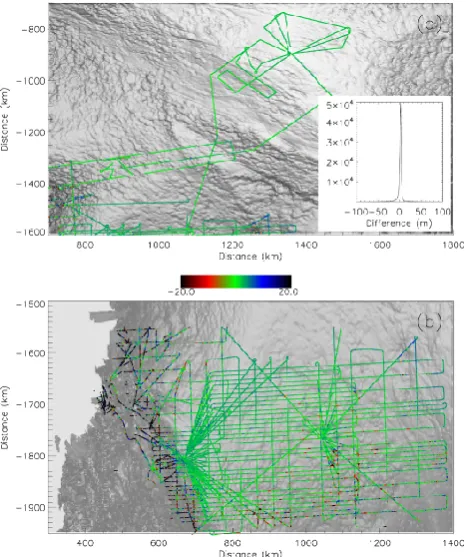
Fig. 7. (a) Difference between the SOAR CASERTZ data and the DEM over Siple Dome. (b) Difference between the SOAR CASERTZ data and an earlier version of the DEM created using a slope based bias correction on the ERS data.
be thickening significantly (Csatho et al., 2005). The size of negative differences between the SOAR CASERTZ data and the DEM are similar to that expected from thickening of up to 0.8 m/yr over the years between the 1991–1997 time stamp of the SOAR CASERTZ data in this region and the 2004 time stamp of the DEM. The mean bias between the airborne data and the DEM for the entire dataset is 0.21 m with a modal difference of 1.97 m and an RMS difference of 4.75 m.
The agreement between the DEM and airborne data on Siple Dome supports the use of the new surface roughness based bias correction applied to the ERS data (Bamber et al., 2009). This was one of the regions where applying a bias correction calculated from slope as a proxy for surface roughness was ineffective, as the surface of Siple Dome is
Fig. 8. Difference between the ISODYN/WISE data and the DEM in northern Victoria Land overlaid on a shaded relief of the DEM. Inset shows a histogram of the differences.
highly sloping yet surface roughness is low (i.e. the second derivative of height is small). A surface slope bias correction was applied in earlier versions of the new DEM (Bamber and Gomez-Dans, 2005). Figure 7 shows the difference between the SOAR CASERTZ data and both the current DEM and an earlier version which uses a surface slope based bias cor-rection. The improved agreement in this region justifies the more physically realistic bias correction to the ERS data. 2.4 ISODYN/WISE
Table 1. Statistics of the comparisons between the DEM and each airborne dataset.
Number of airborne Number of DEM Mean bias Modal bias Standard deviation RMS difference FWHM
datapoints gridboxes (m) (m) (m) (m) (m)
CECS/NASA peninsula 98781 7964 1.08 0.29 33.77 33.78 2.2
CECS/NASA Amundsen 200974 8959 −7.42 −2.05 16.31 17.92 14.1
AGASEA 1672797 37674 −4.55 −0.61 12.33 13.14 11.7
AGASEA (central area)
138077 3024 0.09 1.35 4.68 4.68 3.9
SOAR CASERTZ 1615531 285894 0.21 1.97 4.74 4.75 4.5
ISODYN/WISE 2176824 96487 1.64 2.38 9.69 9.83 3.3
ISODYN/WISE (elevations over 2200m)
912235 40815 2.78 2.76 5.60 6.25 3.3
Table 2. Statistics of the comparison between the AGASEA airborne data and a selection of available Antarctic DEMs. Results from the older DEMs are all taken from Young et al. (2008).
Bias whole area RMS whole area Bias central area RMS central area
(m) (m) (m) (m)
New DEM −0.6 13.2 1.27 4.69
ERS-1 DEM −1.4 27.4 −0.46 5.2
RAMP DEM 0.4 55 1.07 5.7
IceSat DEM −0.2 18.4 0.4 4.4
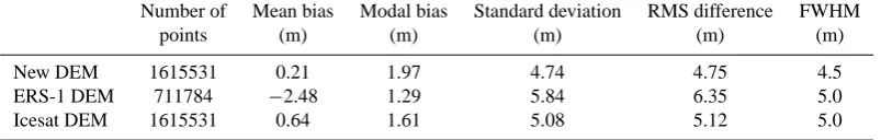
Table 3. Statistics of the comparison between the SOAR CASERTZ airborne data and a selection of available Antarctic DEMs.
Number of Mean bias Modal bias Standard deviation RMS difference FWHM
points (m) (m) (m) (m) (m)
New DEM 1615531 0.21 1.97 4.74 4.75 4.5
ERS-1 DEM 711784 −2.48 1.29 5.84 6.35 5.0
Icesat DEM 1615531 0.64 1.61 5.08 5.12 5.0
DEM and a mean bias of 2.78 m with an RMS difference of 6.25 m when comparing just those datapoints with elevation over 2200 m.
3 Comparison to other available DEMs
The results of the comparison of the DEM with the 5 inde-pendent airborne altimetry datasets are shown in Table 1. The accuracy and random error in the new DEM is within expec-tations given data accuracy and coverage in most areas, wors-ening in areas of steeper relief and poorer satellite coverage. To put these results in context, we have compared them with other DEMs of Antarctica. The AGASEA dataset have been compared with the RAMP (Liu et al., 1999), ERS-1 (Bamber and Bindschadler, 1997) and IceSat (DiMarzio et al., 2007) DEMs in a previous study (Young et al., 2008). A bicubic in-terpolation scheme was used to interpolate the DEMs to the
location of the airborne data. This, however, makes a negli-gible difference to the statistics of the differences when com-pared with the bilinear interpolation used here. The results from the earlier study along with those from the compari-son of our new DEM are given in Table 2, for the AGASEA data set using the bicubic interpolation method and the modal measure of bias. Values are shown for both the entire area as well as for a central, plateau area, highlighted by the red box on Fig. 4. The RMS difference for the whole area is lowest for the new DEM and around 6.5% higher than the ICESat DEM for the plateau region.
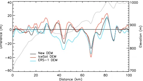
difference to the new DEM, red shows the difference to the IceSat DEM and blue shows the difference to the ERS-1 DEM. Elevation of the SOAR CASERTZ dataset along the profile is plotted as a dotted line with scale on the right-hand ordinate.
ERS-1 data. Table 3 shows the results of this comparison. In the case of the ERS-1 DEM, we only make a compari-son in areas north of 81.5◦S as, south of this latitude, the DEM was created using cartographic data with accuracy con-siderably poorer than elsewhere (Bamber and Gomez-Dans, 2005). Not surprisingly, the new DEM has a lower RMS and standard deviation compared with the ERS-1 DEM but also compared to the ICESat DEM, although the differences here are on the order of 35 cm, equivalent to∼7%. However, some small scale features on the surface are still not fully captured as seen by the pattern of alternating positive and negative differences in Fig. 6. A profile of the differences between the SOAR CASERTZ data and the DEMs, along the track shown in white on Fig. 6, is plotted in Fig. 9. All the DEMs are missing small scale features at the scale of∼5 km. The reason for this in the new DEM may be due to the inter-polation methodology used or, in the case of the ERS input data which is widespread in this region, the size of the instru-ment footprint (∼4 km) being on a similar scale to the size of the missing features.
4 Error map
The validation shows the quality of the DEM in the selected areas where airborne data exist. These data are, however, limited in spatial extent and so to provide complete informa-tion on the error inherent in the DEM, we use the results of these comparisons to derive an error map for the new DEM. Our implicit assumption is that differences are pre-dominantly due to errors in the DEM. In other words, i) we neglect errors in the airborne data, ii) we ignore the effect of differences in spatial resolution and iii) assume that there are sufficient airborne validation data to fully characterise the er-rors in the DEM. The erer-rors in the airborne data have been
A multiple regression model states that the mean of the re-quired variable,Y, in this case the RMS error in the DEM, can be expressed as a linear combination of thekdependent variables, Xl(l=1, 2,..., k) for all n points in our airborne
study regions. The multiple regression model is expressed as
Yi =a0+
k X
l=1
alXli+Ei (1)
whereEifori=1,...,nare zero mean, independent identically
distributed, random errors in the multiple regression and
a0, a1, ..., akare unknown model parameters. The validation
data could be used to ascertain the values ofa0, a1, ..., ak as long as the validation data covered the full range of values of the dependent variables. The model could then be applied to the whole of Antarctica to create a map of RMS error. The airborne datasets used in the model were the full AGASEA and SOAR CASERTZ datasets and the ISODYN/WISE data from elevations over 2200 m. The data were chosen to in-clude the best quality airborne data over the widest range of surface slopes and type. The modelled parameter was the random error, measured by the RMS difference due to the non-Gaussian nature of the observed differences, as biases have been shown in the earlier section to be small and not spatially coherent. The RMS error was calculated from all the differences between the airborne data and the DEM in each DEM gridbox containing airborne data. RMS errors were calculated from 4 or more differences for 98.5% of dat-apoints. To determine the range of dependent variables,Xl
which contribute significant variance were included in the full model. The full set of dependent variables were:
1. Surface slope (X1). ERS data contained a surface slope bias which was removed but random error in the ERS data has been shown to increase as a function of in-creasing surface slope. The pointing accuracy of IceSat is 1 arcsec (Schutz et al., 2005) which will give an in-creasing large error in elevation for inin-creasing surface slope with a 2◦slope having an error of 10 cm.
2. Surface roughness (X2). ERS data contain a surface roughness bias as they range to the tops of undulations in the surface. The mean bias was removed but a ran-dom component may remain.
3. Number of datapoints (X3). Increasing numbers of satellite datapoints within each DEM gridbox decreases the random error on the measurement of the elevation in that gridbox.
4. Standard deviation (X4). The standard deviation of all satellite datapoints within each DEM gridbox gives an approximate measure of the error and variance in eleva-tion within a grid cell.
5. Deviation from the quasi-regular grid (X5). All satel-lite datapoints were averaged to a quasi-regular grid be-fore being interpolated to the regular 1 km grid of the final DEM. The absolute difference between the eleva-tion in each quasi-regular gridbox and the elevaeleva-tion in those gridboxes in the DEM gives a measure of the error introduced by the use of an interpolation method which produces a smooth surface by allowing the interpolation surface to deviate from the input data.
6. Distance to real datapoint (X6). The further any interpo-lated DEM gridbox was from one which contains satel-lite data then the larger the effect of the interpolation of the satellite data will be and the greater the chance of missing true changes in the surface elevation.
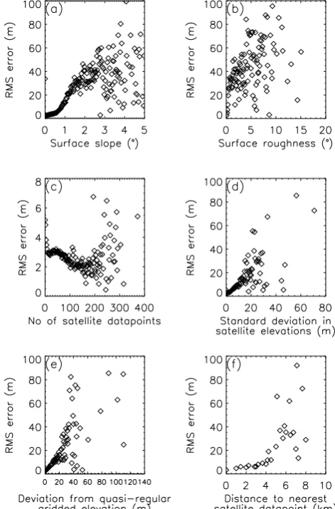
Figure 10 shows plots of the dependent variables against the RMS error calculated from the difference between the air-borne data and the DEM. All dependent parameters were binned into 200 equally sized bins over the full range of val-ues shown. The RMS error is correlated with all dependent variables. At high values of all dependent variables, scatter increases, however, few datapoints exist and this contributes to uncertainty in the regression model as expressed byEi.
The full set of dependent parameters produce a regression model of the form
Y =1.672+3.952X1+8.132X2
−0.019X3+0.033X4+0.345X5+1.051X6 (2) The model was tested to ensure that a regression relation ex-isted by testing the null hypothesis that all regression coeffi-cients were equal to zero. The relation was significant at less
Fig. 10. Plots of the dependent variables in the multiple regression model against the RMS error in the DEM. (a) shows surface slope, (b) shows surface roughness, (c) shows the number of satellite dat-apoints, (d) shows the standard deviation of the satellite datapoints within each DEM gridbox, (e) shows the deviation of the interpo-lated surface from the mean satellite datapoints in each gridbox and (f) shows the distance from each gridbox to the nearest one contain-ing satellite data.
than the 0.1% level. The dependent parameter which con-tributed the least variance to the model wasX4, the standard deviation of satellite datapoints within each DEM gridbox. However, the parameter contributed significant variance to the model at the 99% confidence level and so no dependent variable could be eliminated from the model and Eq. (2) is the full regression model for the RMS error in the DEM.
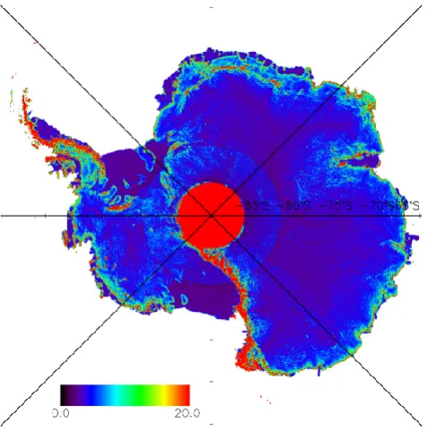
Fig. 11. Map of the distribution of RMS error in the DEM calcu-lated using a multiple regression based on airborne validation data.
increasing over mountainous regions, but remaining less than 25% of the size of the error in all areas apart from those with the very lowest value of RMS error and the highest slope, data-free, mountainous regions. This justifies our third as-sumption in using this method to create an error estimate for our DEM.
The regression model was applied to all DEM gridboxes north of 86◦S. South of this limit, there were no satellite data and the DEM was filled with cartographic data as de-scribed in Bamber et al. (2009). These data do not have the same properties as the satellite derived areas. In the areas of cartographic data, a value of the RMS error was calculated as the RMS difference between the DEM and cartographic data from the same source in a latitude band between 81.5◦S and 86◦S. The error in the area south of 86◦S was found to be 77.09 m. We also limit the maximum size of the error from the regression model to this value. This threshold is ap-plied in some mountainous regions, coastal areas with large interpolation lengths and in some parts of the Peninsula, ac-counting for less than 1% of all gridboxes.
Figure 11 shows the calculated value of RMS error across the whole Antarctic continent. The figure has a range of 0 to 20 m but larger values exist in coastal areas, particu-larly in the Peninsula, where little satellite data exist, and the amount of interpolation present in the DEM was larger than elsewhere. The pattern of RMS error calculated from the re-gression model is as would be expected with errors of around 1–2 m on the ice shelves, where the instruments are known to perform well, surface slopes and roughness are minimal, and spatial sampling is almost complete. The error increases
Fig. 12. Histogram of the distribution of RMS error in the DEM calculated using a multiple regression based on airborne validation data.
slightly on the Ross and Filchner-Ronne ice shelves south of 81.5◦S, moving from an area close to the orbital limit of ERS with very dense satellite coverage to an area with only GLAS data and poorer coverage. RMS errors over the vast majority of the ice sheet interior, covering the high elevation plateaus of East and West Antarctica range between 2 and 6 m. Around the steeper sloping margins, away from moun-tainous areas, the errors are in range 15 to∼40 m (the green-red “rim” in Fig. 11). Figure 12 shows the histogram of the RMS errors, excluding the region south of 86◦S. Around 81% of the DEM has an RMS error less than 5 m and 91% less than 10 m. 98% of the DEM has an error less than 40 m with the remaining gridboxes with higher errors mainly con-fined to mountains, the Peninsula and some isolated points on the coast with steep slopes and therefore, poorer ERS cover-age. Errors on the order of 10 m can be seen around grounded regions in the ice shelves such as Berkner Island and Roo-sevelt Island. These are break-in slope regions where ERS data were not available. 42% of the DEM has an error of 2 m or less, emphasising the strenuous quality assessment per-formed on both satellite datasets.
for mass budget calculations. For such an application, errors in mass flux are directly proportional to errors in thickness and, thus, surface elevation. Similarly, when using the DEM to remove the topographic signal from repeat-pass synthetic aperture radar interferograms, elevation errors have a direct impact on the accuracy of the derived velocities (Joughin et al., 1996). For a meaningful comparison with other topo-graphic data sets, either past or future, and, in particular, for the purposes of determining elevation change over time, an estimate of both the systematic and random errors in the DEM is essential (Paterson and Reeh, 2001). Thus, we be-lieve that the error map significantly enhances the utility and value of the DEM.
5 Conclusions
In Part 1, a new DEM of Antarctica was presented. Airborne validation of this new DEM showed low biases and random errors. Biases are shown to close to zero for all surface slopes surveyed with random errors being about half those from older DEMs based on ERS data only (Bamber and Gomez-Dans, 2005) and between 7 and 30% smaller than those for the DEM containing only GLAS data. When compared to the most widespread airborne dataset (SOAR CASERTZ), which covers a range of surface slope and roughness, a bias of 21cm and random error of 4.75 m are seen. These errors can be partially explained by known changes in the surface over the time period between the recording of the airborne data and the time stamp of the DEM such as the thickening of the stagnant Kamb ice stream.
Using a stepwise multiple regression model, we have cre-ated, what we believe to be, the first rigorous error map to accompany a large scale DEM of Antarctica. Multiple re-gression modelling showed that all six parameters considered have a significant effect on the RMS error of the DEM and all were, therefore, included in the model. These parameters were surface slope, surface roughness, number of satellite datapoint in gridbox, standard deviation of those datapoints, deviation of the interpolated surface from the mean of the satellite datapoints and the distance of an interpolated grid-box to the closest satellite data. The error map shows the expected pattern of low error on smooth, flat surfaces such as the ice shelves and in areas over sub-glacial lakes, with increasing error with increasing slope and surface roughness and in regions with less satellite data. Based on the error map, 81% of the DEM has an RMS error less than 5 m. The error map will allow greater insight into the accuracy of any products derived from it than is currently possible for other DEMs where no such error analysis has been under-taken. It also means that the user can determine if any post-processing, for example, to reduce the resolution, is neces-sary for their application in any given region. Both the DEM and error map will be made available through the National Snow and Ice Data Center for long-term archival.
Acknowledgements. The authors would like to thanks the follow-ing data contributors: W. Krabill from NASA Goddard Wallops Flight Facility for the CECS/NASA data, Duncan Young from the University of Texas for the AGASEA data and Hugh Corr from the British Antarctic Survey for the ISODYN/WISE data. The SOAR data are based on work supported by the National Science Foundation under Grants: OPP-9120464, 9319369 and 9319379 and we’d like to thank SOAR and the University of Texas for allowing us access. This work was funded by NERC grant NE/E004032/1. We would like to thank Stephen Dery, Julian Scott and two anonymous referees for their comments and improvements to the paper.
Edited by: S. Dery
References
Bamber, J. and Gomez-Dans, J. L.: The accuracy of digital eleva-tion models of the Antarctic continent, Earth Planet. Sci. Lett., 237, 516–523, 2005.
Bamber, J. L. and Bindschadler, R. A.: An improved elevation dataset for climate and ice-sheet modelling: validation with satel-lite imagery, Ann. Glaciol., 25, 439–444, 1997.
Bamber, J. L., Gomez-Dans, J. L., and Griggs, J. A.: A new 1 km digital elevation model of the Antarctic derived from combined satellite radar and laser data – Part 1: Data and methods, The Cryosphere, 3, 101–111, 2009,
http://www.the-cryosphere-discuss.net/3/101/2009/.
Blankenship, D. D., Morse, D., Finn, C. A., Bell, R. A., Peters, M. E., Kempf, S. D., Hodge, S. M., Studinger, M., Behrendt, J. C., and Brozena, J. M.: Geologic controls on the initiation of rapid basal motion for West Antarctic ice streams: A geophysi-cal perspective including new airborne radar sounding and laser altimetry results, in: The West Antarctic Ice Sheet, Behavior and Environment, edited by: Alley, R. B. and Bindschadler, R. A., American Geophysical Union, 105–121, 2001.
Brenner, A. C., DiMarzio, J. R., and Zwally, H. J.: Precision and accuracy of satellite radar and laser altimeter data over the continental ice sheets, IEEE T. Geosci. Remote, 45, 321–331, doi:310.1109/TGRS.2006.887172, 2007.
Budd, W. F. and Warner, R. C.: A computer scheme for rapid cal-culations of balance-flux distributions, Ann. Glaciol., 23, 21–27, 1996.
Csatho, B., Ahn, Y., Yoon, T., van der Veen, C. J., Vogel, S., Hamil-ton, G., Morse, D., Smith, B., and Spikes, V. B.: ICESat mea-surements reveal complex pattern of elevation changes on Siple Coast ice streams, Antarctica, Geophys. Res. Lett., 32, L23S04, doi:10.1029/2005GL024289, 2005.
DiMarzio, J. P., Brenner, A. C., Schutz, B. E., Shuman, C. A., and Zwally, H. J.: GLAS/ICESat 500 m laser altimetry digital ele-vation model of Antarctica. Boulder, Colorado, USA. National Snow and Ice Data Center. Digital Media, 2007.
Joughin, I., Kwok, R., and Fahnestock, M.: Estimation of ice-sheet motion using satellite radar interferometry: Method and error analysis with application to Humboldt Glacier, Greenland, J. Glaciol., 42, 564–575, 1996.
Rignot, E.: Evidence for rapid retreat and mass loss of Thwaites Glacier, West Antarctica, J. Glaciol., 47, 213–222, 2001. Rignot, E., Thomas, R. H., Kanagaratnam, P., Casassa, G.,
Freder-ick, E., Gogineni, S., Krabill, W., Rivera, A., Russell, R., Son-ntag, J., Swift, R., and Yungel, J.: Improved estimation of the mass balance of glaciers draining into the Amundsen Sea sector of West Antarctica from the CECS/NASA 2002 campaign, Ann. Glaciol., 39, 231–237, 2004.
Rignot, E., Bamber, J. L., Van Den Broeke, M. R., Davis, C., Li, Y. H., Van De Berg, W. J., and Van Meijgaard, E.: Recent Antarc-tic ice mass loss from radar interferometry and regional climate modelling, Nature Geoscience, 1, 106–110, 2008.
doi:09510.01029/02005GL025588, 2006.
Young, D. A., Kempf, S. D., Blankenship, D. D., Holt, J. W., and Morse, D.: New airborne laser altimetry over the Thwaites Glacier catchment, West Antarctica, Geochem. Geophy. Geosy., 9, Q06006, doi:06010.01029/02007GC001935, 2008.