Estimating a Smooth Common Transfer Function with a Panel of Time Series - Inflow of Larvae Cod as an Example

On the Occasion of his 75th Birthday Anniversary PJSOR, Vol. 8, No. 3, pages 701-717, July 2012

Estimating a Smooth Common Transfer Function with a

Panel of Time Series - Inflow of Larvae Cod as an Example

Elizabeth Hansen

Department of Mathematics

476 Morgan Hall, 1 University Circle Macomb, IL 61455, USA

[email protected]

Kung-Sik Chan

Department of Statistics and Actuarial Science Schaeffer Hall 263, University of Iowa

IA 52242, USA

[email protected]

Nils Chr. Stenseth

Centre for Ecological and Evolutionary Synthesis (CEES) University of Oslo, P.O. Box 1066, Blindern

N-0316 Oslo, Norway [email protected]

Abstract

The annual response variable in an ecological monitoring study often relates linearly to the weighted cumulative effect of some daily covariate, after adjusting for other annual covariates. Here we consider the problem of non-parametrically estimating the weights involved in computing the aforementioned cumulative effect, with a panel of short and contemporaneously correlated time series whose responses share the common cumulative effect of a daily covariate. The sequence of (unknown) daily weights constitutes the so-called transfer function. Specifically, we consider the problem of estimating a smooth common transfer function shared by a panel of short time series that are contemporaneously correlated. We propose an estimation scheme using a likelihood approach that penalizes the roughness of the common transfer function. We illustrate the proposed method with a simulation study and a biological example of indirectly estimating the spawning date distribution of North Sea cod.

Keywords:Cod-spawning-date distribution, (generalized) cross-validation, Seemingly

unrelated regression, Multimodality.

1. Introduction

Recent genetic analysis by Knutsen, Andre., Jorde, Skogen, Thuroczy, and Stenseth (2004),

switched to the local adult cod. Thus, Knutsen et al. (2004) suggested the hypothesis that the North Sea cod stock might have contributed to the local cod population in the Skagerrak via transportation of cod eggs by sea current from North Sea into the Skagerrak. Stenseth, Jorde, Chan, Hansen, Knutsen, Andre, Skogen, and Lekve (2006) tested this hypothesis using a long-term monitoring data on the (adjusted) annual counts of young cod, the (annual) spawning biomass of North Sea cod and daily inflow of sea current from North Sea to Skagerrak. It is believed that the cod spawn, or breed, in the months of March and April, but it is not known specifically when the majority of the spawning took place.Stenseth et al. (2006)computed the average daily inflow (from North Sea to the Skagerrak) over several windows of 2-week period between March and April, and tested the transportation hypothesis using a regression model with a covariate that is the product of average sea influx times log spawning biomass (of the North Sea cod), a proxy for the transportable amount of cod eggs, the coefficient of which is non-zero under the transportation hypothesis and zero otherwise.Stenseth et al. (2006)found that the transportation hypothesis is consistent with the data, with stronger, significant result when the mean inflow is computed over the second half of March. Clearly, which two-week period over which the mean inflow is computed is critical as the test can be made more powerful by aligning the period with the main period when the cod spawned.

Here, we propose to study the problem from a different perspective. Instead of searching for an optimal window for averaging the daily inflow, we consider the distribution of the cod spawning date. Let S be the day counted starting from the beginning of March of each year, when a randomly selected adult cod spawns. Let j be the probability that

=

S j. The daily contribution of North Sea cod to the Skagerrak is postulated to additively contribute, on the logarithmic scale, to the young cod counts by an amount proportional to j t j tc b, where bt is the log spawning biomass in the tth year and ct j, is the mean inflow on the jth day (counted starting March 1st) of the tth year; for simplicity of notation, the proportional constant is absorbed into _j so that they need not sum to 1. In other words, the total annual North-Sea-cod contribution equaled

61 , =1 j t j t

j  c b



Let 0 ,

t s

n be the logarithm of the number of young cod caught in fjord s in year t, after adjusted for the intra-specific and the inter-specific effects, as well as the environmental effects on the local cod in the Skagerrak (Chan, Stenseth, Kittilsen, Gjosaeter, Lekve, Smith, Tveite, and Danielssen 2003a, Chan, Stenseth, Lekve, and Gjosæter 2003b, Stenseth et al. 2006).

Specifically, the adjustment is based on an auto-regressive moving-average exogenous-variable (ARMAX) model of auto-regressive moving-average order (2,2), for the logarithmically transformed 0-group cod abundance series. The exogenous variables include abundance of co-existing species (mainly adult Pollock, Pollachius pollacius), environmental factors such as water temperature and North Atlantic Oscillation, experimental larvae releases, as well as the effect of an extensive algal bloom in 1988. The 0

,

t s

We confine the analysis reported below to eight fjords in the Southern Norway (Figure 2), over the period from 1971 to 1997 over which we have complete data. These eight fjords are reported in the earlier analysis to admit significant transportation effects. We now state the model.

61 0

, , ,

=1

= ; =1, ,26; =1, ,8.

t s s t j t j t t s j

n   b 



The s's can be interpreted as the fjord-specific effect on the cod population, and they

may be expected to be close to zero because 0 ,

t s

n are part of the longer residual series from an ARMAX model fitted to data from 1945 to 1997. The term j t j tc b, is a proxy for the amount of cod larvae spawned on day j of year t that were transported by current to the local fjord s. The eight fjords (Figure 2) are located in a relatively small region in Skagerrak, so we adopt the first-order approximation that they received the same amount of contributions from the North Sea cod on the average. (This assumption may be relaxed in a number of ways, e.g. a mixed-effect approach, and will be pursued elsewhere.) The term b_t can be interpreted as the contributions of the North Sea adult cod by directly swimming to the Skagerrak and spawning there.

Figure 2. Map of the North Sea-Skagerrak area displaying the eight juvenile cod monitoring stations (numbered circles) on which the statistical analysis is focused, and predominant ocean currents (arrows).

Motivated by the above ecological problem, we first consider the following stochastic regression model describing how a scalar response depends on the aggregate effects of a covariate:

2 , = 1

= T , = 1,2, , ,

t t j t j t

j m m

Y  W 



where Y_t are the responses, W_t and Xt j, are vector-valued and scalar-valued covariates, respectively,  and  _{s are parameters and} { }e_t is a sequence of independent and identically distributed random variables of zero mean and finite variance; the superscript

In the ecological application, Yt is t-th yearly abundance of some local cod population in

Southern Norway, after adjusting for the intra-specific dynamics and other known interventions, Xt j, =b ct t j, is proportional to the daily amount of eggs in day j of year y that could be transported into the Skagerrak, and its parameter j may be interpreted as

proportional to the spawning probability on the j-th day, under the transportation hypothesis that cod eggs were carried by sea current into the Skagerrak from the North Sea, and zero otherwise.

The main interest is to estimate_j as a function of j. Often, the functional form of is unknown. Empirical parametric models such as the rational transfer function model and the Almon polynomial lag model are popular methods for estimating  , but they are less useful with complex functional forms. For example, in our biological application,  _may

be a multimodal function, in which case both the rational transfer function model and the Almon polynomial lag model require many parameters for providing an adequate description of  . Shiller (1973) introduces a nonparametric approach for estimating a smooth _{function by postulating a smoothness prior on the second difference of}  _{, but}

otherwise putting no constraints on . 2

(1B)j = ,j (1.3)

where B is the backshift operator defined by k =

j j k

B   , for k = 0,1,2,.., and j are

iid normal with zero mean and variance 2 _{> 0}



 . That is, a hierarchical model is employed. Shiller discussed both the use of a fully Bayesian analysis with non-informative priors as well as a sort of empirical Bayes approach where 2



 is specified by some rule of thumb. Using a smoothness prior on the second differences codifies the belief that the 's have small ''curvature'' as a function of j. For example, in the extreme case that 2 _{= 0}



 , the 's fall on a straight line. See, also (Kitagawa and Gersch 1996, p.37). Note that the approach introduced by Shiller is similar to spline smoothing; see Wahba (1990), Wood (2000, 2006a) and Gu (2002). Indeed, Corradi (1977) showed that the estimator of Shiller's approach can be identified as some smoothing spline function on a suitably defined Hilbert space.

However, even the nonparametric approach fails if the number of data cases is small compared to m m2 11, the number of Xt j, 's appearing in the model. This problem may be circumvented if there exist a panel of S time series that share the same transfer function so that information can be pooled across series for estimating  . In our application, we have time-series data from eight fjords in the Skagerrak. Here, we consider this situation so that the sth series is generated by the model:

2

, , , ,

= 1

= T , = 1,2, , , = 1,2, , , t s t s j t j t s

j m m

Y  W 



where we note that the same X 's enter into the equation for each component series, but

contemporaneously correlated although they may be serially independent. Here, we ``extend" Shiller's approach to a multivariate stochastic regression model with contemporaneously correlated errors that subsumes the common transfer function model defined by (1.4). However, our approach differs from Shiller's approach in that we use a penalized likelihood approach (Green and Silverman 1994 p. 5). Note that the model defined by (1.4) is a special case of the unit-rank regression model with the left singular vector of the coefficient matrix proportional to the vector whose elements all equal 1 (Reinsel and Velu 1998, Chapter 8). Thus, a generalization of (1.4) is to allow a general left singular vector, which relaxes the strong assumption of common transfer function. We will persue this generalization elsewhere.

We now outline the organization of the rest of the paper. In section 2, we elaborate on the framework of a multivariate stochastic regression model that subsumes the common transfer function model. A cross-validation approach is outlined for estimating the smoothness parameter. Some large-sample properties of the estimator are derived. In section 4 we apply the proposed method to analyze the Skagerrak cod data. In particular, we estimate the probability density function of the egg spawning date of North Sea cod indirectly based on data on sea current, spawning biomass and adjusted counts of half-year old cod in eight fjords in Southern Norway. In section 5, a simulation study is reported where the simulation model is motivated by the real application. In the simulation study we investigate the empirical power of our approach for detecting multimodality in the function. We briefly conclude in section 6.

2. A multivariate stochastic regression model

Consider the following general regression model with multivariate response and covariate.

= ; = 1, , t Xt  t t T

Y b e  (2.1)

where the dimension of Yt is S1, Xt is S k , and the coefficient vector b is k1.

The e_t's are independent and identically distributed as normal with mean zero and variance-covariance matrix , and et is independent of Xt. (Here, we restrict the errors

to be normally distributed for convenience; extension to non-normality is straight-forward but it will complicate the iterative estimation procedure below.) This model is rather general and subsumes the common transfer-function model defined by (1.4), upon letting

,1 , ₁ , ₁ 1 , ₂

,1

,2 , ₁ , ₁ 1 , ₂

,2

, , ₁ , ₁ 1 , ₂

,

= ; =

T

t t m t m t m

t T

t t m t m t m t

t t

T

t S t m t m t m t S

W X X X

Y

W X X X

Y X

W X X X

Y                            _{ }   _{ }   Y          (2.2) 1 2

= ( ,T , , )T

m m

of = A where A is a known m k matrix. (In the case of the common transfer function model defined by (1.4), A is essentially the vector of second differences of

 _{.) We can now construct a penalized log-likelihood where a quadratic penalty for} A

is used:

2 1

2 =1

1 1

( , ; ) = log | | ( ) ( ) ,

2 2 2

T T

T

T

t t t t

t

T _{X X} A A

         

   



 (2.3)

where the coefficient 2 _{> 0}



 quantifies the trade-off between badness of fit and roughness of the parameter. Here, for known 2



 , the penalized log-likelihood has the Bayesian interpretation that the components of  have joint prior independent and identical normal distribution of zero mean and variance 2



 . In practice, 2



 is unknown, and we propose to determine 2



 by the method of generalized cross-validation. Specifically, for each 2 _{> 0}



 , a generalized cross-validation score denoted by GCV_{( )}2





and whose definition is given below, is computed for the model with the parameters 

and  estimated by maximizing the corresponding penalized maximum likelihood function; the generalized cross-validatory estimator of 2



 is set to be _ˆ2



 , the (global) minimizer of the GCV function. Finally, we estimate  and  by their penalized maximum likelihood estimator (PMLE) with 2



 equal to _ˆ2



 .

To implement the proposed estimation scheme, we first elaborate how to compute the PMLE with a fixed 2



 . In this case, the objective function (2.3) can be maximized by iteratively alternating the updating of  and  as follows. For fixed , it can be shown that the objective function is maximized with  equal to



=1

1

( ) = T ( T )( T ) .T t t t t t

X X

T

  





On the other hand, for fixed , the objective function is maximized at

_{( ) = (} T _/ 2 T 1 ₎ 1 T 1 _.

t t t t

t t

A A  X X X Y

 _  _





The PMLE of  and  is then obtained by iterating (2.4) and (2.5) until some stopping criterion is satisfied, e.g., when the relative change in the parameter estimates or the objective function, defined in (2.3), is smaller than some prespecified tolerance level. The iteration can be started by initializing  as the identity matrix. The iterative procedure bears resemblance to the method of iteratively seemingly unrelated regression technique, see Zellner (1962) and (Hamilton 1994, p. 315). Indeed, it reduces to iteratively seemingly unrelated regression in the absence of penalty.

data. For a fixed 2



 , write  and  for the corresponding PMLEs. Let Z be the vector obtained by stacking up the t =  1/2 t

 

Z Y 's, X the corresponding design matrix found by stacking the  1/2Xt



 's, and Z the fitted values so that ₌ _{ =H ,}

Z X Z (2.6)

where the matrix H = [ ]h_ij is the hat matrix equal to XW where W is implicitly defined by (2.5) in the vector form  =WZ. The incorporation of Z is necessary to the calculation of CV and GCV to account for the contemporaneous correlation. Let

1 2

= ( , , , )T TS

Z Z Z

Z  be the result of stacking the Zt, where Zi are scalars. The value of

2

= ( )

CV CV  is defined by the following formula:

 2 2 2 =1 ( ) 1 ( ) = . (1 ) TS i i i ii Z Z CV TS h    



GCV can also be defined similarly by replacing 1h_ii by the average.  2 2 2 =1 =1 ( ) 1 ( ) = . 1 (1 ) TS i i TS i jj j Z Z GCV TS _h TS    





In principle, 2



 can be determined by minimizing the CV or GCV. However, either optimization problem is very computationally intensive. Instead, a computationally more efficient approach consists of (i) updating  and 2



 jointly, (ii) updating , and (iii) repeating (i) and (ii) until convergence; c.f. the method of generalized additive model (GAM) fitting as detailed in Wood (2006a). Since step (ii) admits a closed-form solution, We need only elaborate step (i). Let  equal to some iterate and be fixed. Re-parametrize 2



 by the parameter 2 _=1/ 2



  . Maximization of the objective function (2.3) is then equivalent to minimizing the following expression.

1

2 =1

1 1 1 1

2 2 2 2

=1 2 ( ) ( ) = . T T T T

t t t t

t

T T

t t t t

t T T A A X X X X A A                                       





Y Y (2.9)

Importantly, (2.9) equals the penalized sum of squares for the classical regression problem with uncorrelated data where the response vector consists of stacking up

1/2

t 

 Y's and the design matrix obtained by stacking up 1/2

t X 

 's, with the regression coefficient vector subject to the quadratic penalty _{ }2 T_{A A}T _{ . Within the framework of}

can be implemented via the magic function of the mgcv library of R (Wood 2004), which is done in the simulation and data analysis reported below. The function magic is a quick algorithm to find the smoothing parameter that minimized the GCV function.

The minimum GCV approach for estimating the smoothing parameter can be justified as follows. For fixed _2 _{and , Denote the optimal estimator of  minimizing (2.3) by}

2

( , )

   . For selecting a model with correlated data, we may use the Kullback-Leibler loss function defined by the formula

2 2

0 0 0

( , ) = (log( ( | ; ( , ), ) / ( | ; , ))) K   E f Y X     f Y X  

where ( , )X Y are independent of ( , )X Y but have identical joint distribution, 0 and 0 denote the true parameter values and E0( ) denotes taking the expectation of the enclosed expression under the true model. It follows from Theorem 4.2 of Han and Gu (2008) that the proposed minimum GCV criterion is asymptotically equivalent to minimizing the Kullback-Leibler loss, under some regularity conditions detailed in Han and Gu (2008) and the additional condition that tr H( ) = ( )o T_p , uniformly in  and . (This essentially follows from the asymptotic equivalence of (3.4) and (3.6) there, under the additional trace condition.) The preceding trace condition is, however, generally valid in our setting

since it can be checked that 2 1 1 1

=1 =1

( ) = (( T / T T ) T T )

t t t t

t t

tr H tr A A  





if the inverse exists, which happens almost surely, for T sufficiently large, whenever the Law of Large Numbers hold: 1

=1 /

T _T t t t X X T



 



matrix.

3. Computing confidence bands

Conditional on the covariates and the estimated smoothing parameter, it follows from (2.5) that the asymptotic covariance matrix of  is approximately given by

2  1 ₁  1 2  1 ₁

( T / T ) ( T )( T / T ) .

t t t t t t

t t t

A A  X X X X A A  X X

 _   _









Along with the preceding frequentist approach to estimating an individual confidence band for , other methods of estimation are possible. In Section 3.1 we will consider the Bayesian approach of computing a confidence band (Wood 2006a). In Section 3.2 we will elaborate two approaches to computing the confidence band using bootstrap approaches (Efron and Tibshirani 1998, p. 105).

3.1 Bayesian approach

Using a Bayesian approach, the smoothness in  may be formulated in terms of putting a prior on  as

2 2

( ) .

T TA A

f e

 

 

  





T

f Y  e Y X   Y X 

So now we can compute the posterior distribution f













1 1 1 2

2 2

( | ) T T T T A AT

f Y  e   X Y X X 

This posterior distribution turns out to be a normal distribution with variance-covariance matrix







2 T T _.

t t t

A A X X

 



We can then use the square root of the diagonal elements of (3.2) as standard errors for

, which can then be used for constructing confidence bands for . The confidence band can then be computed by using the square roots of the diagonals of (3.2) as standard errors. For the case of spline function estimation, the Bayesian confidence band enjoys the property that its across-function-coverage rate is close to the nominal level despite ignoring the variability in the smoothing parameter, see (Wahba 1990, p. 69).

3.2 Bootstrap confidence bands

In order to compute the bootstrap confidence bands, we will have to use the fitted values of Yt to compute the estimated residuals.

_{t = t} _{t, = 1, ,t T}

 Y Y  (3.3)

These t's would keep the property that they approximately preserve the underlying

contemporaneous correlation. From that, we can repeat the following steps N times. 1. Take a random sample of T t's with replacement, where t are defined in Equation

(3.3). These sampled values will be called * * * 1, , ,2 T     . 2. Compute the bootstrap response vector *

t

Y as



* ₌ *

t t t

Y Y (3.4)

3. Fit *

t

Y from Equation (3.4) onto Xt with  and  fixed at the values estimated from

the original analysis to obtain _*_.

From these N bootstrapped samples, we can construct (1) 100% (individual) confidence band for ; specifically, for each _i, the ( / 2) 100  th percentile and the

(1 / 2) 100 th percentile of *

i

 are the endpoints of the individual confidence interval (Efron and Tibshirani 1998, Section 13.3).

Similarly, we can define steps for computing a parametric bootstrap confidence band for

. Repeat the following N times. 1.Simulate *_{, = 1, ,}

t t T

 _ from N(0, ) , where  is the variance-covariance matrix estimated from the original analysis.

2. Compute the bootstrap response vector *

t



* ₌ *

t t t

Y Y (3.5)

3. Fit *

t

Y from Equation (3.5) onto Xt with  and  fixed at the values estimated from

the original analysis to obtain _*_.

Parametric bootstrapping is suitable in situations where the form of the underlying error distribution is known. On the other hand, the idea of bootstrapping is to be able to compute standard errors without restricting ourselves to a known distribution. So nonparametric bootstrap standard errors would be preferred when an assumption on the error distributions is uncertain and is considered more robust than parametric bootstrap confidence bands. It should be noted that all methods discussed so far do not account for the variations in the smoothing parameters, i.e. the confidence bands so constructed are conditional on the estimated smoothing parameter; however, see (Wood 2006a, Section 4.9) for a related bootstrap approach that accounts for the uncertainty in the smoothing parameters.

4. Inflow of larvae cod as an example

We now analyze the cod data using the methods developed in the preceding two sections. In estimating (1.1), we impose the following constraints:

1 2

2 = ; = 3, , ,

i i i i i D

   _  _  _

as well as end constraints:

1 1

2 1 2

1 1

2 =

2 =

2 =

= ,

D D D

D D

 

  

  

 

 

 

 

to ensure that the  function estimates are smooth across the boundaries beyond which they are zero, where D= 61. These end constraints merely incorporate the prior assumption that _{is zero beyond March and April, and maintain the constraint of small}

roughness across the boundaries. We estimated the model using the method proposed in Section 2. We can compare the model defined by (1.1) with two other models, namely, the model obtained by suppressing the common transfer function (no transportation effects) and the model that only keeps the intercepts in (1.1) (no transportation effects and no direct contributions from North Sea cod). The GCV for the model (1.1) equals 0.6066, whereas the GCVs of the latter two competing models equal 1.049 and 1.038, respectively. Thus, based on GCV, the common transfer-function model is preferred, which lends support to the transportation hypothesis.

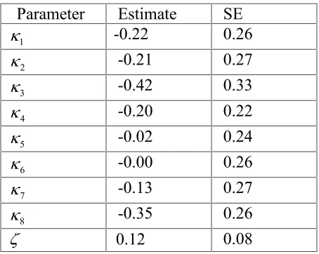
0.1089, so that systematically increasing the daily transportable cod eggs by 1 unit leads to about 11% increase in local cod abundance in Southern Norway, on the average. Table 3.1 reports the rest of the parameter estimates. In particular, all intercept terms are non-significant, and so is the coefficient estimate of  .

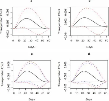
Figure 3. The plot of b ψjversus day j for the North Sea cod – the central solid line in each graph;

day 0 corresponds to March 1. The confidence bands are shown for a) frequentist (dashed line is 95%), b) Bayesian (dashed line is 95%), c) nonparametric bootstrap (dashed line is 95%, dotted-dashed line is 90%), and d) parametric bootstrap (dotted-dashed line is 95%, dotted-dotted-dashed line is 90%) methods.

Model checking procedures were done on our data by examining the residuals. To save space, diagnostics figures are not shown, but we note that the residual against the fitted value plot suggests no residual nonlinearity and that the residuals have constant variance. The time plot of the residuals (not shown) displays no temporal patterns. The normal Q-Q plot of the residuals appears mostly straight. These model diagnostics suggest that the model assumptions seem reasonable.

constant over 2-week periods (Stenseth et al. 2006). However, our new method allows for much more refined conclusions of great importance to the field of marine ecology.

Table 1: Estimates of model parameters for the Skagerrak cod.

Parameter Estimate SE

1

 -0.22 0.26

2

 -0.21 0.27

3

 -0.42 0.33

4

 -0.20 0.22

5

 -0.02 0.24

6

 -0.00 0.26

7

 -0.13 0.27

8

 -0.35 0.26

 _0.12 0.08

5. Simulation

We investigate the empirical performance of the proposed method by simulations. We will study two matters: the number of significant modes detected and the error involved in the estimates. The simulation model is motivated by the cod example:

= T ; = 1, , ,

t   bt t tb  t t T

Y c e  (5.1)

where Y_t is the response vector of dimension S1,  ,  , and are parameters, and b_t

and ct are covariates, where the dimension of the vectors and ct is D1 for both. The

error vector e_t has a multivariate normal distribution with mean zero and variance-covariance matrix 2

eP

 , where P is a correlation matrix.

In the examples below, T = 50, S = 3, D= 61, _ = [1,0, 1]_ T_{, and  = 1. The value of} t

b is determined by taking a random number from a normal distribution with mean zero and standard deviation one, while the value of ct are determined by creating a vector of

sixty-one random numbers from a normal distribution with zero mean and unit variance. There will be two levels of the error standard deviation: either 0.05 or 0.1. We will use a correlation matrix that is compound symmetric, meaning that

1

= 1

1

P

 

 

 

 

 

 

 

 

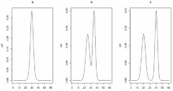
where there are four levels of _: 0.2_{, 0.2, 0.5, and 0.9. The} _j equals the probability density function at j of an equal mixture of two normal distributions, namely

(30 ,9)

 has two modes that are separated by either 20 units, 10 units, or 0 units (thus making one mode). Each case was simulated 1,000 times. The plots of the three different sets of

 's used can be found in Figure 4.

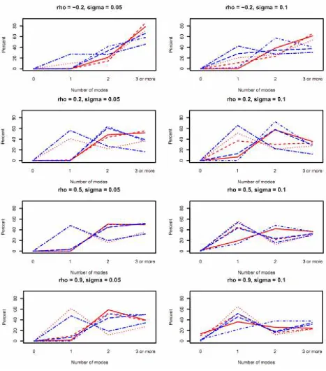
Simulation results are summarized in Figure 5. Recall the simulation was used to study two aspects of the problem: the number of significant modes detected (based on 95% confidence band) and the error involved in the estimates. Recent works have made a comparison between the Bayesian and frequentist approaches for the case of curves with continuous arguments (Wood 2006b), which we also do here with the confidence bands computed via either the frequentist approach, i.e. using Formula (3.1), or the Bayesian approach. In regard to the first aspect, Figure 5 shows that the simulation catches unimodality and multimodality fairly well when the correlation is high and the error variance is low. (Note that we count the number of modes only for the j's that are

significantly different from zero, hence there could be no mode in the curve if none of the

j

 's are significant.) The Bayesian confidence bands tend to catch unimodality and bimodality better than the frequentist confidence bands when the correlation is closer to zero. It seems that the two methods give similar results with a correlation around 0.5. The frequentist confidence bands tend to catch unimodality and bimodality better than the Bayesian confidence bands when the correlation is around 0.9. As far as the second aspect, the mean absolute deviation and mean deviation (unreported) were small as compared to the maximum value of the  's being estimated. Their standard deviations were small as well and depended proportionately on the error variance.

Figure 4. Plots of ψjversus j for the simulation model; ψjis the probability density function of the

Figure 5.Percents of 0, 1, 2, 3 or more modes detected. Red dotted lines: frequentist, ∆ = 0; red dashed lines: frequentist, ∆ = 5; red solid lines: frequentist, ∆ = 10; blue twodash lines: Bayesian, ∆ = 0; blue longdash lines: Bayesian, ∆ = 5; blue dashdot lines: Bayesian, ∆ = 10.

6. Conclusion

refined conclusion within the field of marine ecology, particularly with reference to how different populations of a marine fish species are interlinked through larvae inflow. As such, our results are of direct relevance for studies on the ecological effects of climate change (see, e.g., Stenseth, Mysterud, Ottersen, Hurrell, Chan, and Lima (2002)).

There are a few interesting future research problems. First, it is of interest to work out the case of non-normal errors in greater details. Second, the common transfer function assumption is a strong one. A more flexible approach is to incorporate random-effects in the transfer function model.

Acknowledgements

We are grateful to Chong Gu for valuable suggestions. We thank Halvor Knutsen for assistance in making Figure 2. The empirical work referred to above was done in collaboration with colleagues at the Institute of Marine Research, Flødevigen IMR, Lysekil and Tjärnö Marine Biological Laboratory; that work was funded by the Norwegian Research Council, the Swedish Council for the Environment and the Nordic Council of Ministers supported this work. Work reported in this paper was supported financially by the Norwegian Research Council, the University of Oslo and the National Science Foundation (NSF DMS-0934617).

References

1. Almon, S. (1965), “The distributed lag between capital appropriations and expenditures,” Econometrica, 33, 178 – 196.

2. Box, G., Jenkins, G., and Reinsel, G. (1994), Time Series Analysis, Forecasting and Control, San Fransisco, California, USA: Pearson Education.

3. Chan, K.-S., Stenseth, N. C., Kittilsen, M., Gjosæter, J., Lekve, K., Smith, T., Tveite, S., and Danielssen, D. (2003a), “Assessing the effectiveness of releasing cod larvae for stock improvement: using long-term beach-seine monitoring data to resolve a century-long controversy,” Ecological Applications, 13, 3 – 22.

4. Chan, K.-S., Stenseth, N. C., Lekve, K., and Gjosæter, J. (2003b) “Modeling pulse disturbance impact on cod population dynamics; the 1988 algae bloom of Skagerrak, Norway,” Ecological Monographs, 73, 151 – 171.

5. Corradi, C. (1977), “Smooth distributed lag estimators and smoothing spline functions in Hilbert space,” Journal of Econometrics, 5, 211 – 219.

6. Efron, B. and Tibshirani, R. (1998), An Introduction to the Bootstrap, Boca Raton: Chapman & Hall/CRC.

7. Green, P. and Silverman, B. (1994), Nonparametric Regression and Generalized Linear Models, London, England: Chapman and Hall.

8. Gu, C. (2002), Smoothing Spline ANOVA Models, New York, USA: Springer-Verlag.

10. Han, C. and Gu, C. (2008), “Optimal smoothing with correlated data,” Sankhyā: The Indian Journal of Statistics, 70-A, 38–72.

11. Kitagawa, G. and Gersch, W. (1996), Smoothness Priors Analysis of Time Series, New York, USA: Springer-Verlag.

12. Knutsen, H., André, C., Jorde, P., Skogen, M., Thuroczy, E., and Stenseth, N. C. (2004), “Transport of north sea cod larva into the Skagerrak coastal populations,” Proceedings of the Royal Society of London, B, 271, 1337–1344.

13. Reinsel, G. and Velu, P. (1998), Multivariate reduced-rank regression: theory and applications, New York: Springer-Verlag.

14. Shiller, R. (1973), “A distributed lag estimator derived from smoothness priors,” Econometrica, 41, 775 – 788.

15. Stenseth, N., Jorde, P., Chan, K., Hansen, E., Knutsen, H., André, C., Skogen, M., and Lekve, K. (2006), “Ecological and genetic impact of Atlantic cod larval drift in the Skagerrak,” Proceedings of the Royal Society of London, B, 273, 1085–1092.

16. Stenseth, N. C., Mysterud, A., Ottersen, G., Hurrell, J., Chan, K.-S., and Lima, M. (2002), “Ecological effects of climate fluctuations,” Science, 297, 1292–1296. 17. Wahba, G. (1990), “Spline models for observational data,” Philadelphia: SIAM. 18. Wood, S. (2000), “Modelling and smoothing parameter estimation with multiple

quadratic penalties,” Journal of Royal Statistical Society, B62, 413–428.

19. Wood, S. (2004), “Stable and efficient multiple smoothing parameter estimation for generalized additive models,” Journal of the American Statistical Association, 99, 673–686.

20. Wood, S. (2006a), Generalized Additive Models: An Introduction with R, Chapman & Hall/ CRC.

21. Wood, S. (2006b), “On confidence intervals for generalized additive models based on penalized regression splines,” Australian & New Zealand Journal of Statistics, 48, 445–464.