Parameterization for subgrid-scale motion of ice-shelf calving fronts
T. Albrecht1,2, M. Martin1,2, M. Haseloff1,3, R. Winkelmann1,2, and A. Levermann1,2
1Earth System Analysis, Potsdam Institute for Climate Impact Research, Potsdam, Germany 2Institute of Physics, University of Potsdam, Potsdam, Germany
3Earth and Ocean Science, University of British Columbia, Vancouver, Canada
Received: 15 July 2010 – Published in The Cryosphere Discuss.: 27 August 2010
Revised: 15 December 2010 – Accepted: 29 December 2010 – Published: 19 January 2011
Abstract. A parameterization for the motion of ice-shelf fronts on a Cartesian grid in finite-difference land-ice mod-els is presented. The scheme prevents artificial thinning of the ice shelf at its edge, which occurs due to the finite reso-lution of the model. The intuitive numerical implementation diminishes numerical dispersion at the ice front and enables the application of physical boundary conditions to improve the calculation of stress and velocity fields throughout the ice-sheet-shelf system. Numerical properties of this subgrid modification are assessed in the Potsdam Parallel Ice Sheet Model (PISM-PIK) for different geometries in one and two horizontal dimensions and are verified against an analytical solution in a flow-line setup.
1 Introduction
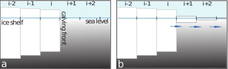
Ice shelf fronts are predominantly observed to have an almost vertical cliff-like shape with a typical ice thickness of a few hundred meters (idealized sketch in Fig. 1a). Bending of this ice wall imposes strong tensile and shear stresses close to the terminus and promotes crevassing (Reeh, 1968; Scambos et al., 2009). Calving icebergs are cut off from the shelf along intersecting crevasses (Kenneally and Hughes, 2006) and are swept away onto the open ocean where they melt.
As a precondition for the computational treatment of calv-ing processes and for imposcalv-ing the correct boundary condi-tions and thereby properly computing the stress field within the shelf, we focus here on the subgrid-scale motion of the ice front on a fixed rectangular grid. One challenge arises through the finite resolution when the ice front advances sea-ward. Without special treatment the ice flux into a newly
Correspondence to: A. Levermann ([email protected])
occupied grid cell is spread out over the entire horizontal do-main of the grid cell (Fig. 1b). Thus, the finite-difference ice-transport scheme (here first-order upwind) can produce grid cells of only a few meters ice thickness (or even less). In numerical models these cells are considered as floating ice-shelf grid cells whose front propagates one grid cell ahead at each time step. This is generally faster than the motion of the actual moving ice-shelf margin and has no proper physi-cal basis. The model hence produces a situation in which the ice front has no sharp vertical profile as it should have but an unphysical extension in the direction of the open ocean. In such a situation also the corresponding ice-thickness gradient which drives the ice flow is unrealistic. The dispersion effect depends mainly on the time step and spatial discretization length. It should be distinguished from the numerical diffu-sion of an upwind mass-transport scheme, which is often ap-plied in finite difference models and takes the form of an ad-ditional diffusion term due to the asymmetry of the scheme.
a
i-2 i-1 i i+1 i+2
b
i-2 i-1 i i+1 i+2
ca
lv
in
g f
ro
nt
sea level
ice shelf
Fig. 1. (a)
Schematic of a discretized ice shelf is shown in lateral view with decreasing ice thickness in
positive i-direction. The local calving front is located at the interface between the last shelf grid cell
[
i
]
and the adjacent open ocean cell
[
i
+1]
.
(b)
In every time step a volume increment is calculated for each
grid cell according to the scheme approximating Eq. (1). Thus, in every time step, the marginal cliff
moves one grid cell further into the open ocean and may thin out relatively fast.
19
Fig. 1. (a) Schematic of a discretized ice shelf is shown in lateral view with decreasing ice thickness in positive i-direction. The local calving front is located at the interface between the last shelf grid cell[i]and the adjacent open ocean cell[i+1]. (b) In every time step a volume increment is calculated for each grid cell according to the scheme approximating Eq. (1). Thus, in every time step, the marginal cliff moves one grid cell further into the open ocean and may thin out relatively fast.
The paper is organized in three main parts. In Sect. 2 the features of PISM-PIK that are directly relevant for the calv-ing front are briefly summarized. Section 3 introduces the proposed subgrid-parameterization of ice-front motion in the flow-line case and its generalization to flow in two horizontal dimensions. In Sect. 4 the parameterization is tested in sim-ulations with PISM-PIK for a flow-line setup as well as for the Larsen and Ross Ice Shelves. We conclude in Sect. 5.
2 Model description
The parameterization for subgrid-scale ice-front motion, in-troduced in Sect. 3, is applied in the Potsdam Parallel Ice Sheet Model, PISM-PIK, which is based on the thermo-mechanically coupled open-source Parallel Ice Sheet Model (PISM stable 0.2 by Bueler et al., 2008). Within the model, the stress balance for a floating ice shelf with negligible basal friction is computed according to the Shallow Shelf Ap-proximation (SSA, Morland, 1987; MacAyeal, 1989; Weis et al., 1999) on a fixed rectangular grid. Solving the stress-balance equations in SSA with appropriate boundary condi-tions yields vertically integrated velocities, which are used for horizontal ice-transport. A full description of the model is provided by Winkelmann et al. (2010) and its performance in a setup of the Antarctic ice sheet under present-day bound-ary conditions is discussed by Martin et al. (2010). Here we summarize some aspects relevant for the parameterization.
The mass-transport scheme is particularly important for the ice-front motion. It approximates the ice-flux equation. In order to illustrate the general idea we restrict ourselves to the one-dimensional (flow-line) case
∂V ∂t =a
∂H ∂t = −a
∂(vxH )
∂x , (1)
withV,H,vx anda being ice volume, thickness, velocity and area of a grid cell (variables summarized in Table 1). For simplicity we ignore surface and bottom mass balance.
In the vicinity of a discontinuity like a propagating ice-shelf front the appropriate numerical discretization is an upwind transport scheme. PISM base code (Bueler and Brown, 2009) uses a combination of an upwind and a centered scheme in the SSA region which does not conserve the total numerical ice mass. In PISM-PIK we introduce a first-order upwind scheme on a staggered grid which is based on the finite vol-ume method (as generally discussed in Morton and Mayers, 2005). At the ice-front boundary the scheme has to be ad-justed since there are no ice velocities on the open ocean. In accordance with the applied conservative upwind scheme we get for the flux through the boundary (with terminal ice thicknessHcand terminal velocityvc) into the adjacent grid cell on the seaward side of the ice-shelf front
1H=vcHc1t /1x. (2)
The Courant-Friedrichs-Lewy criterion (CFL, Courant et al., 1928, 1967) guarantees numerical stability, i.e., the volume increment advected to the ocean grid cell is always smaller than the ice volume of the last shelf cell,
|1V| =aHc
|v
c|1t
1x
≤aHc. (3)
This will play a role in the discussion of the treatment of residual ice volume in Sect. 3.
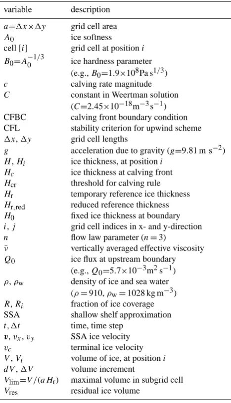
variable description
a=1x×1y grid cell area A0 ice softness cell[i] grid cell at positioni B0=A
−1/3
0 ice hardness parameter (e.g.,B0=1.9×10⁸Pa s1/3) c calving rate magnitude C constant in Weertman solution
(C=2.45×10⁻¹⁸m−3s−1) CFBC calving front boundary condition CFL stability criterion for upwind scheme 1x,1y grid cell lengths
g acceleration due to gravity (g=9.81 m s−2) H,Hi ice thickness, at positioni
Hc ice thickness at calving front Hcr threshold for calving rule Hr temporary reference ice thickness Hr,red reduced reference thickness H0 fixed ice thickness at boundary i,j grid cell indices in x- and y-direction n flow law parameter (n=3)
¯
ν vertically averaged effective viscosity Q0 ice flux at upstream boundary
(e.g.,Q0=5.7×10⁻³m2s−1) ρ,ρw density of ice and sea water
(ρ=910,ρw=1028 kg m−3) R,Ri fraction of ice coverage SSA shallow shelf approximation t,1t time, time step
v,vx,vy SSA ice velocity vc terminal ice velocity V,Vi volume of ice, at positioni dV,1V volume increment
Vlim=V /(a Hr) maximal volume in subgrid cell Vres residual ice volume
of the positivex-axis the physical stress balance for the two coordinate directions reads
(ν H¯ c)|j
i+12
2∂vx
∂x + ∂vy
∂y j
i+12
= ρg 2
1− ρ
ρw
Hc2|ji,
(ν H¯ c)| j
i+12
∂v
x ∂y +
∂vy ∂x
j
i+12
=0. (4)
At these positions the hydrostatic pressure term of the bound-ary condition (right-hand side of the equations) substitutes the velocity gradients used in the SSA equations (withν¯ as vertically averaged effective viscosity). In PISM-PIK we ap-ply the dynamic boundary condition for each shelf grid cell facing the ocean to at least one side (for details see Winkel-mann et al., 2010), Our subgrid parameterization guarantees a steep calving front and hence yields the correct stress bal-ance.
ization we apply a simple calving condition that has been used in a number of previous model studies (Ritz et al., 2001; Peyaud et al., 2007; Paterson, 1994). It is based on the fact that observed ice thicknesses at calving fronts in Antarctica vary mostly between 150 and 250 m. We thus eliminate ice in any grid cell that (1) is located at the calving front and (2) has ice thickness less than a critical thresholdHcr. The
results are qualitatively independent of the specific choice of Hcrfor which we use a value of 250 m throughout the paper.
3 Parameterization
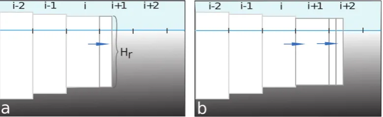
In this section we describe the subgrid parameterization of ice-front motion for both the flow-line case (one horizontal dimension) and generalize to ice flux in two horizontal di-mensions. For the discretized ice-shelf model with clear-cut terminal cliff at grid cell[i](as illustrated in Fig. 1a) the dis-cretized flux equation Eq. (2) yields an ice-volume increment to be added to the adjacent ocean grid cell[i+1]with hori-zontal areaa. The corresponding volume increment1Vi+1
is, without our scheme, associated with a thin ice layer of thickness1Hi+1=1Vi+1/a covering the whole surface of
the grid cell. In our implementation a volume increment is associated with a slab ice block adjacent to the cliff (Fig. 2a). To that end, we define a field that has the valueR=1 on shelf grid cells andR=0 on ice-free ocean grid cells. Scalar values 0<R<1 in grid cells at the interface between shelf and ice-free ocean are associated with the ratio of ice covered hori-zontal area in a grid cell with a defined reference ice thick-nessHrto the total grid-cell areaa, which is calculated as
R= V aHr
, (5)
whereV is the current ice volume within the partially-filled grid cell[i+1]. Thus, the slab ice block of ice thickness Hrcovers an areaa R of the grid cell. In the flow-line case
we choose this reference value to be equal to the ice thick-nessHr≡Hc of the adjacent shelf cell of the previous time step. In a dynamic simulation a positive ice flux through the boundary yields a new volume increment at each time step that is added to the boundary grid cell[i+1]. Consequently, the area in the grid cell covered with ice and hence the ratio Rincreases. An increasingR is interpreted as an advancing front within a grid cell, i.e., on subgrid scale.
When the ice volume in grid cell[i+1]exceeds the thresh-old Vlim=aHr, this ice-shelf grid cell is considered to be
full withR=1. In the next time step the adjacent grid cell [i+2] can start growing in ice volume (Fig. 2b). During this forward propagation of the front boundary the terminal ice thicknessHcmight change. Hence, the ratioRchanges sinceHris updated each time step even if there is no ice flux
a
i-2 i-1 i i+1 i+2
b
i-2 i-1 i i+1 i+2
Hr
Fig. 2.
Lateral view of discretized ice shelf with subgrid-scale parameterization.
(a)
The volume
incre-ment in grid cell
[
i
+1]
is associated with a slab of ice of the same ice thickness as the adjacent full shelf
grid cell
[
i
]
.
(b)
When the grid cell
[
i
+1]
at the calving front is full of ice according to the associated
reference thickness, the next following cell
[
i
+2]
can gain in ice volume.
20
Fig. 2. Lateral view of discretized ice shelf with subgrid-scale parameterization. (a) The volume increment in grid cell[i+1]is associated with a slab of ice of the same ice thickness as the adjacent full shelf grid cell[i]. (b) When the grid cell[i+1]at the calving front is full of ice according to the associated reference thickness, the next following cell[i+2]can gain in ice volume.
Retreat of the ice-shelf front in response to a continuous calving rate (e.g., Benn, 2007, Eq. 1) can be treated in a sim-ilar fashion as the ice advance. In the following experiments we use a simple calving condition as prescribed in Sect. 2. A generalization to other calving laws is straight forward. In such a situation, a partially filled grid cell is drained with a negative fluxQ−= −c Hr, where c is the magnitude of the calving rate. If the grid cell is empty withVi+1≤0,
fur-ther ice loss acts onto the adjacent ice-shelf grid cell with Ri=1+Vi+1/(a Hc)≤1. Analogous to the CFL-limited nu-merical propagation speed of the front also the retreat is thereby restricted to at most one grid cell per time step for the simple calving rule as well as for more sophisticated calving-rate parameterizations. Negative ice volumes are set to zero after this procedure.
The generalization of Eq. (1) to two-dimensional horizon-tal ice volume flux is simply
∂V ∂t =a
∂H
∂t = −adiv(vH ), (6)
with a generalized CFL-criterion as in the PISM base code 1tadapt=min
i,j
|u
i,j|
1x + |vi,j|
1y + ε 1x+1y
−1
, (7)
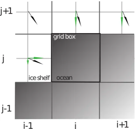
whereεis a small factor to avoid division by zero. As an ex-ample, grid cell[i,j]in Fig. 3 borders two ice-shelf cells with velocity components directed to this grid cell on the ice-free ocean. Here, the reference ice thicknessHr is the average
of the ice thicknesses of those two neighboring shelf cells (or better a flux-weighted average). The volume flux through the two boundaries together with the volume of the previous time step adds up to the new volumeVi,j. Herewith the ratio Ri,j of ice-covered area in this grid cell is evaluated.
When a subgrid ice front advances and a grid cell at the boundary is considered to become full (R=1) according to the reference thicknessHrit is possible that some residual
ice volume remains unaccounted for
Vres=V−Vlim. (8)
A convenient way to treat this remaining volume is to sim-ply omit it (variant 1). Obviously this has the disadvantage of an artificial ice loss but the advantage that it does not in-terfere with the ice-shelf dynamics upstream of the moving ice front becauseHcis properly represented. Hence, the im-posed CFBC, which is evaluated at the ice-shelf front and de-pends sensitively on the boundary ice thicknessHc(Eq. 4), enables the accurate computation of velocities according to the SSA throughout the ice shelf.
In order to conserve numerical ice mass and to still keep the numerical treatment as simple as possible, the residual ice mass can alternatively be equally redistributed to the neigh-boring grid cells on the ice-free ocean (variant 2). For these adjacent cellsHr must be determined. Using adaptive time
steps according to the CFL-stability criterion (Eq. 3) guar-antees that the size of the volume increments1V advected to the next ocean grid cell is limited. In the model of an unconfined ice shelf (e.g., flow-line case) a special problem occurs because the largest velocities are typically found at the evolving front. There, the advection of the ice-thickness discontinuity as in Eq. (2) has maximum propagation speed of one grid length 1x per time step 1t. Hence, we have max(Vres)=a Hc, which is redistributed to the adjacent grid cell[i+2]. If we chooseHr=Hcthis cell at the interface be-tween ice shelf and ice-free ocean is completely filled within one time step (Ri+2=1), and the ice shelf evolves with an ice
wall at the front that does not decrease in ice thickness, which has a strong impact on the dynamics throughout the ice shelf. In order to avoid this problem for variant 2 we reduce the ref-erence thickness toHr,redand make a linear guess according
to the analytical solution (Eq. 11), which is described in the next section. The expected slope at the front depends mainly on the power law of the marginal ice thicknessHcand typical constant ice parameterCand boundary valuesQ0
Hr,red≡Hr+ ∂H
∂x
c
1x=Hr− C
Q0
j
j-1
i
i+1
i-1
ocean
ice shelf
grid box
Fig. 3. A bird’s eye view of the ice shelf calving front approximated by a rectangular mesh grid. Gray shaded area denotes ice-free ocean, the ice shelf area is white with exemplary velocity vectors defined on the regular grid. Velocity components directed to the open ocean are shown in green.
21
Fig. 3. A bird’s eye view of the ice shelf calving front approxi-mated by a rectangular mesh grid. Gray shaded area denotes ice-free ocean, the ice shelf area is white with exemplary velocity vec-tors defined on the regular grid. Velocity components directed to the open ocean are shown in green.
This solves the problem of the unrealistic thick ice wall at the front for adaptive time steps. Note that even an inaccurate guess for the reference ice thickness jeopardizes neither mass conservation nor the basic idea of the parameterization.
4 Application in numerical simulations
As mentioned before, the membrane-stress balance in SSA is a non-local boundary-value problem and its over-all solution is controlled by the boundary conditions. Thus the introduc-tion of a numerical method that alters the boundaries requires verification against an analytical solution. It is a robust fea-ture of unconfined ice shelves that the thinning rate becomes smaller with increasing distance from the grounding line. In the model the position of the calving front of a certain ice thickness (e.g., 250 m) is sensitive to this ice thickness itself and hence small variations in ice transport have a noticeable effect. This makes the flow-line setup with applied calving rule to be a strong sensitivity test of the proposed parameter-ization.
For a first assessment we apply a simple ice-shelf setup, where the flow is one-dimensional in the sense that all quan-tities perpendicular to the flow line are constant and only the unidirectional spreading of ice is considered. We apply peri-odic boundary conditions at the lateral boundaries, which is associated with an infinitely broad unconfined ice shelf. At the upstream boundary, ice thickness and velocity are pre-scribed to 600 m and 300 m/yr. The bathymetry can be
cho-account here. There is no thermocoupling since a constant ice hardness ofB0=1.9×10⁸Pa s1/3according to MacAyeal
et al. (1996) is used.
The model solution is compared with the following analytical solution of the flow-line case. We choose the x-axis as the direction of the main ice flow with constant ice inflowQ0=vx,0H0and with vanishing transversal
com-ponents. In the flow-line case the stress equilibrium equa-tions in SSA simplify considerably. Since ice is treated as a non-linearly viscous, isotropic fluid with a constitutive rela-tion of Arrhenius-Glen-Nye form (Paterson, 1994) the equa-tions can be integrated and rearranged with constant hardness B0=A
−1/n
0 and flow-law exponentn=3. The solution for the
spreading rate was first found by Weertman (1957) to be ∂vx
∂x =
ρg 4B0
1− ρ
ρw
H
3
=C H3. (10)
Inserting this into the ice-thickness Eq. (1), we obtain af-ter integration the ice thickness and velocity profiles for the steady state (Van der Veen, 1999),
H (x)= 4C Q0
x+ 1 H04
!−1/4
, (11)
vx(x)= Q0
H (x)=Q0 4C Q0
x+ 1 H04
!1/4
. (12)
There is no ice-shelf front considered in the analytical steady state, since lim
x→∞H (x)=0. But when appropriate boundary conditions are applied we can assume that the modeled tran-sient profile is congruent to the analytical profile up to the advancing front at position xc. This theoretical position of the free boundary at timet can be derived from integration ofQ0t=
Rxc
0 H (x
0)dx0, which yields
xc(t )= Q0
4C
3C t+
1 H03
!4/3
− 1 H04
. (13)
0 150 300 450 600
ice thickness (m) (a)
no CFBC with CFBC
0 100 200 300 400
0 250 500 750 1000
ice velocity (m/yr)
distance (km)
(b)
Fig. 4. Profiles of ice thickness (top) and velocity (bottom) in flow-line case in lateral view after evolution time 1000 yr. Fixed Dirich-let boundary on the left and calving front on the right hand side of the computational domain. Blue: the result with applied CFBC al-ready in steady state. Green: with shelf-extension scheme and still advancing. Black dashed is the expected profile from analytical so-lution in steady state when cut off at 250 m ice thickness. In both cases a resolution of 101×5 km, adaptive time stepping and vari-ant 1 of residual mass treatment are used.
When using the standard extension scheme with vanish-ing velocities at the boundary of the computational domain, the experiment shows that the velocity profile underestimates the analytical solution by more than 100 m/yr in the outer re-gions of the ice shelf (>100 km). Consequently, with con-stant ice flux across the profile, the ice thickness profile can be expected to be too thick, here about 60 m at the termi-nus. When applying the CFBC, however, the profile of the velocity is steeper and on average only 9 m/yr less than the the exact solution profile. Thus, calving front ice thickness of 250 m is reached at a position 10 km close to the position expected from the analytical solution (Fig. 4a, dashed). Ice-shelf velocities are calculated independently of velocities on the ice-free ocean, which enhances the performance.
The CFBC gives best results when the calving front has a rectangular shape (in side view, as in Fig. 2). This shape is guaranteed with the examined subgrid treatment at the calv-ing front. Without the subgrid parameterization though, we observe a disperion of the steep ice front with grid cells of very thin ice at the front (Fig. 1b). Hence, the CFBC is applied at a false position for a false terminal ice thickness Hc. Accordingly, the velocity calculation gives false results throughout the whole ice shelf.
0 150 300 450 600
ice thickness (m) (a)
51 x 10km
101 x 5km
201 x 2.5km
0 100 200 300 400
0 250 500 750 1000
ice velocity (m/yr)
distance (km)
(b)
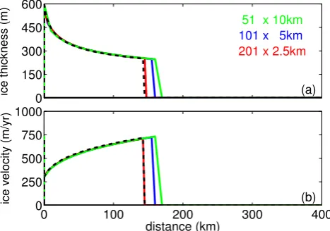
Fig. 5. Steady-state flow-line ice thickness and velocity profiles in lateral view calculated with different resolution but constant size of computational domain. Calving front position (145 km) and ter-minal velocity (720 m/yr) as expected from the analytical solution with constant ice hardness for 250 m terminal ice thickness are shown as black dashed line. Adaptive time steps and variant 1 of residual ice treatment are used.
0 150 300 450
ice thickness (m) (a)
0 100 200 300 400
0 250 500 750 1000
ice velocity (m/yr)
distance (km)
(b)
0 150 300 450 600
ice thickness (m) (c)
variant 1
0 100 200 300 400
0 250 500 750 1000
ice velocity (m/yr)
distance (km)
(d)
0 150 300 450 600
ice thickness (m) (e) variant 2
0 100 200 300 400
0 250 500 750 1000
ice velocity (m/yr)
distance (km)
(f)
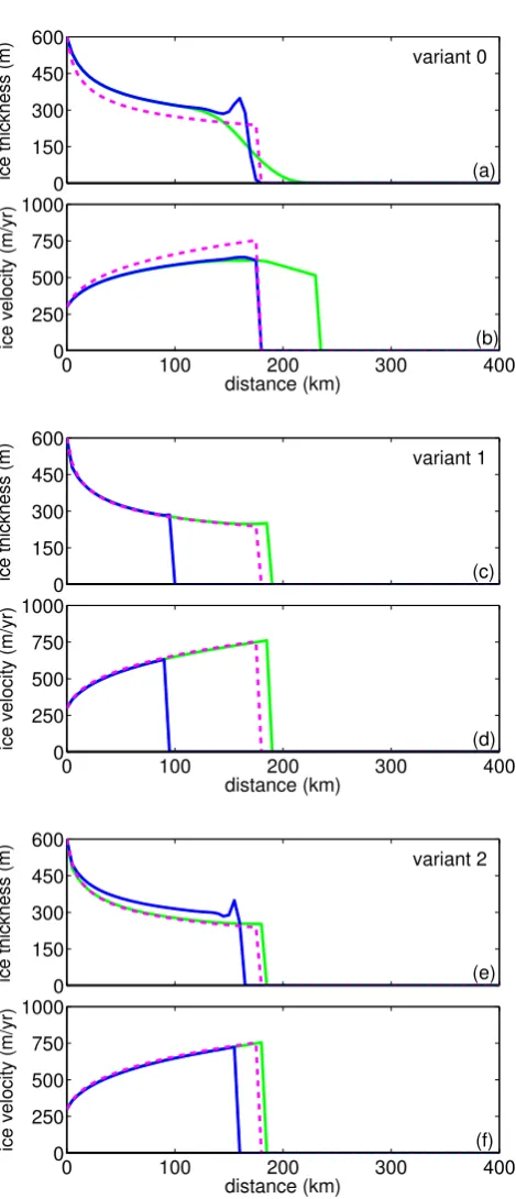
Fig. 6. Transient flow-line ice thickness and velocity profiles in lateral view after 300 yr of time evolution, calculated using three different variants of residual mass treatment. The model result with adaptive time stepping is shown in blue, i.e.,1t≈6–10 yr. The re-sult with fixed short time step1t=1 yr is plotted in green. Magenta dashed is the analytical profile after evolution timet=300 yr. A res-olution of 101×5 km is used. CFBC and subgrid parameterization are not applied for the control case variant 0.
at the boundary, different effects of the two variants of treat-ment of residual ice volumes are revealed. For comparison a simulation is shown where none of the two described variants of subgrid calving front treatment is used (denoted as “vari-ant 0”), so basically the PISM extension scheme with vanish-ing velocities at the boundary of the computational domain. In this case, the propagating calving front suffers from strong numerical dispersion (ice thickness declines by 250 m over a distance of 80 km) especially for small time steps about 10 times shorter than adaptive time steps (Fig. 6a, green, 1t=1 yr). Thus, grid cells of very thin ice occur in the ter-minus region and the related velocities decrease in flow-line direction (Fig. 6b, green) influenced by velocity calculation in the region of the ice-free ocean and the by the shape of the dispersed front. For adaptive time steps though (Fig. 6a, blue) the front is much steeper, but a rather small numeri-cal effect at the front is observed, so numeri-called “wiggles”, which will be discussed later. Upstream of the front, in both tran-sient cases the computed ice thickness profiles overestimate the analytical solution, which can be expressed in terms of the coefficient of determination, which is for adaptive time stepsr2=0.81 and for short time steps slightly better (value 1 means perfect match). Consequently, with application of calving at a certain ice thickness, a steady-state front posi-tion far beyond the analytical one can be anticipated. This is analogous to the first experiment result (Fig. 4) where the shelf-extension scheme was applied.
If we use the subgrid parameterization and cut off the oc-curring residual ice volumes (variant 1) we get accurately shaped profiles according to the analytical solution both in the transient phase (Fig. 6c, d) and in steady state (Fig. 5) with a coefficient of determination of r2>0.97 close to 1. The big advantage of this procedure is the rectangular shape of the calving front without any disturbing wiggles through-out the whole transient phase. This leads to a proper appli-cation of the CFBC and accurate velocity profiles (Fig. 6d). Variant 1 produces a certain mass loss, which can be easily reported and discussed (it is not caused by the actual trans-port scheme). The mass loss is negligible for small time steps (green) but it is quite large in a shelf propagating with max-imal time steps according to the CFL-criterion (blue), which can be seen in the deviation of the front position in relation to the analytical front.
N E
S
W
Fig. 7. Realistic steady-state model simulation of Larsen A and B Ice shelf (light gray) with grounded parts (dark gray) and the ice-free ocean (white). Values ofRat the propagating ice shelf front are colored.
25
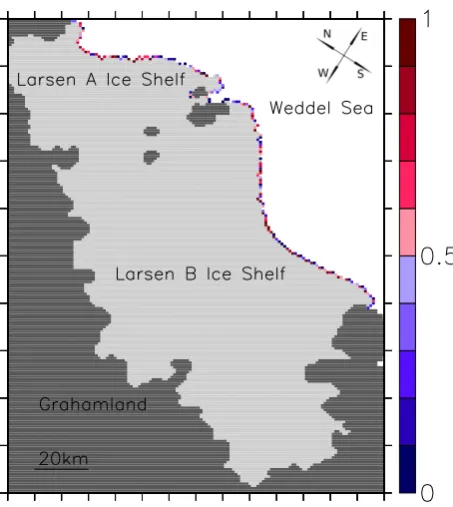
Fig. 7. Snapshot of a realistic steady state model simulation of Larsen A and B Ice shelf (light gray) with grounded parts (dark gray) and the ice-free ocean (white). Values ofRat the propagating ice shelf front are colored.
the CFBC evaluated at the last shelf grid cell leads to under-estimated velocity values along the ice shelf (Fig. 6f, blue), which gives a smallerr2=0.84. Hence, the ice shelf is on average 37 m too thick and the front lags behind the analyti-cally calculated front position (magenta dashed).
The subgrid-parameterization of ice-front motion with both variants of residual mass treatment is designed to be applied in two-dimensional and realistic setups as for Larsen A and B Ice Shelf as shown in Fig. 7 and for the Ross Ice Shelf in Fig. 8. Along the smooth ice front theR-field has values of 0≤R<1, while the ice shelf with valuesR=1 is shaded in light gray and grounded areas in dark gray. The figures show a steady state snapshot with applied continuous physical calving rate, but details are discussed elsewhere (Levermann et al., 2011).
In a two-dimensional realistic setup of a confined ice shelf or even in a setup of the Antarctic ice sheet with sev-eral ice shelves attached the adaptive time steps are deter-mined according to the maximal velocity magnitude of the whole computational domain (Eq. 7). The generalized CFL-criterion is used to limit the amount of residual ice mass, which is redistributed equally to the neighbor grid cells in an unphysical way with regard to the physical flow across the boundary. We could apply a more rigorous criterion, but simulations in realistic setups confirm that the error is small. The maximal flux through the boundary for a certain
adap-N E
S W
Fig. 8.Realistic steady-state model simulation of Ross Ice shelf (light gray) with grounded parts (dark gray) and the ice-free ocean (white). Values ofRat the propagating ice shelf front are colored.
26
Fig. 8. Snapshot of a realistic steady state model simulation of Ross Ice shelf (light gray) with grounded parts (dark gray) and the ice-free ocean (white). Values ofRat the propagating ice shelf front are colored.
tive time step occurs for a single pair of cells, which is lo-cated probably at the ice front with distance from confine-ments, whereas along the rest of the ice-shelf front velocities are lower than the maximal value. Numerical damping is rel-atively efficient in most front regions as well as in the inner parts of the ice shelf. Hence, transient phenomena like wig-gles at the front are rarely observed.
5 Discussion and conclusions
In this paper we presented a numerical method that enables the subgrid motion of ice-shelf fronts in a finite-difference model. This prevents the steep margin from being numer-ically dispersed and allows for a proper application of the Neumann boundary condition for the approximated stress-balance calculations. Flow-line simulations with the Pots-dam Parallel Ice Sheet Model (PISM-PIK) for different res-olution have been compared with the exact analytical solu-tions. The modification of the transport scheme at the ice-front boundary, which implicates a redistribution of residual ice volumes at this moving front has been assessed and dis-cussed. The proposed procedure opens the way to an ap-propriate determination and application of calving rates in realistic models of combined ice-sheet/ice-shelf dynamics.
straight (not discussed in this paper). An additional bene-fit in using the implemented CFBC is that velocity calcula-tion is independent of informacalcula-tion outside of the ice-shelf boundaries. Thus, velocities on the ice-free ocean can be ig-nored, which simplifies the calculation of SSA-velocities and reduces computational cost. Very well approximated steady-state ice thickness and velocity profiles with a coefficient of determination ofr2>0.99 are observed for all of the three tested resolution. The steady-state front position converges to the analytical solution for resolution refinement. In sim-ulations of the Antarctic ice sheet (e.g., Martin et al., 2010), coarse resolution of about 20 km grid length or more are used and marginally overestimated mass fluxes can be expected here in the ice-stream and shelf region.
The subgrid parameterization of ice-shelf-front motion implicates the handling of residual ice-volume increments that arise from the restriction R≤1 of the ice coverage ra-tio. We show in transient simulations that variant 1 yields very accurate flow-line profiles for both ice thickness and ve-locity, although the modeled front lags behind the analytical front due to the cut-off of residual ice volumes. We use this variant for the application of calving rates that depend sen-sitively on the velocity field in the vicinity of the front (e.g., Levermann et al., 2011). Thereby, the residual ice volumes are reported as additional mass loss, although they are not physically motivated. Note that in the flow line case with adaptive time stepping (Fig. 6c, blue) variant 1 can produce large mass losses. In a more realistic case, however, these mass losses are far smaller, comparable to the flow-line case of shorter time steps (as in Fig. 6c, green) since the residual ice volumes are generally much smaller and the cut-off oc-curs less often. The mass-conservative variant 2, however, yield accurate results and does not increase computational cost distinguishably since the CFL-criterion limits the size of the volume increments and the numerical redistribution of residual ice volumes to adjacent grid cells on the ocean is generally executed only once each time step.
Acknowledgements. T. Albrecht and M. Haseloff were funded by the German National Academic Foundation (Studienstiftung des deutschen Volkes), M. Martin and R. Winkelmann by the TIPI project of the WGL. We thank Ed Bueler and colleagues (University of Alaska, USA) for providing the sophisticated model base code and numerous advice, as well as Florian Ziemen (MPI Hamburg, Germany) for valuable discussions and helpful suggestions about numerical schemes. We are grateful to Xylar Asay-Davis and Dan Goldberg for reviewing the manuscript and suggesting a number of improvements.
Edited by: G. H. Gudmundsson
Bentley, C. R.: The Ross Ice shelf Geophysical and Glaciologi-cal Survey (RIGGS): Introduction and summary of measurments performed; Glaciological studies on the Ross Ice Shelf, Antarc-tica, 1973–1978, Antarct. Res. Ser., 42, 1–53, 1984.
Bueler, E. and Brown, J.: The shallow shelf approxima-tion as a sliding law in a thermomechanically coupled ice sheet model, J. Geophys. Res., 114, F03008, 21 pp., doi:10.1029/2008JF001179, 2009.
Bueler, E., Brown, J., Shemonski, N., and Khroulev, C.: PISM user’s manual: A Parallel Ice Sheet Model, http://www. pism-docs.org/, 2008.
Courant, R., Friedrichs, K., and Lewy, H.: ¨Uber die partiellen Dif-ferenzengleichungen der mathematischen Physik, Math. Ann., 100, 32–74, 1928.
Courant, R., Friedrichs, K., and Lewy, H.: On the partial difference equations of mathematical physics, IBM Journal, pp. 215–234, english translation of the 1928 German original, 1967.
Benn, D. I., Warren, C. R., and Mottram, R. H.: Calving processes and the dynamics of calving glaciers, Earth-Sci. Rev., 82, 143– 179, 2007.
Kenneally, J. P. and Hughes, T. J.: The calving constraints on in-ception Quternary ice sheets, Quatern. Int., 95–96, 43–53, 2002. Kenneally, J. P. and Hughes, T. J.: Calving giant icebergs: old
prin-ciples, new applications, Antarct. Sci., 18, 409–419, 2006. Levermann, A., Albrecht, T., Winkelmann, R., Martin, M. A.,
Haseloff, M., and Joughin, I.: Dynamic First-Order Calving Law implies Potential for Abrupt Ice-Shelf Retreat, submitted, 2011. MacAyeal, D. R.: Large-scale ice flow over a viscous basal
sed-iment – theory and application to ice stream B, Antarctica, J. Geophys. Res., 94, 4071–4087, 1989.
MacAyeal, D. R., Rommelaere, V., Huybrechts, P., Hulbe, C. L., Determann, J., and Ritz, C.: An ice-shelf model test based on the Ross Ice Shelf, Ann. Glaciol., 23, 46–51, 1996.
Marella, S., Krishnan, S., Liu, H., and Udaykumar, H. S.: Sharp in-terface Cartesian grid method I: an easily implemented technique for 3-D moving boundary computations, J. Comput. Phys., 210, 1–31, 2005.
Martin, M. A., Winkelmann, R., Haseloff, M., Albrecht, T., Bueler, E., Khroulev, C., and Levermann, A.: The Potsdam Parallel Ice Sheet Model (PISM-PIK) – Part 2: Dynamic equilibrium sim-ulation of the Antarctic ice sheet, The Cryosphere Discuss., 4, 1307–1341, doi:10.5194/tcd-4-1307-2010, 2010.
Mittal, R. and Iaccarino, G.: Immersed Boundary Methods, Annu. Rev. Fluid Mech., 37, 239–261, 2005.
Morland, L. W.: Unconfined Ice-Shelf flow, in: Dynamics of the West Antarctic Ice Sheet, edited by: der Veen, C. J. V. and Oerle-mans, J., Cambridge University Press, Cambridge, United King-dom and New York, NY, USA, 1987.
Morton, K. W. and Mayers, D. F.: Numerical Solution of Partial Differential Equations: An Introduction, Cambridge University Press, Cambridge, New York, NY, USA, 2005.
Paterson, W.: The Physics of Glaciers, Elsevier, Oxford, p. 110– 116, 1994.
Reeh, N.: On the calving of ice from floating glaciers and ice shelves, J. Glaciol., 7, 215–232, 1968.
Ritz, C., Rommelaere, V., and Dumas, C.: Modeling the evolution of Antarctic ice sheet over the last 420,000 years: Implications for altitude changes in the Vostok region, J. Geophys. Res., 106, 31943–31964, 2001.
Scambos, T., Fricker, H. A., Liu, C.-C., Bohlander, J., Fastook, J., Sargent, A., Massom, R., and Wu, A.-M.: Ice shelf disintegra-tion by plate bending and hydro-fracture: Satellite observadisintegra-tions and model results of the 2008 Wilkins ice shelf break-ups, Earth Planet. Sc. Lett., 280, 51–60, doi:10.1016/j.epsl.2008.12.027, 2009.
Thomas, R., MacAyeal, D., Eilers, D., and Gaylord, D.: Glacio-logical Studies on the Ross Ice Shelf, Antarctica, 1972–1978, Glaciology and Geophysics Antarct. Res. Ser., 42, 21–53, 1984.
Van der Veen, C. J.: Fundamentals of Glacier Dynamics, A. A. Balkema Publishers, Rotterdam, 1999.
Van der Veen, C. J.: Calving Glaciers, Prog. Phys. Geog., 26, 96– 122, 2002.
Warren, C. R.: Iceberg calving and the glacioclimatic record, Prog. Phys. Geog., 16, 253–282, 1992.
Weertman, J.: Deformation of floating ice shelves, J. Glaciol., 3, 38–42, 1957.
Weis, M., Greve, R., and Hutter, K.: Theory of shallow ice shelves, Continuum Mech. Therm., 11, 15–50, 1999.