www.ocean-sci.net/8/121/2012/ doi:10.5194/os-8-121-2012
© Author(s) 2012. CC Attribution 3.0 License.
Ocean Science
Towards an improved description of ocean uncertainties: effect of
local anamorphic transformations on spatial correlations
J.-M. Brankart1, C.-E. Testut2, D. B´eal1, M. Doron1, C. Fontana1, M. Meinvielle1, P. Brasseur1, and J. Verron1 1LEGI/CNRS, UMR5519, Grenoble, France
2Mercator-Oc´ean, Toulouse, France
Correspondence to: J.-M. Brankart ([email protected])
Received: 20 September 2011 – Published in Ocean Sci. Discuss.: 28 October 2011 Revised: 23 February 2012 – Accepted: 24 February 2012 – Published: 6 March 2012
Abstract. The objective of this paper is to investigate if the description of ocean uncertainties can be significantly improved by applying a local anamorphic transformation to each model variable, and by making the assumption of joint Gaussianity for the transformed variables, rather than for the original variables. For that purpose, it is first argued that a significant improvement can already be obtained by deriv-ing the local transformations from a simple histogram de-scription of the marginal distributions. Two distinctive ad-vantages of this solution for large size applications are the conciseness and the numerical efficiency of the description. Second, various oceanographic examples are used to evaluate the effect of the resulting piecewise linear local anamorphic transformations on the spatial correlation structure. These examples include (i) stochastic ensemble descriptions of the effect of atmospheric uncertainties on the ocean mixed layer, and of wind uncertainties or parameter uncertainties on the ecosystem, and (ii) non-stochastic ensemble descriptions of forecast uncertainties in current sea ice and ecosystem pre-operational developments. The results indicate that (i) the transformation is accurate enough to faithfully preserve the correlation structure if the joint distribution is already close to Gaussian, and (ii) the transformation has the general ten-dency of increasing the correlation radius as soon as the spa-tial dependence between random variables becomes nonlin-ear, with the important consequence of reducing the number of degrees of freedom in the uncertainties, and thus increas-ing the benefit that can be expected from a given observation network.
1 Introduction
As a result of inescapable inaccuracies or approximations in the observations and in the models, uncertainties are inherent to any description or simulation of the real ocean. A realistic and efficient modelling of these uncertainties is of key impor-tance for many oceanographic applications: (i) to objectively check simulation results against independent observations, (ii) to optimally assimilate data, and thus obtain the maxi-mum benefit from an expensive, but incomplete, observing system, and (iii) to rationaly design future observation net-works. It is thus essential to the production and use of ocean operational data, as delivered for instance by the MyOcean system1, which is the target application of this study.
Ensemble (or Monte Carlo) methods provide a good way of describing uncertainties in ocean dynamical systems, by explicitly exploring how uncertainties in the governing laws, parameters or forcings (the prior information) propagate to the observed quantities or to the operational products (Palmer et al., 2005; Lermusiaux, 2006). However, even if an ex-plicit stochastic modelling is used to solve a practical prob-lem, there is often a strong temptation (in large size appli-cations) to simplify the result using a Gaussian model, be-cause it is much more efficient (i) to describe the uncertain-ties (by the mean and covariance), and (ii) to assimilate ob-servations (using linear update formulas, as in the ensemble Kalman filter, see Evensen and van Leeuwen, 1996). Without a prior assumption about the shape of the probability distri-bution, large size problems are indeed very complex in gen-eral (van Leeuwen, 2009, 2010; Bocquet et al., 2010), mainly because the size of the sample that is required to identify a general multivariate distribution increases exponentially with
the number of dimensions (curse of dimensionality). To cir-cumvent this difficulty, one possible simplification is to look for univariate nonlinear changes of variables (anamorpho-sis transformations) transforming the marginal distribution of each random variable into a Gaussian distribution. One-dimensional probability distributions can indeed be identi-fied with a much smaller sample, and it may well happen that such a separate transformation for each random vari-able also helps improving the Gaussianity of their joint dis-tribution (although this needs to be checked in every practi-cal application). This technique originates from geostatistics (Wackernagel, 2003) and was first introduced in oceanogra-phy by Bertino et al. (2003), in the framework of the ensem-ble Kalman filter.
However, the studies presented in Bertino et al. (2003) and later in Simon and Bertino (2009) were directly focused on the impact that anamorphic transformations may have on the performance of the ensemble Kalman filter, without much emphasis on the improvements in the multivariate statistics. In this context, they also preferred to apply the same trans-formation over the whole model domain (but different for each model variable), so that a much larger sample is avail-able to identify the transformation function. Yet, if the objec-tive is also to propose a generic method (beyond the Gaus-sian scheme) to improve the description of the uncertainties, which can be spatially inhomogeneous, any practical possi-bility of extending this towards local anamorphic transforma-tions should be evaluated. In a recent paper, B´eal et al. (2010) proposed a very simple algorithm to obtain such local trans-formations, and started evaluating its potential for describing a 30-day ensemble forecast of the North-Atlantic ecosystem (simulating the effect of wind uncertainties). However, the paper was exclusively focused on the improvement of local correlations (at given locations) between phytoplankton and the other ecosystem compartments (nutrients, zooplankton), in the perspective of ocean colour data assimilation. Yet, with an algorithm working locally (i.e. transforming each model grid point with a different anamorphosis function), it is also important to study how the spatial correlations are modified, and hopefully improved, by the transformation.
The purpose of the present paper is thus to evaluate the effect of local anamorphic transformations on spatial corre-lations for various kinds of ocean uncertainties. The study includes, on the one hand, the stochastic ensemble descrip-tion of the ocean mixed layer response to atmospheric forc-ing uncertainties (Sect. 3), the ecosystem response to wind uncertainties (i.e. the same application as in B´eal et al., 2010, in Sect. 4), and the ecosystem response to parameters uncer-tainties (Sect. 5). On the other hand, we also show examples of anamorphic transformations applied to the non-stochastic ensemble description of forecast uncertainties in current pre-operational developments for the sea ice component (Merca-tor system, Sect. 6) and for the ecosystem component (My-Ocean project, Sect. 7). In addition, before going to the ap-plications, the paper includes a brief summary of the
algo-rithm (presented in a more deductive way than in B´eal et al., 2010), with a quantitative discussion of the computational complexity and accuracy of the approximation (Sect. 2).
2 Anamorphosis transformations
The basic problem of the algorithm is to look for a non-linear change of variable transforming a random variableX
with known cumulative distribution function (cdf)F (x)=
p(X≤x) into a new random variable Z with the target cdfG(z)=p(Z≤z). Elementary probability calculus (e.g. Von Mises, 1964) provides a general solution for the forward and backward transformations:
Z=G−1[F (X)] and X=F−1[G(Z)] (1) providing that F and G are invertible. In particular, if
Z∼U(0,1) is uniformly distributed on the interval [0,1], withG(z)=z, thenx=F−1(k/q)is thekthq-quantile ofX; and if Z∼N(0,1) is normally distributed, with G(z)=
1
2[1+erf(z/ √
2)], then Eq. (1) defines the forward and back-ward Gaussian anamorphosis transformation of the random variableX(Wackernagel, 2003, chapter 33).
However, it is important to keep in mind that transforming all variables of a random vector using Eq. (1) can only ensure that the marginal distribution of each variable becomes Gaus-sian. This does not imply that their joint probability distribu-tion becomes a multivariate Gaussian distribudistribu-tion, which is the condition required to apply linear estimation techniques. As pointed out by Wackernagel (2003), it is thus important to check in practice that at least bivariate distributions of the transformed variables become close to bi-Gaussian, so that linear inference may be close to optimal. It is the purpose of the present paper to check this in various oceanic applica-tions, by studying how the transformation in Eq. (1), applied separately for every random variable, at every spatial loca-tion, modifies the spatial correlation structure. But before going to the applications, this section is dedicated to describ-ing the specific algorithm that we have implemented to ap-proximate Eq. (1) using a limited-size sample of the random variables.
2.1 Efficient approximate algorithm
-2
-1
0
1
2
0 0.5 1 1.5 2 2.5 3 3.5 0
0.2 0.4 0.6 0.8 1
0 0.5 1 1.5 2 2.5 3 3.5
probability density
X random variable 0 0.1 0.2 0.3 0.4 0.5
-2
-1
0
1
2
probability density
Z random variable
Fig. 1. Approximate piecewise linear Gaussian anamorphosis transformation (thick blue curve), remapping the decilesx˜kof a 200-member
random sample of the Gamma distribution0(k,θ )(top histogram) on the Gaussian decileszk(right histogram), as compared to the exact
transformation (in red) transforming the exact0(k,θ )(red curve superposed to the top histogram) intoN(0,1)(red curve superposed to the left histogram).
histogram, we may use prescribed quantilesx˜k, k=1,...,q
of the input sample, i.e. such thatF (˜ x˜
k)=rk, for a given set
ofrk (0≤rk≤1,rk< rk+1). In this way, we can control ex-plicitly the fraction of ensemble members (rk+1−rk) in each
class of the histogram.
Then, with the same level of approximation, we can use the same histogram representation of the Gaussian distribu-tion, i.e. a piecewise linearG(z)˜ interpolating the true Gaus-sian cdf betweenG(zk)=rk, k=1,...,q, so that the
anamor-phosis transformation in Eq. (1) is also piecewise linear:
ϕforw(x)= ˜G−1 h
˜
F (x)i=zk+
zk+1−zk
˜
xk+1− ˜xk
(x− ˜xk)
for x∈ [ ˜xk,x˜k+1] (2)
ϕback(z)= ˜F−1 h
˜
G(z)i= ˜xk+
˜
xk+1− ˜xk zk+1−zk
(z−zk)
for z∈ [˜zk,z˜k+1] (3) This approximate transformation (heuristically proposed by B´eal et al., 2010) remaps the quantiles x˜k, k=1,...,q of
the input sample on the corresponding Gaussian quantiles
zk, k=1,...,q, and interpolates linearly between them. It is
bijective between the interval[ ˜x1,x˜q]and[z1,zq], providing
that the quantilesx˜kare distinct:x˜k6= ˜xk+1∀k(see Sect. 2.3 for a discussion of the degenerate casesx˜k= ˜xk+1, and for possible parameterizations of the tails of the probability distributions:x /∈ [ ˜x1,x˜q]).
Example: Figure 1 shows for instance the approxi-mate Gaussian anamorphosis transformation that is obtained with Eq. (2) using a 200-member random sample of the Gamma distribution X ∼0(k,θ ), with k =4.236 and
θ=0.309 (chosen so that the mode is equal to 1, and the 95 % percentile is equal to 2.5). The classes of the histogram forX are defined using the 10-quantiles (or deciles) of the random sample:rk=k/q, withq=10. They are remapped
on the Gaussian deciles zk (histogram on the right) using
the piecewise linear transformation (blue curve), which is here not far from the exact transformation (red curve), given by Eq. (1). With this definition of rk, there is the
Computational complexity: The first reason why such a simple approximation of the Gaussian anamorphosis may be useful in practical ocean applications is that it can be performed at a numerical cost that is usually much smaller than the numerical cost of a Gaussian observational update (e.g. the analysis step of the ensemble Kalman filter). In the identification of the approximate transformation in Eq. (2), the main cost is associated to the computation of the quantilesx˜k of the input sample. Ifmis the size of
the sample, this cost is proportional tomlogm, to sort the sample values. Then, ifn is the size of the control vector (i.e. the number of random variables to transform), the total computational complexity to identify the functionsϕforwand
ϕbackin Eqs. (2) and (3) is:
Cquantiles∼nmlogm (4)
In addition, in order to perform the observational update, one must apply the transformation to the ensemble forecast and to the observations. Each transformation requires localizing the input value among the quantilesx˜k(with complexity
propor-tional to log2q with a bissection method), and then applying the corresponding linear transformation in Eq. (2) (i.e. about 3 operations). To transform the ensemble ofmcontrol vec-tors, together with thep observations values, and then the updated ensemble back in the original control space, this cor-responds to a computational complexity of:
Canamorphosis∼(2mn+p)(3+αlog2q) (5) whereαstands for the relative numerical cost between nu-merical comparisons (needed to localize values in the list of quantiles) and algebraic operations (needed to compute the linear transformations). Transforming the observations sim-ply requires apsim-plying the observation operator to the quan-tiles of the control vector, but if some observations are non-linearly linked to the control vector, it may be better to aug-ment the control vector with these observations (thus produc-ing a problem with largern) and transform them using their own anamorphosis transformation.
On the other hand, this simple algorithm does not require a lot of memory or disk space to store the approximate func-tionsϕforw andϕback: only the quantiles of the input
en-semblex˜k, k=1,...,q need to be stored, for a total storage
ofqnreal values (i.e. less than the storage of the forecast en-semble itself, which requires storingmnreal values). See the appendix for more details about the practical implementation of the algorithm.
2.2 Accuracy of the approximation
The second reason why such a simple approximation may be useful in practical ocean applications is that the accuracy of the approximation is generally sufficient to substantially improve the description of the marginal distributions. The
accuracy of the approximation given by Eq. (2) mainly de-pends on the accuracy of the histogram description off (x), which is related to the size of the sample and to the definition of the classes of the histogram by the quantilesx˜k. With too
many quantiles, we are likely to introduce spurious features in the transformed pdf (not resolved by the available ensem-ble), and with too few quantiles, we will smooth out signifi-cant features. Thus, for a given distribution and a given sam-ple size, there exists an optimal resolution of the quantiles giving the best approximation for the transformation.
For the example of Fig. 1, we computed the ap-proximate anamorphosis transformation from the same 200-member sample and for several resolution of the histogram (q=3 to 50 with regular quantile discretization:
rk=k/q, k=0,...,q). Then, we transformed the exact
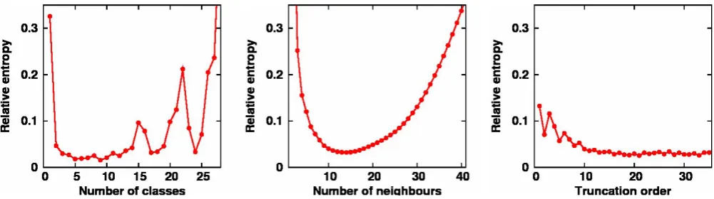
prior distribution0(k,θ )using these various approximations and computed the relative entropy (as a measure of the discrepancy between two pdfs, see for instance Bocquet et al., 2010) between the resulting transformed pdfs and the target transformed pdf N(0,1). Figure 2 (left panel) shows that there is indeed an optimal number of quantiles (q =9), which is close to the choice that we made in Fig. 1 (q=10). (Oscillations occur for largeq because the number of ensemble members in each class of the histogram becomes too small to produce an accurate estimation of the transformation.)
Gaussian mixture: Other estimates of the transforma-tion functransforma-tion can be obtained using more sophisticated nonparametric estimates of f (x), for instance by approxi-mating the unknown pdf by a mixture of Gaussian kernels (Izenman, 2008) rather than a mixture of uniform kernels (as in the histogram approximation). A common algorithm to estimate the Gaussian mixture from the available sample can be derived from the nearest neighbour method (e.g. Silverman, 1986; Izenman, 2008): each member of the sam-ple is used as the mean of one of the superposed Gaussian pdfs, with a variance equal to the variance of theq nearest neighbours. As in the histogram approximation, there is an optimalq below which spurious features are introduced in the pdf estimate, and above which significant features are smoothed out.
Figure 2 (middle panel) shows however that this optimalq
(minimizing the relative entropy) produces an estimate off (x)that is not better than the best histogram (even if the behaviour as a function ofq is more regular). Moreover, the numerical cost of the transformation, requiring numerical root-finding in the integral of the superposed Gaussian pdfs [to solve the equation F (x)˜ = ˜G(z)], would be much too high to be affordable in large size applications.
Polynomial development: Another way of constructing a direct approximation of the anamorphosis transformation (described in Wackernagel, 2003) is (i) to approximate
Fig. 2. Relative entropy between the transformation of the exact0(k,θ )andN(0,1), using various approximations of the transformation function: the histogram approximation (left panel), as a function of the numberqof classes in the histogram, the Gaussian mixture approxi-mation (middle panel), as a function of the numberqof nearest neighbours, the Hermite polynomial development (right panel), as a function of the numberqof superposed polynomials. In all 3 cases, the relative entropy is computed by numerical integration over the same interval
|z|<2.576, except in the 3rd case (polynomial development) for which the subintervals with zero density (due to the non-bijectivity of the approximation) have been removed.
x∈ [x(α),x(α+1)] where x(α), α=1,...,m is the ordered
sample (i.e. a step function instead of a piecewise linear function in the approximation above), (ii) to deduce the corresponding transformation as G−1[ ˜F (x)] =G−1(α/m)
forx∈ [x(α),x(α+1)], or reciprocally, to construct an
empir-ical anamorphosis transformation as F˜−1[G(z)] =x(α) for z∈ [G−1(αm−1),G−1(mα)] (i.e. again a step function, which is not bijective by construction), and (iii) to interpolate this empirical anamorphosis transformation by a limited development in Hermite polynomials (see Wackernagel, 2003, for more detail about this algorithm). Theq-th order Hermite development can be shown to be the best q-th order approximation (of the transformation function) in the least square sense (Wackernagel, 2003), but nothing guarantees that the polynomial interpolation will produce a bijective transformation, as it should be, so that ad hoc corrections must be supplied if problems occurs. (To avoid this problem, Simon and Bertino, 2009, linearly interpolate the step function instead of the development in Hermite polynomials.)
Figure 2 (right panel) shows the relative entropy between the transformed pdf obtained with this method and the ex-act pdf, as a function of the truncation orderq in the devel-opment of Hermite polynomials. Again, there exists a best truncation orderq=21, which is not more accurate than the histogram best estimate (shown on the left panel). These re-sults suggest that, with a moderate size sample (200 members in this example), it is not easy to do better than the simple histogram approximation, and that more sophisticated (and more expensive) algorithms, like the Gaussian mixture or the polynomial development, need a substantial increase in the sample size before producing a significant benefit.
2.3 Extensions of the algorithm
The algorithm described above is sufficient and well-conditioned as soon as (i) the cdf F (x) of every control variable is invertible (so that the quantiles of the ensemble are distinct), (ii) the range of possible value for every control variable is finite (between x1 and xp), and (iii) the size m of the ensemble is large enough to provide a reasonable approximation F (x)˜ of the marginal distributions. The purpose of this section is to examine what may be done if these 3 conditions are not verified.
Probability concentrations: A cdf F (x) is not invert-ible if it makes a vertical step at some valuex=xc, i.e. if
there is a probability concentration for x=xc, with finite probability: p(xc)=F (xc+)−F (xc−). In this case, several ensemble members may be equal to xc [mp(xc) members in average] so that a subset of the quantiles (between x˜l
andx˜u) may also be equal toxc, and the piecewise linear approximation of the anamorphosis transformation is no more bijective (zero denominator in Eq. 2). This occurs very often in practice, especially if there is a physical constraint on the value of the random variable, so that probability may concentrate on the constraint: sea temperature equal to freezing point, zero tracer concentration (see examples in Sects. 4, 5 and 7), ice fraction equal to 0 or 1 (see example in Sect. 6), ice velocity equal to 0 (no motion),. . .
The most direct solution to this problem (applied in all applications below, except in the Mercator applications in Sect. 6) is to transformxc to the middle of the step of the piecewise linear function: G˜−1[ ˜F (xc)] =21(x˜l+ ˜xu). A
preferable to restore the bijectivity of the transformation by introducing an artificial slope in the function. A simple way to do it is to replace the quantilesx˜l tox˜u (all equal toxc) by interpolating them betweenx˜l−1 andx˜u+1 (betweenx˜1 andx˜u+1 if l=1, or betweenx˜l−1 andx˜q if u=q). This
can improve the continuity and the quality of the linear estimates in the transformed space (see Sect. 6), at the price of a slight spreading of the backward transform around the concentration value xc (above xc if l=1, or below xc if
u=q).
Tails of the distribution: Since the range of possible values for the Gaussian random variableZ is between−∞ and+∞, the backward transformation in Eq. (3) must also specify how to transformz < z1andz > zq. If the range of
possible values for the original random variableX is finite betweenxmin andxmax, and fully resolved by the available ensemble (so that x˜1=xmin and x˜q=xmax), then we can be certain that the cumulated probability corresponding to
z < z1andz > zqis concentrated at x=xminandx=xmax, so that the backward transformation may be written:
ϕback(z)= ˜x1 for z < z1 (6)
ϕback(z)= ˜xq for z > zq (7)
But if the range betweenxminandxmax(possibly infinite) is not fully resolved by the available ensemble, a solution must be provided to map[−∞,z1]on[xmin,x˜1], and[zq,∞]on
[ ˜xq,xmax].
The most simple parameterization of the tails of F (x)
(used in all applications below) is to assume zero probabil-ity outside the range of the ensemble forecast (as in B´eal et al., 2010). Again, this corresponds to assuming that the cumulated probability corresponding toz < z1andz > zqis
concentrated atx=xminandx=xmax, so that the backward transformation is approximated by Eqs. (6) and (7). On the other hand, any x found outside of the interval [ ˜x1,x˜q] is
viewed as impossible and transformed as the closest value:
ϕforw(x)=z1 for x <x˜1 (8)
ϕforw(x)=zq for x >x˜q (9)
Parameterizing the tails of F (x) by probability concentra-tions atx˜1 andx˜q means that the resulting transformation
cannot be bijective outside of the interval[ ˜x1,x˜q]. However,
if the available ensemble is large enough and consistently sampled (without bias) from the prior probability distribu-tion, these tails must correspond to a very small cumulated probability. Moreover, if little is known about the extreme behaviour of the system, Eqs. (6) to (9) may be a safe way of avoiding any kind of extrapolation outside the range of values that has been explored by the ensemble.
More sophisticated assumptions about the tails of F (x)
can nevertheless be easily implemented. See for instance
Simon and Bertino (2009) for a Gaussian parameterization (requiring thatxminorxmaxbe infinite).
Sample enrichment: In many practical applications, it may be very expensive to increase the ensemble sizemuntil the accuracy of the approximation is sufficient to improve (or at least not deteriorate) the Gaussianity of the marginal distributions. In such circumstances, and providing that
F (x)is slowly varying in space, a better accuracy ofF (x)˜ at a given location x can certainly be obtained (for a moderate size m) by augmenting the sample that is available at x, with the samples that are available in the neighbourhood of x (possibly with a decreasing weight as a function of the distance from x). However, the definition of this neighbour-hood (which should decrease withm) introduces a subjective parameter in the algorithm, which can only be optimized by checking the accuracy of the results. This is why no enrichment of the sample is used in the applications below (except in the Mercator application in Sect. 6), where we preferred to stick to the theoretical formulation (converging form→ ∞) of separate transformations for distinct random variables (Wackernagel, 2003).
Finally, it is important to remark that such a spatial ex-tension of the sample is by no way necessary to ensure the spatial smoothness of the approximate solution described in Sect. 2.1. If all ensemble membersx(α)are spatially smooth,
their quantilesx˜k and thus the anamorphosis transformation
in Eqs. (2) and (3) will be spatially smooth as well (see ap-plications below), so that no spurious discontinuity is intro-duced in the multivariate probability distribution. On the contrary, one should certainly be careful enough to check that the sample extension described above does not smooth out real discontinuities (or sharp gradients) from the statistics. Again, what really matters to apply linear estimation meth-ods is that the joint probability distribution for all control variables, at every spatial location x, is better described by a multivariate Gaussian distribution if the nonlinear change of variables proposed in Eq. (2) is applied. It is precisely the purpose of the following examples to show that such local anamorphic transformations may yield a far better model for various kind of ocean uncertainties.
2.4 Effect on correlations
However, since the examples given in the following sections are mainly dedicated to illustrate the effect of anamorphic transformations on spatial correlations, it is certainly useful to provide first a summary of the theoretical background ex-plaining the effect that can be expected. For that purpose, we assume that we have two non-Gaussian random variables
dependence (in a general sense) between the random vari-ables remains unchanged, i.e. the reduction of entropy gained from the knowledge of the other variable (i.e. the mutual in-formation I) remains the same:
I (X1,X2)=H (X2)−H (X2|X1)=H (Z2)−H (Z2|Z1)
=I (Z1,Z2) (10)
which can easily be verified by introducing the change of variables in the definition of entropy [H (X2)] and condi-tional entropy [H (X2|X1)]. Consequently, it is only the effect of anamorphic transformations on linear correlations that we are going to investigate, since this is the only kind of correlation that can be described by a Gaussian model.
A first insight into this problem can easily be obtained by remarking that, if there exists separate bijective transforma-tions forX1 andX2 transforming their joint non-Gaussian distribution into a bi-Gaussian distribution for Z1 and Z2, then the anamorphic transformation given by Eq. (1) pro-vides the required transformations. This is obvious since the marginal pdfs of a bi-Gaussian distribution are both Gaus-sian, and the only backward anamorphosis (except for any unimportant additional linear change of variable) transform-ing the Gaussian marginal pdf forZ1andZ2 into the right marginal pdfs forX1andX2is the one given by Eq. (1). In this ideal case, the mutual information is related to the linear correlation coefficientρZ1Z2 between the transformed vari-ables (e.g. Cover and Thomas, 2006, chapter 8) by:
I (X1,X2)=I (Z1,Z2)= − 1
2ln(1−ρ 2
Z1Z2) (11)
A particular case of this ideal situation occurs if the vari-ableX1andX2 are perfectly correlated along a monotonic nonlinear curve (i.e. the ideal situation to estimateX2from an observation ofX1, but in which linear estimation methods can be very inaccurate). In this case, by transforming the two marginal pdfs into Gaussian pdfs, the anamorphic transfor-mations also transform the nonlinear curve into a straight line (so that the two marginal pdfs can be simultaneously Gaus-sian). The nonlinear dependence betweenX1andX2 (result-ing from their non-Gaussian behaviour) is fully transformed into a linear dependence, which is then perfectly described by the bi-Gaussian pdf (i.e. linear estimation methods be-come truly optimal). In this particular case, the linear corre-lation coefficient, which only imperfectly described the per-fect nonlinear dependence betweenX1andX2, is always am-plified by the transformation (|ρX1X2|<|ρZ1Z2| '1), as a di-rect consequence of the transformation of the nonlinear curve into a straight line. This first explanation thus covers all situ-ations in which|ρZ1Z2|is close to 1, because this means that all transformed values are aligned close to a straight line (as a result of the transformation of a nonlinear regression curve into a straight line). This kind of behaviour is what is ob-served for spatial correlations in most examples described in Sects. 3 to 7.
Nevertheless, it is important to stay aware that, in gen-eral, only the marginal distributionsp(Z1) and p(Z2)are ensured to be Gaussian, and that assuming thatp(Z1,Z2)is bi-Gaussian is only an approximation. This is why, in this case, it is much more difficult to make general mathematical statements about the transformation of linear correlations. A useful way to understand how linear correlations are modi-fied by the transformationX1,X2→Z1,Z2is to observe that the linear coefficient between the transformed variablesZ1 andZ2corresponds to a nonparametric measure of correla-tion between the original variablesX1andX2, because there is an abundant statistical literature explaining the advantages of nonparametric correlations as compared to linear corre-lations (Hollander and Wolfe, 1973; Corder and Foreman, 2009). In summary, the two main advantages are (a) that they are more adequate to see a nonlinear dependence be-tween random variables (for the same kind of reason as in the ideal case described above), and (b) that they are more ro-bust to the presence of outliers in the data. These two cases correspond to the situations in which the linear correlation can provide an inaccurate representation of the dependence between the random variables (as illustrated in the examples of Anscombe, 1973). And the basic reason underlying these two improvements is the derivation of variables that are iden-tically distributed (Z1andZ2are both normal in our case).
The oldest and most simple example of a nonparametric measure of correlation is the rank correlation (Spearman, 1904; Kendall, 1962), which is defined as the linear corre-lation between the rank of each member in the ensemble. Hence, this corresponds to computing a linear correlation be-tween uniform sets of integers bebe-tween 1 andm, which is thus close to computing a linear correlation after a uniform anamorphosis (i.e. with a uniform target pdf), instead of a Gaussian anamorphosis. (This is only approximate because, unlike uniform anamorphosis, the computation of the rank is not invertible, so that there is a small loss of information in the operation.) The close similarity between the rank corre-lation betweenX1andX2and the linear correlation between
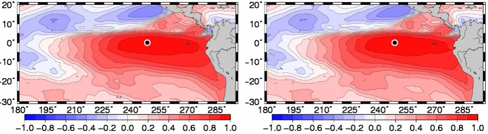
Fig. 3. SST horizontal correlation structure with respect to SST at 114◦W 0◦N (Eastern Equatorial Pacific), without anamorphosis (left panel), and after local anamorphosis transformations (right panel).
3 Mixed layer response to atmospheric forcing uncertainties
As a first example, we study the stochastic response of the ocean mixed layer to uncertainties in the atmospheric param-eters that are used to define the surface boundary condition of the ocean model (i.e. the momentum, heat and fresh water fluxes). In many respects, the ensemble model forecast that we use here to illustrate the effect of anamorphosis transfor-mations is similar to the ensembles that are used in Skan-drani et al. (2009) to estimate corrections in the atmospheric parameters using oceanic observations (without anamorpho-sis), because (i) we use the same low resolution global ocean configuration (ORCA2) of the NEMO-OPA model (Madec and Imbard, 1996), with a 2◦×2◦ ORCA type horizontal
grid and 31 z-coordinate levels along the vertical, and (ii) the random parameters perturbations are drawn from a Gaussian probability distribution with zero mean and a covariance de-rived from their natural variability. However, the ensemble that we describe here (performed by Meinvielle, 2011) is also somewhat different because (i) the reference atmospheric pa-rameters are obtained from the ERA-interim dataset instead of NCEP, with the objective (not discussed here) of esti-mating parameter corrections for long term model simula-tions (The DRAKKAR Group, 2007), (ii) the parameter per-turbations now include the wind, and are assumed constant over monthly periods, rather than weekly periods (to estimate lower frequency parameter corrections), and (iii) the covari-ance of the perturbations is set to the covaricovari-ance of the ERA-interim monthly means (from 1989 to 2007) for the 3 months surrounding the month of interest, rather than the full covari-ance of the parameter variability in Skandrani et al. (2009). In the following, we focus our study to the one-month and 200-member ensemble model forecast that is produced for January 2004, and we look at the mixed layer response, av-eraged over the one-month time period, in terms of sea sur-face temperature (SST), sea sursur-face salinity (SSS) and mixed layer depth (MLD).
Figure 3 shows for instance the resulting ensemble corre-lation structure with respect to SST at 114◦W 0◦N
(East-ern Equatorial Pacific), without anamorphosis (left panels), and after local anamorphosis transformations (right panels) based on the deciles of the ensemble forecast (as in Fig. 1). What we observe is that the SST horizontal correlation struc-ture is (almost) not modified by the local transformations. This occurs here because the ensemble model response to Gaussian parameter perturbations is already very close to Gaussian, so that the ensemble deciles for SST, at every lo-cation, are all remapped on the deciles ofN(0,1)along a straight line. Conversely, this means that the approximate algorithm described in Sect. 2, with piecewise linear trans-formations based on a histogram description of the proba-bility distributions, is accurate enough (with 200 members) to faithfully preserve the linear correlation structure between random variables that are already close to Gaussian. This Gaussian behaviour is also the reason why Skandrani et al. (2009) were able to infer relevant parameter corrections from SST (and SSS) using a Gaussian observational update algo-rithm (complemented by the truncated Gaussian assumption of Lauvernet et al., 2009, to avoid extreme and nonphysical corrections).
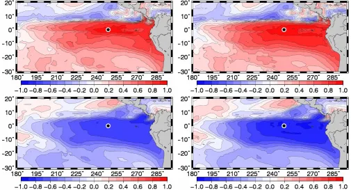
Fig. 4. MLD (top panels) and SST (bottom panels) horizontal correlation structure with respect to MLD at 114◦W 0◦N (Eastern Equatorial Pacific), without anamorphosis (left panels), and after local anamorphosis transformations (right panels).
Fig. 5. Scatterplot of MLD vs. SST at 114◦W 0◦N (Eastern Equatorial Pacific), without anamorphosis (left panel), and after local
anamor-phosis transformations (right panel).
scatterplot of MLD vs. SST at 114◦W 0◦N. As a
conse-quence, the joint distribution of MLD and SST cannot be bi-Gaussian, as visually obvious from the clear nonlinearity of the regression line (i.e. the line of maximum MLD probabil-ity for every given SST). In the transformed variables (Fig. 5, right panel), even if the marginal distribution for each vari-able is now close to Gaussian (by construction), the joint dis-tribution is still not bi-Gaussian (larger MLD dispersion for small SST than for large SST). But at least the regression
Fig. 6. Deciles of the ensemble for phytoplankton (top panels) corresponding (from left ot right) tork=0.2, 0.5 (median) and 0.8, and
illustration of one of the ensemble members (bottom panels): the phytoplankton map (left panel), the rank in the ensemble (middle panel), and the transformed map (right panel) after Gaussian anamorphosis.
estimation methods and the description of the final product (by the median and a set of quantiles, rather than the usual minimum variance estimate, which is not really meaningful in this case).
This first example already illustrates the two main con-clusions of this paper about the effect of local anamorphic transformations on the spatial correlation structure: (i) the transformation is accurate enough to faithfully preserve the correlation structure if the joint distribution is already close to Gaussian, and (ii) the transformation has the general ten-dency of increasing the correlation radius as soon as the spa-tial dependence between random variables becomes nonlin-ear. With the next examples, we further investigate the same effects in presence of the more complex and heterogeneous non-Gaussian behaviours that may occur in ecosystem or sea-ice models.
4 Ecosystem response to wind uncertainties
As a second example, we study the stochastic response of a coupled physical-biogeochemical model (CPBM) of the North Atlantic to uncertainties in the wind forcing. For that purpose, we use the same 200-member ensemble forecast as in B´eal et al. (2010): (i) the CPBM (originally devel-oped by Ourmi`eres et al., 2009) couples a 1/4◦ resolution circulation model of the North Atlantic (a Drakkar config-uration of the NEMO/OPA model, The DRAKKAR Group, 2007) with the LOBSTER (LOcean Biogeochemical Simu-lation Tools for Ecosystem and Resources, L´evy et al., 2005)
biogeochemical model, with 6 prognostic variables in the eu-photic layer: phytoplankton (PHY), zooplankton (ZOO), ni-trate (NO3), ammonium, detritus, and semi-labile dissolved organic nitrogen; (ii) the ensemble forecast is initialized at the beginning of the spring bloom on 15 April 1998, using the model simulation described in (Ourmi`eres et al., 2009); and (iii) the random wind perturbations are sampled from a Gaussian probability distribution, with zero mean and a covariance derived from the ERA40 variability (during the 3 months centered on 15 April, with a superimposed 4-day decorrelation times scale, see B´eal et al., 2010, for more details). However, whereas the study by B´eal et al. (2010) was exclusively focused on the multivariate response of the coupled model at given horizontal locations (with or with-out anamorphosis transformations, and for several forecast timescales between 1 and 30 days), we here complement their work, by documenting the effect of the local anamor-phic transformations on the horizontal correlation structure (in the 4-day forecast only).
In the ensemble forecast, the main impact of the random wind perturbations on the ecosystem results from the deep-ening and shallowing of the mixed layer, which modifies the nutrient supply and thus the primary production in the eu-photic layer. This mechanism produces a quite heteroge-nous response in terms of phytoplankton concentration, as illustrated in Fig. 6 by three deciles of the ensemble (corre-sponding tork=0.2, 0.5 and 0.8, top panels) and one of the
Fig. 7. Phytoplankton (top panels) and nitrate (bottom panels) horizontal correlation structure with respect to phytoplankton at 37.5◦W 50.8◦N (North Atlantic), as obtained for the original variables (left panels), their local rank in the ensemble (middle panels), and the transformed variables after Gaussian anamophosis (right panels).
the spring bloom has already started, like primarily the Gulf Stream pathway, the Irminger Sea and the Western half of the Labrador Sea, and secondarily, the Northern half of the North Sea, the Gulf of Lions and the Bay of Biscay. Con-versely, in the areas where the primary production is weak (as in the subtropical gyre and in the Norwegian Sea), it re-mains weak, whatever the wind perturbations.
Furthermore, one particular ensemble member (Fig. 6, bottom left panel) may be well below the median in some regions (e.g. in the Labrador Sea) and well above the median in other regions (e.g. in the Irminger Sea). This phenomenon is more obvious if we look at the rank of this ensemble mem-ber in the ensemble forecast (Fig. 6, bottom middle panel). More precisely, what is shown is the rank divided by the en-semble size (to be between 0 and 1), which corresponds to the local anamorphic transformation of the ensemble mem-ber using the uniform distributionU(0,1)as a target distribu-tion. For instance, a value below 0.2 means below the second decile (r2=0.2), a value below 0.5 means below the me-dian (r5=0.5), etc. In this figure, we can see immediately where this ensemble member is high or low with respect to the others (compare the rank in the Labrador Sea and in the Irminger Sea), even in regions where the dispersion of the ensemble is very small, as along the coast of Africa or in the Southern half of the North Sea. See also how the high rank region in the Irminger Sea (i.e. with a production well above the ensemble median) embeds indifferently areas of high pri-mary production and areas of low production, as a result of a strongly positive wind anomaly covering the whole region.
The rank may thus better translate the effect of a homoge-neous perturbation, which is masked in the original variable by the heterogeneity of the ecosystem dynamics. And from the local rank (Fig. 6, bottom middle panel) to the local Gaus-sian anamorphic transformation of the same ensemble mem-ber (Fig. 6, bottom right panel), there is nothing but a global anamorphosis transformingU(0,1)intoN(0,1). The figure thus looks very similar, with the same nonlinear change of variable at every grid point (we could have kept the same figure, with a nonlinear labelling of the colorbar).
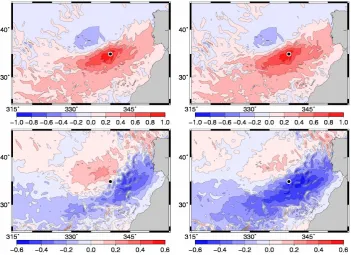
Fig. 8. Phytoplankton (top panels) and nitrate (bottom panels) horizontal correlation structure with respect to phytoplankton at 20◦W 35◦N (North Atlantic), without anamorphosis (left panels), and after local anamorphosis transformations (right panels).
between the two random variables (as illustrated in Fig. 5). The rank correlation was indeed introduced by Spearman (as explained by Von Mises, 1964) to produce this effect and thus to go beyond the linear correlation coefficient (of Pearson), as a measure of the (nonlinear) dependency between random variables. Furthermore, since the linear correlation structure after a local Gaussian anamorphosis is very similar to rank correlation (compare right and middle panels in Fig. 7), this explains why the correlation radius is generally increased by the transformation (compare with left panels, in which the area with a correlation above 80 % is about 26 % smaller for PHY and 35 % smaller for NO3). The same kind of phe-nomenon can be observed in Fig. 8, showing the same result at 20◦W 35◦N, except that the rank correlation is not shown anymore since it is always very similar to the linear corre-lation structure after Gaussian anamorphosis. However, we can see that here, the NO3 horizontal correlation structure (bottom panels) is deeply modified by the transformation, becoming more similar (in shape and extension, but with the opposite sign) to the PHY horizontal correlation struc-ture (top panels). This is also related to the improvement of the correlation between NO3and PHY at every horizontal lo-cation (which was described in B´eal et al., 2010), and further supports the idea that local anamorphic transformations may substantially increase the benefit that can be expected from ocean colour observations in the multivariate estimation of the state of the ecosystem.
5 Ecosystem response to ecosystem parameters uncertainties
Fig. 9. Phytoplankton (top panels) and nitrate (bottom panels) horizontal correlation structure with respect to phytoplankton at 11.7◦W 36◦N (North Atlantic), without anamorphosis (left panels), and after local anamorphosis transformations (right panels).
uncertainties after a 1-month ensemble forecast (instead of a 4-day forecast in the previous example).
Figure 9 shows for instance the PHY (top panels) and NO3 (bottom panels) horizontal correlation structure with respect to PHY at 11.7◦W 36◦N (in the Longhurst province west of Spain and North Africa), as obtained without anamorpho-sis (left panels) and after local anamorphoanamorpho-sis transformations (right panels), based on the deciles of the ensemble forecast. The first thing to observe is that the correlation is mostly sig-nificant inside the Longhurst province (materialized by the black line) with constant parameters perturbations, which means (i) that the ensemble size is sufficient to decorrelate independent behaviours, and (ii) that, even after 1 month, the effect of the parameter uncertainties is here mainly lo-cal (the main exceptions being the intense mesoslo-cale activity in the North-Western corner of the province, and the south-ward advection along the coast of Africa). However, inside the Longhurst province, the response of the ecosystem to the homogeneous parameters uncertainties is far from be-ing the same everywhere, as a result of the heterogeneity of the initial condition and physical forcing. It is also clearly nonlinear, in view of the strong impact of the anamorpho-sis transformation on the horizontal correlation structure. As in Fig. 8, the NO3correlation structure becomes very sim-ilar (with an opposite sign) to the PHY correlation struc-ture (Fig. 9, right panels), even though without anamorphosis (Fig. 9, left panels), the two variables were only weakly cor-related.
Fig. 10. Phytoplankton (top panels) and nitrate (bottom panels) horizontal correlation structure with respect to phytoplankton at 86◦W 23.8◦N (Gulf of Mexico), without anamorphosis (left panels), and after local anamorphosis transformations (right panels).
must be remembered that, even if these large long-range cor-relations are certainly meaningful, they cannot be expected to describe real model errors, because they correspond to a very simple assumption, in which parameter errors are as-sumed constant over the whole Gulf of Mexico.)
All these increases of linear correlation (or anticorrelation) contribute to simplify the Gaussian description of the uncer-tainties (in the transformed variables vs. the original vari-ables), by concentrating a larger fraction of the total variance in a smaller dimension subspace, thus reducing the number of degrees of freedom that must be controlled to obtain a given accuracy. This simplification is one of the main reasons for which local anamorphic transformations were so helpful in the work of Doron et al. (2011) to estimate the 39 un-known parameters from ocean colour observations (in a twin experiment approach, without localization of the ensemble covariance).
6 Modelling ice forecast uncertainties
In this section, we are moving to another class of examples, in which non-stochastic ensembles are used to describe fore-cast uncertainties. In many situations indeed, the forward model is too expensive to allow the explicit Monte Carlo ex-ploration of the uncertainties. Assumptions are then needed to produce the required ensemble of model states, using for instance an appropriate sample of the past system variability. The purpose of this section (and of Sect. 7) is to show that,
even in such a case, local anamorphic transformations may be useful to go beyond the Gaussian model.
As a first example of this kind, we study the non-stochastic ensemble description of sea-ice forecast uncertainties that is currently tested for assimilating sea-ice observations in the Mercator/MyOcean operational system. To construct the ensemble, it is assumed that the forecast uncertainties have the same statistics as the combined effect of the for-ward model short term and interannual variabilities. More precisely, to describe the uncertainties at a given date (e.g. 15 June 2011), we sample a past interannual free model sim-ulation (17 years, between 1991 and 2007) every 3 days in a running window of±66 days around that date (thus retain-ing 44 model states, every year), which make an ensemble of size m=17×44=748 model states. This assumption means that we do not try to resolve anything else than the seasonal cycle in the description of the uncertainties. This might look quite crude if we forget that this is applied to a 1/4◦ resolution global configuration of the NEMO model,
and already tested with a 1/12◦ resolution prototype. The
Fig. 11. Probability that the ocean is free of ice [p(f=0)], as computed from the non-stochastic ensemble for 15 March (left panel) and 11 September (right panel).
defined in the interval betweenf=0 (no ice) andf=1 (no free water).
Because of this bounded interval, it is already clear that the Gaussian model is not appropriate to describe uncertain-ties in ice concentrations. Moreover, the probability density function is usually maximum at one of these bounds (atf =1 in the middle of the ice pack, or at f=0 at the borders), or even at both (U-shaped pdf), which makes the Gaussian model even less appropriate. Furthermore, the two extreme values (f=0 orf=1) can often concentrate a finite proba-bility, which means that the cdf of ice concentration makes a step atf=0 orf=1 (as explained in Sect. 2.3). Figure 11 shows for instance the probability that the ocean is free of ice (f=0), as computed from the ensemble for 15 March (left panel) and 11 September (right panel). In practice, the value of this probability is computed as the fraction of the ensemble members for whichf =0. In this computation, we also ap-plied the sample enrichment method described in Sect. 2.3, by concatenating in the local description of the probability distribution all ice concentration values in a window of 9×9 grid points. The total ensemble size at each horizontal lo-cation is thus equal tom=81×748=60588. The effect of this enrichment of the ensemble is to slightly smooth the probability maps displayed in Fig. 11, but in view of the ap-proximations that are made in the construction of the original ensemble, there was no reason here to stay perfectly local, while the enrichment may be a good way of mitigating the inaccuracies that are related to the limited size of the
avail-able ensemble. In Fig. 11, the resulting probability increases fromp(f =0)=0 in the interior of the ice pack, where a zero ice concentration is impossible, top(f=0)=1 outside of the ice pack, where a zero ice concentration is certain (ac-cording to our assumption about the uncertainties). In the Arctic, it is also generally much larger in September (mini-mum ice extension) as compared to March, which shows the primary importance of resolving the seasonal cycle in the de-scription of the probability distributions.
Strictly speaking, in presence of such probability concen-trations (atf=0 in Fig. 11), a Gaussian anamorphosis trans-formation is not possible, since the cdf in Eq. (1) is not in-vertible. In our example, this means that several quantiles of the ensemble are equal tof=0, so that the piecewise linear approximation in Eq. (2) is not defined (zero denominator ifx˜k= ˜xk+1). This is why, in this example, we need to
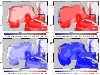
Fig. 12. Ice concentration horizontal correlation structure with respect to a reference location at 15◦W 75◦N (black dot) for 15 March (top panels) and 11 September (bottom panels), without anamorphosis (left panels), and after local anamorphosis transformations (right panels).
concentrated atf=0. It would of course be better to avoid any kind of approximation and to keep the exact descrip-tion of the probability concentradescrip-tions, but this is impossible with anamorphic transformations, and it is anyway useful for data assimilation to find new variables for which the Gaus-sian model is (at least approximately) valid, because it makes the observational update of the prior probability distribution (with linear formulas) numerically much more efficient. And to describe the marginal probability distributions for ice con-centrations, the above approximation is certainly much better than using a Gaussian model for the original variables (i.e. without anamorphic transformations).
Now, as in the previous examples, we turn to evaluating the effect of these local anamorphic transformations on the joint probability distribution by looking at the linear corre-lation structure. Figure 12 shows for instance the
Fig. 13. Time variability of the ensemble decilesrk=0.1,0.2,0.3,0.4,0.5,0.6,0.7,0.8,0.9 at 20◦W 35◦N (black dot in Fig. 14), as
obtained for phytoplankton (left panels) and nitrate (right panels) close to the surface (top panels) and at 41 m depth (bottom panels). The further from the median (rk=0.5, thick central curve), the thinner the curve.
As a secondary effect, the anamorphosis transformations also tend to remove the spurious correlations with the exterior of the ice pack (where the probability of a zero ice concentra-tion is close to 1). In the exterior of the ice pack, nearly all ice fractions are indeed equal to zero, so that the scatterplot with a point inside of the ice pack consists in a set of points aligned atf =0, except for a few outliers, which produce the spurious correlation. The shape of the scatterplot is thus like the example 4 in Anscombe’s quartet (Anscombe, 1973, Fig. 4), showing the effect of outliers on linear correlations in this typical case. By replacing the linear correlation by a nonparametric correlation, the anamorphic transformations help producing more robust correlations that are less influ-enced by the presence of outliers (see Sect. 2.4).
Hence, we can conclude that, in addition to significantly improving the description of the marginal probability dis-tributions for ice concentration (in the interval between 0 and 1), local anamorphic transformations are not detrimental to the description of the horizontal correlation structure, and may even help representing nonlinear dependences between distant ice behaviours.
7 Modelling ecosystem forecast uncertainties
As a second example of non-stochastic ensemble, we study the description of ecosystem forecast uncertainties that has been used in the MyOcean project (by Fontana et al., 2012) to assimilate ocean colour data in the NEMO/LOBSTER
1/4◦resolution CPBM (already described in Sects. 4 and 5) and produce a 9-year reanalysis (from 1998 to 2006) of the North-Atlantic ecosystem. The ensemble is constructed us-ing the same kind of assumption as in the previous example (in Sect. 6), by sampling an interannual free model simula-tion (7 years, between 1999 and 2005) every 2 days in a run-ning window of±30 days around the date of interest (thus retaining 30 model states, every year), which makes an en-semble of sizem=7×30=210 model states.
Figure 13 shows the deciles of the resulting ensemble as a function of time for phytoplankton (left panels) and nitrate (right panels) at 20◦W 35◦N (black dot in Fig. 14). This fully describes the approximate piecewise linear anamor-phosis transformation for this location, which is defined in Eqs. (2) and (3) by a remapping of this set of decilesx˜k on
the corresponding Gaussian decileszk. Consistently with our
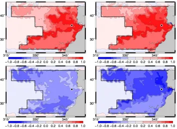
Fig. 14. Phytoplankton (top panels) and nitrate (bottom panels) horizontal correlation structure with respect to phytoplankton at 20◦W 35◦N (North Atlantic), without anamorphosis (left panels), and after local anamorphosis transformations (right panels).
becomes very low during the whole summer (between days 180 and 270), together with very low associated uncertain-ties (according to our assumption). To close the annual cy-cle, larger nitrate concentrations are then restored by vertical mixing during fall and winter (between days 270 and 45), when the primary production is reduced. During the whole cycle, the uncertainties on both concentrations (which are positive quantities) are clearly non-Gaussian, with the higher deciles (rk>0.5) being further away from the median than
the lower deciles (rk<0.5), especially during the
transi-tions between high and low concentratransi-tions. For instance, just before nitrates are fully depleted, the lower deciles and the median are already all close to zero, while the higher deciles are still very significant. These non-Gaussian ef-fects are first-order behaviours of the ecosystem uncertain-ties, which clearly illustrate the inadequacy of the Gaussian model, and the usefulness of our approximate piecewise-linear anamorphic transformations to improve the description of the marginal probability distributions, as well as their vari-ations in time along the annual cycle. Moreover, the dynam-ical characteristics of the spring bloom (amplitude, starting date,. . . ) are known to be very heterogeneous in the ocean, so that the associated uncertainties require local transforma-tions to be properly described. For instance, Fig. 13 (bottom panels) shows the seasonal cycle of the ensemble deciles at the same horizontal location, but at a different depth (41 m depth instead of the first model level). Here, the situation is completely changed with respect to the surface, because
the spring bloom is smaller, and nitrate is not fully depleted during summer. This implies that the non-Gaussian descrip-tion of the uncertainties must also be very different. See in particular the uncertainty in the nitrate concentration, which stays more symmetric around the median for the whole year. Moreover, as soon as the bloom is terminated in the surface layers (around day 180), more light becomes available at that depth, and a secondary bloom can occur during summer, to-gether with larger phytoplankton uncertainties as compared to surface layers. The improvement in the local description of the marginal distributions already explains why the ap-proximate anamorphosis algorithm described in Sect. 2 has been so useful in the work of Fontana et al. (2012) to improve ocean colour data assimilation.
PHY correlation structure, the first thing that we observe is the same kind of anisotropy as in Fig. 8, probably reflecting some basic horizontal structure of the ecosystem dynamics, even if the correlation radius is here much larger, because the wind variability (which has been used in Sect. 4 to parameter-ize the statistics of wind perturbations) has a smaller decor-relation scale than the ecosystem variability in this region. But despite of this difference, the effect of anamorphosis is the same: a substantial increase of the correlation radius, es-pecially in the direction in which the correlation radius is the smallest. This reduced anisotropy of the correlation struc-ture after anamorphosis indicates a nonlinear dependence be-tween the ecosystem behaviours across the frontal pattern.
Concerning the NO3correlation structure (Fig. 14, bottom panels), the horizontal pattern is not much changed by the lo-cal anamorphosis transformations, but the value of the cross-correlation with PHY is significantly increased. It is interest-ing to note that PHY and NO3are here positively correlated (they were anticorrelated in Fig. 8), which is the sign that, on 19 April (day 109 in Fig. 13), the short term variability dominates in the non-stochastic ensemble. This difference of behaviour between Figs. 8 and 14 can be better illustrated us-ing scatterplots of PHY at the reference point (20◦W 35◦N) vs. NO3at some distance from the reference (20◦W 33◦N), as shown in Fig. 15 for the correlation structure of Fig. 8 (top panels) and Fig. 14 (bottom panels), without anamorphosis (left panels) and with anamorphosis (right panels). In the first situation (corresponding to Fig. 8), the effect of wind perturbations is to introduce more or less mixing in the wa-ter column, so that the resulting perturbation of PHY and NO3tend to be anticorrelated (because of their opposit ver-tical gradient). And in the second situation (corresponding to Fig. 14), the model variability tends to positively correlate the PHY and NO3fluctuations. However, in both cases, we can observe in the scatterplots that the effect of the anamor-phic transformations (giving the same normalized Gaussian distribution to all marginal distributions) is to produce a scat-terplot with a more elliptical shape, which is a good indica-tion that the joint distribuindica-tion is also closer to a bi-Gaussian distribution. In these cases, it can be seen that the modifi-cation of the scatterplots results from the two properties of anamorphosis that were introduced in Sect. 2: (a) the lin-earization of a nonlinear dependence between the two vari-ables, and (b) the reduction of the effect of outliers (result-ing here from occasional extreme behaviours). In both cases, these two properties explain the increase of linear correlation from|ρX1X2| =0.07 to|ρZ1Z2| =0.43 in the top panels, and from|ρX1X2| =0.24 to|ρZ1Z2| =0.38 in the bottom panels.
However, a closer analysis of PHY-NO3cross-correlations in the last example shows that they are often changing sign after the bloom event, in a way that is very heterogeneous in space and time. In addition to the improvement of the marginal distributions illustrated in Fig. 13 (in particular, the zero probability associated to negative concentrations) and to the increase of the correlation radius illustrated in Fig. 14,
this ability of the scheme to adjust in space and time to local statistical behaviours is most probably one of the main rea-sons why it has been so helpful in the work of Fontana et al. (2012) to improve the estimate of NO3concentrations from ocean colour observations.
8 Conclusions
Many kinds of ocean uncertainties cannot be accurately de-scribed using a Gaussian model. This is particularly obvi-ous in the examples of ecosystem uncertainties (in Sects. 4, 5 and 7) and sea ice uncertainties (in Sect. 6), although this may also be true for ocean dynamics uncertainties (as in the mixed layer depth example in Sect. 3). On the other hand, in these examples, a general non-Gaussian description of the joint probability distribution would be impossible to iden-tify from a moderate size ensemble, because the uncertain-ties occur in too many dimensions (curse of dimensional-ity). Nevertheless, even with the available ensemble (a few hundred members in all examples described in the paper), it is certainly possible to go beyond the Gaussian assumption in the description of the marginal distribution for any indi-vidual random variable (including observation equivalents or indirect operational product). In this paper, we suggested that a very significant improvement can already be obtained with a very simple non-Gaussian description of the marginal distributions (histograms), based on a few quantiles of the ensemble (typically deciles, as in our examples). It is es-pecially interesting for large size applications, because it is (i) concise (described by qnvalues, if n is the number of variables, andq, the number of quantiles), (ii) efficient (com-putational complexity proportional tonmlogm, if mis the size of the ensemble), and (iii) often more accurate than the Gaussian description (based on the mean and standard de-viation). More importantly, this simple histogram descrip-tion can also directly be used to perform a piecewise linear change of variable (anamorphosis transformation), in such a way that each marginal distribution becomes approximately Gaussian. In these transformed variables, it is then possible to perform the ensemble observational update consistently with our simple description of the marginal uncertainties, by applying the standard Gaussian algorithm, providing that the ensemble correlation structure is preserved, or even im-proved, by the transformation.
Fig. 15. Scatterplots of PHY at the reference point (20◦W 35◦N) vs. NO3at some distance from the reference (20◦W 33◦N), corresponding to the correlation structures that are shown in Fig. 8 (top panels) and in Fig. 14 (bottom panels), without anamorphosis (left panels) and with anamorphosis (right panels).
variables corresponds to a nonlinear measure of correlation between the original variables, which is very similar to the rank correlation (Spearman). On the other hand, even if the method finds its full justification with a stochastic ensemble description of the uncertainties, the last two examples show that it may also be useful with the non-stochastic ensembles (resulting for instance from the system past variability) that are often used in present-day operational systems to reduce the numerical cost of data assimilation (until truly stochastic solutions become affordable). In both cases, the most impor-tant consequence for data assimilation of this increase in the correlation magnitude is a significant reduction in the num-ber of degrees of freedom in the uncertainties (in a Gaussian sense), so that a better estimation accuracy can be obtained from a given observation network. And from a more general point of view, this also means that it may sometimes be re-warding to put some time and numerical effort to improve the statistical description of the uncertainties, rather than giving too much confidence to oversimplistic assumptions.
Appendix A
Implementation issues
All examples of local anamorphic transformations described in this paper have been performed using specific tools that we have implemented in the SESAM public software2, ex-cept the example of Sect. 6, which has been perfomed using an independent implementation of the algorithm in the Mer-cator assimilation system (SAM2). More specifically, the re-sults displayed in Figs. 3 to 10, 13 and 14 have been obtained using four SESAM tools:
1. Computation of the quantiles of the input ensemble, with the SESAM commandline:
sesam -mode anam -inxbas[ens dir] -outxbasref[quant dir]
SESAM naming conventions), and [quant dir], a direc-tory containing as an input, the definition of the quan-tiles (an ASCII file with therk, k=1,...,q). From this,
SESAM computes the (local) quantiles of the ensemble ˜
xk, k=1,...,q(as a set of NetCDF files, in the directory
[quant dir]), linearly interpolating between successive ensemble members, if necessary.
2. Local anamorphic transformation of the input ensem-ble, with the SESAM commandline:
sesam -mode anam -inxbas[ens dir] -inxbasref[quant dir] -outxbas[aens dir] -typeoper +
where [ens dir] is a directory containing the input en-semble forecast, and [quant dir], a directory contain-ing the quantilesx˜k, k=1,...,qof the ensemble (as
ob-tained from the previous tool), and, as an additional in-put, the quantiles of the target distribution (an ASCII file with thezk, k=1,...,q). From this, SESAM computes
the transformed ensemble (as a set of NetCDF files, in the directory [aens dir]), by linearly interpolating be-tween thezk using Eq. (2). In this way, the
transforma-tion can easily be performed towards any target distri-bution (by just changing the ASCII file with thezk), in
particular towards the Gaussian distribution (as in most examples presented in this paper) or towards the uni-form distribution (using the same file for thezkand for
therk) as in the middle panels of Figs. 6 and 7. (The
backward transformation of Eq. (3) can be performed similarly by replacing the+ sign by a − sign in the commandline.)
3. Computation of the EOFs of the ensemble, with the SESAM commandline:
sesam -mode geof -inxbas[(a)ens dir] -outxbas[(a)eof dir]
where [(a)ens dir] is a directory containing the input or transformed ensemble, from which SESAM computes the EOFs (as a set of NetCDF files, in the directory [(a)eof dir]). This tool may be useful to obtain an or-thogonal basis of the linear subspace spanned by the (original or transformed) ensemble forecast, or to re-duce the rank of the ensemble covariance matrix (by discarding the directions with negligible variance). No rank reduction has been performed in the examples de-scribed in this paper.
4. Computation of the correlation structure, with the SESAM commandline:
sesam -mode corr -inxbas[(a)eof dir] -outvar[corr file] -incfg[cfg file]
where [(a)eof dir] is a directory containing the EOFs of the original or transformed ensemble (or the columns of any other square root of the ensemble covariance matrix), and [cfg file] is a configuration file describ-ing the reference variable (an ASCII file, with the name of the variable, and the grid coordinates). From this, SESAM computes the multivariate correlation structure with respect to the reference variable (as a NetCDF file [corr file] providing the corresponding column of the correlation matrix). This is the kind of result that is mostly displayed throughout this paper.
Hence, only four SESAM commandlines have been suffi-cient to produce all kinds of result that have been presented in this paper, for a variety of oceanographic applications. The first one (1) provides the histogram description of the marginal uncertainties. This is used by the second one (2) to perform the piecewise linear local anamorphic transforma-tion, as a preprocessing to any operation taking profit from Gaussianity, like the computation of EOFs (3), the diagnos-tic of the linear correlation structure (4) or the linear obser-vational update (not shown here). In this way, the same study can be easily repeated to any new oceanographic problem, to check if the same conclusions apply. In our view, the sim-plicity and modularity of the implementation is an additional argument speaking in favour of the approximate algorithm described in Sect. 2.
Acknowledgements. This work was conducted as a contribution to the MyOcean and SANGOMA projects funded by the EU (grants FP7-SPACE-2007-1-CT-218812-MYOCEAN and FP7-SPACE-2011-1-CT-283580-SANGOMA), with additional support from the ASSOCO project (ESA/ESRIN Contract Network 22408/09/I-EC) for M. Doron and CNES for M. Meinvielle. The calculations were performed using HPC resources from GENCI-IDRIS (Grant 2010-011279).
Edited by: J. Schr¨oter


![Fig. 11. Probability that the ocean is free of ice [p(f = 0)], as computed from the non-stochastic ensemble for 15 March (left panel) and11 September (right panel).](https://thumb-us.123doks.com/thumbv2/123dok_us/69227.1507541/15.595.57.539.61.321/probability-ocean-computed-stochastic-ensemble-march-september-panel.webp)