www.atmos-meas-tech.net/8/2195/2015/ doi:10.5194/amt-8-2195-2015
© Author(s) 2015. CC Attribution 3.0 License.
Comparison of GC/time-of-flight MS with GC/quadrupole MS
for halocarbon trace gas analysis
J. Hoker, F. Obersteiner, H. Bönisch, and A. Engel
Institute for Atmospheric and Environmental Science, Goethe University Frankfurt, Frankfurt, Germany
Correspondence to: A. Engel ([email protected])
Received: 5 November 2014 – Published in Atmos. Meas. Tech. Discuss.: 10 December 2014 Revised: 28 April 2015 – Accepted: 28 April 2015 – Published: 27 May 2015
Abstract. We present the application of time-of-flight mass spectrometry (TOF MS) for the analysis of halocarbons in the atmosphere after cryogenic sample preconcentration and gas chromatographic separation. For the described field of application, the quadrupole mass spectrometer (QP MS) is a state-of-the-art detector. This work aims at comparing two commercially available instruments, a QP MS and a TOF MS, with respect to mass resolution, mass accuracy, stability of the mass axis and instrument sensitivity, detector sensitiv-ity, measurement precision and detector linearity. Both mass spectrometers are operated on the same gas chromatographic system by splitting the column effluent to both detectors. The QP MS had to be operated in optimised single ion monitor-ing (SIM) mode to achieve a sensitivity which could compete with the TOF MS. The TOF MS provided full mass range information in any acquired mass spectrum without losing sensitivity. Whilst the QP MS showed the performance al-ready achieved in earlier tests, the sensitivity of the TOF MS was on average higher than that of the QP MS in the “opera-tional” SIM mode by a factor of up to 3, reaching detection limits of less than 0.2 pg. Measurement precision determined for the whole analytical system was up to 0.2 % depending on substance and sampled volume. The TOF MS instrument used for this study displayed significant non-linearities of up to 10 % for two-thirds of all analysed substances.
1 Introduction
With increasing evidence that anthropogenic chlorinated and brominated hydrocarbons can be transported into the strato-sphere and release chlorine and bromine atoms that can
signif-icantly facilitated by these advantages and the use of more narrow mass intervals is expected to reduce interferences and background noise. In addition, much higher data acquisition rates are possible using TOF MS, which is an advantage for fast chromatography. A TOF MS instrument can measure more than 10000 mass spectra per second. They are added up and averaged over a certain time period to yield the desired time resolution. The possibility of operating the TOF MS at high data rates is also of high interest for fast chromatogra-phy and narrow peaks, for which the operating frequency of quadrupole instruments (especially when measuring several ions) can be a limiting factor. The maximum time resolution for the TOF MS used in this study is 50 Hz. An increase in the data frequency will lead to decreased signal-to-noise levels. The data frequency must therefore be optimised to provide a sufficient number of data points per chromatographic peak while keeping the signal-to-noise level as high as possible. In contrast, a QP MS is a mass filter and will only measure one mass at a time. It needs to scan many individual masses sequentially to register a full mass spectrum. To achieve high sensitivity, QP MS are therefore often operated in single ion monitoring (SIM) mode in which the instrument is tuned to only one or a few selected ion masses and all other ions do not pass the quadrupole mass filter. Regardless of these limi-tations of the QP MS, it is widely used in analytical chemistry due to its stability, ease of operation, high degree of linear-ity, good reproducibility as well as sensitivity. Especially for atmospheric monitoring the advantage of obtaining the full mass information from the TOF instrument might allow ret-rospective quantifications of species which were not target at the time of the measurement. For this purpose the TOF MS must be well characterised (in particular with respect to lin-earity) and the calibration gas used during the measurements must contain measurable amounts of the retrospective sub-stances and be traceable to an absolute scale.
In this paper, a comparison of a state-of-the-art QP MS and a TOF MS is presented, with both mass spectrometers being coupled to the same gas chromatographic system. The instru-mental setup is described in Sect. 2. The GC QP MS system was characterised and used before for studies by Laube and Engel (2008); Brinckmann et al. (2012) and showed consis-tent results in the international comparison IHALACE (Inter-national Halocarbons in Air Comparison Experiment) with the NOAA (National Oceanic and Atmospheric Adminis-tration) network (Hall et al., 2013). We discuss the use of TOF MS in atmospheric trace gas measurements, in particu-lar for the detection and quantification of halocarbons, focus-ing on four substances: CFC-11, CFC-12, Halon-1211 and Iodomethane. These four substances cover the boiling point and typical concentration range of a total of 35 substances analysed. The six key parameters for atmospheric trace gas measurements discussed in this paper are (1) mass resolution and (2) mass accuracy of the detectors, (3) stability of the mass axis and instrument sensitivity, (4) detector sensitiv-ity represented by the limits of detection (LOD), (5)
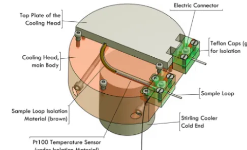
repro-Figure 1. Schematic of the cooling head. The aluminium cylin-der which contains the sample loop is placed on top of the Stirling cooler’s cold end. Electric connectors are located at each end of the sample loop for resistive heating.
ducibility of the measurement procedure and (6) the linearity of the detectors for varying amounts of analyte. The underly-ing experiments are described in Sect. 3 and their results are discussed in Sect. 4. Section 5 summarises the results of this work.
2 Instrumental
2.1 Preconcentration unit
calcu-late the preconcentration volume. After the preconcentration phase, the sample loop was heated resistively to+180◦C in a few seconds for instantaneous injection of the trapped an-alyte fraction onto the GC column. Desorption temperature was maintained for 4 min to clean the sample loop from all remaining compounds. All tubing (stainless steel) used for sample transfer between sample flask and preconcentration unit as well as preconcentration unit and GC was heated to 80◦C to avoid loss of analytes to the tubing wall.
2.2 Gas chromatograph
An Agilent Technologies 7890A GC with a Gas Pro PLOT column (0.32 mm inner diameter) was used for separation of analytes according to their boiling points. The column had a total length of 30 m, divided inside the GC oven into 7.5 m pre-column (backwards flushable) and 22.5 m main column. Purified helium 5.0 (Alphagaz 1, Air Liquide, Inc.) was used as carrier gas. The GC was operated with constant carrier gas pressure on both pre- and main column. The tempera-ture program of the GC consisted of five phases. (1) For the first 2 min, the temperature was kept at 50◦C. (2) Then the oven was heated at a rate of 15◦C min−1 up to 95◦C, (3) from thereon at 10◦C min−1 up to 135◦C and (4) then at a rate of 22◦C min−1 up to 200◦C. (5) The final tempera-ture of 200◦C was kept for 2.95 min. The resulting runtime was 17.95 min. The pre-column was flushed backwards with carrier gas after 12.6 min to avoid contamination with high-boiling substances. The gas chromatographic column was connected to the QP MS and the TOF MS using a Valco three-port union and two fused silica transfer lines. The trans-fer line to the QP MS had a total length of 0.70 m with an inner diameter of 0.1 mm, and the transfer line to the TOF MS had a total length of 2.10 m with an inner diameter of 0.15 mm. Based on the length, temperatures and inner diame-ters of the transfer lines, a split ratio of 63 : 37 (TOF MS : QP MS) was calculated. Using the ratios of the peak areas of the quadrupole when receiving the entire sample (TOF trans-fer line plugged) to those obtained in the split mode, a spilt ratio of 66 : 34 was calculated. We have adapted this latter value as it is based on actual measurements rather than cal-culations. All parts of the transfer lines outside the GC oven were heated to 200◦C.
2.3 Mass spectrometer
The two mass spectrometers in comparison were (1) an Ag-ilent Technologies 5975C QP MS and (2) a Markes Inter-national (former ALMSCO) Bench TOF-dx E-24 MS. Both MS were operated in electron ionisation mode with an ionisa-tion energy of 70 eV and ioniser temperatures of 230◦C. The QP MS was operated in SIM and SCAN mode (see Table 2 for more information). As the GC was operated in constant pressure mode, i.e. the head pressure of the columns were kept constant, the carrier gas flow into the two MS therefore
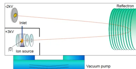
Figure 2. Scheme for the direct ion extraction of the Bench TOF-dx direct extraction (five technologies GmbH, G. Horner and P. Scha-nen, personal communication, 2014). The red dotted line represents a typical ion path.
varied according to the temperature ramp during each gas chromatographic run. Pressures inside the ion flight tubes of the MS therefore also varied; the TOF MS had a pressure range from 1.8×10⁻⁶ to 1.6×10⁻⁶hPa and the QP MS had a pressure range from 2.1×10⁻⁵to 1.8×10⁻⁵hPa. The Bench TOF-dx uses a direct ion extraction technique with an acceleration voltage of 5 kV. In contrast to many other TOF instruments, the ions are accelerated directly from the ion source into the drift tube instead of extracting them from the ion source and then accelerating them orthogonally to the extraction direction (orthogonal extraction). The direct extraction method in combination with the high acceleration energy orients the instrument towards a high sensitivity, espe-cially for heavier ions (five technologies GmbH, G. Horner and P. Schanen, personal communication, 2014). The TOF MS was set up to detect mass ranges from 45 to 500m/z; higher and lowerm/zwere discarded. The reason to discard ions withm/zratio below 45 was to eliminate a large part of the CO2which is trapped by our preconcentration method and can lead to saturation of the detector. A schematic of the Bench TOF-dx is given in Fig. 2. The spectra extraction rate was adjusted to 4 Hz to get a data acquisition rate comparable to that of the QP MS.
3 Experimental
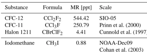
Table 1. Mixing ratios in ppt in the reference gas used in this work for the discussed substances.
Substance Formula MR [ppt] Scale
CFC-12 CCl2F2 544.42 SIO-05
CFC-11 CCl3F 250.79 Prinn et al. (2000) Halon 1211 CBrClF2 4.41 Cunnold et al. (1997)
Iodomethane CH3I 0.88 NOAA-Dec09 Cohan et al. (2003)
3.1 Measurement procedure and data evaluation To ensure measurement quality, both MS were tuned in reg-ular intervals (autotune by operating software) at least ev-ery 2 months but especially before sample measurements and/or characterisation experiments. Autotune options of both mass spectrometers were used without further manual adjustments. To increase the sensitivity and linearity of the TOF MS, its detector voltage was increased by 30 V, as de-scribed in Sect. 4.6. Additionally, a zero measurement (evac-uated sample loop), a blank measurement (preconcentration of purified Helium 5.0) and two calibration gas measure-ments were conducted to condition the system before ev-ery measurement series. At the end of evev-ery measurement series, another blank measurement was added. Every mea-surement series itself consisted of a calibration meamea-surement followed by two sample measurements (same sample). This sequence of three measurements was repeated n times de-pending on the type of experiment and then terminated by a calibration measurement. For characterisation experiments both calibration and sample measurements were taken from the same gas cylinder (reference gas, see description above) but treated differently in data evaluation, e.g. as a calibration or sample measurement. Chromatographic peaks were inte-grated with a custom designed software written in the pro-gramming language IDL. The peak integration is based not on a standard baseline integration method commonly used in chromatographic applications but on a peak fitting algorithm. For the results shown here Gaussian fits were used for peak integration. This software was also used for data processing by Sala et al. (2014) and described there. Noise calculation was performed on baseline sections of the ion mass traces of interest. The noise level was determined as the 3-fold stan-dard deviation of the residuals between data points and a second degree polynomial fit through these data points. This approach accounts for a drifting non-linear baseline. Other-wise, a non-linear baseline would cause an overestimation of the noise level. The integrated detector signal was divided by the preconcentration volume to get the detector response per sample volume. To account for detector drift during mea-surement series, the calibration meamea-surements bracketing the sample pairs were interpolated linearly. Thereby, interpolated calibration points are generated for each sample
measure-ment. The response for each sample was then derived by calculating the quotient between sample and corresponding interpolated calibration point. Experiments were conducted to analyse six key parameters (Sect. 3.2 to 3.7) important for measurements of halogenated trace gases in the atmosphere: mass resolution, mass accuracy, limits of detection, stabil-ity of the mass axis and instrument sensitivstabil-ity, measurement precision and reproducibility as well as detector linearity. 3.2 Mass resolution
The mass resolution (R) is defined as follows: R= m
1m, (1)
with1mbeing the full width at half maximum (FWHM) of the exact massmof the ion signal.
The mass resolution determines whether two neighbouring mass peaks can be separated from each other. It is consid-ered an instrument property, i.e. influenced only by internal factors like instrument geometry, ion optics, etc. The mass resolution of the TOF MS was calculated with its operating software ProtoTOF in a mass calibration tune. The QP MS was operated with MS Chemstation (Agilent Technologies, Inc.) which only processes unit mass resolution, independent of mass range.
3.3 Mass accuracy
The mass accuracy (δa) defined as
δa[ppm] = m−mm
mm×10−6
(2)
Table 2. Dwell time settings for given substance fragments in QP MS modes with a data frequency of≈3 Hz. SCAN mode (1): QP scanned from 50 to 500 u with 1.66 scans per second and a dwell time of 3.7 ms. Optimised (opti.) SIM mode (2): settings used for measurements on which LOD calculation was based, with 310 ms dwell time per ion and a scan rate of 3 scans per second. Operational SIM mode (3): default settings, used for reproducibility and linearity experiments with 3 scans per second.
Substance Fragment m/z QP SCAN mode Optimised (opti.) SIM mode Operational (oper.) SIM mode
[u] dwell time [ms] dwell time [ms]
for LOD calculation (1) for LOD calculation (2) for LOD calculation (3)
1.66 scans per second 3 scans per second 3 scans per second
CFC-12 CCl35F+2 85 50 to 500 u 50
CFC-11 CCl352 F+ 101 310 ms dwell time 70
Halon 1211 CCl35F+2 85 3.7 ms dwell time 100
Iodomethane CH3I+ 142 70
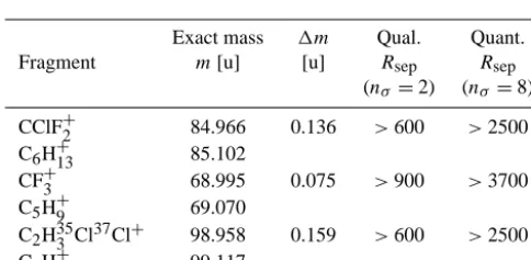
Table 3. Three exemplary halocarbon/hydrocarbon fragment pairs with equal unit mass but differing exact mass. The qualitative sepa-rating resolution (qual.Rsep) withnσ = 2 and the quantitative
sep-arating resolution (quan.Rsep) withnσ =8.
Exact mass 1m Qual. Quant.
Fragment m[u] [u] Rsep Rsep
(nσ=2) (nσ=8)
CClF+2 84.966 0.136 >600 >2500 C6H+13 85.102
CF+3 68.995 0.075 >900 >3700
C5H+9 69.070
C2H353 Cl37Cl+ 98.958 0.159 >600 >2500 C7H+15 99.117
3.4 Stability of the mass axis and instrument sensitivity To evaluate the stability of the two mass spectrometers with respect to sensitivity and accuracy of the mass axis, a repro-ducibility experiment was used. The relative difference be-tween the minimum and maximum detector response of the day and the 1σ standard deviation of all measurements over this day were taken as measures of the drift. For drift in mass accuracy over the day, the mean value and the 1σ standard deviation are given for the main masses for the following four compounds: HFC-134a (CF+3, 68.995 u), CFC-12 (CF352 Cl+, 84.866 u), CFC-11 (CF35Cl+2, 100.936 u,) and Iodomethane (CH3I+, 141.928 u). To evaluate the stability of the mass ac-curacy over a longer time period, the mass acac-curacy was cal-culated on measurement days with different time differences since the last mass calibration tune.
3.5 Limits of detection
The lowest amount of a substance that can reliably be proven is considered to be its LOD and serves as a measure for the sensitivity of the analytical system. Based on the assumption that a molecule fragment (f) can be detected when its
detec-Table 4. The difference of the minimal (Min) and maximal (Max) values in % in one reproducibility experiment for the relative re-sponse is shown with a 1σ relative standard deviation (RSD) over all measurements (20) on this day. In the comment line the trend of the calibration gas over the day is given.
Mass Substance Max−Min RSD Comment
spectrometer [ % ] [ % ]
TOF MS CFC-12 4 1.41 linear
QP MS CFC-12 4 1.28 linear
TOF MS CFC-11 5 1.32 linear
QP MS CFC-11 5 1.38 linear
TOF MS Halon-1211 7 1.97 linear
QP MS Halon-1211 1 0.63 linear
TOF MS Iodomethane 10 3.73 scatter
QP MS Iodomethane 5 1.92 scatter
tor signal height (Hfi) is equal to or higher than 3 times the signal noise (Nfi) on the adjacent baseline (signal-to-noise level (S/N) >3), a limit of detection for a fragment (fi) from an analyte substance (Si) with a mass (mSi) in the in-jected sample can be calculated as
LODSi =
3·Nfi·mSi Hfi
. (3)
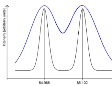
Figure 3. Schematic display of two different mass resolutions (blue and black curves). Two signals on masses 84.966 and 85.102 u with equal intensities demonstrate the mass separation with R=600 (blue curve) andR=3700 (black curve). Assuming Gaussian peak shapes for the signals,R=3700 separates both peak by 8σ (quan-titative separation) andR=600 separates them by only 2σ (quali-tative separation).
(up to six) in one scan with individual dwell times given in Table 2 and≈3 scans per second.
The LOD in pg and ppq were calculated for 0.28 L sample volume with respect to the split ratio (see Sect. 2.2) and then extrapolated to 1 L of ambient air.
3.6 Reproducibility and measurement precision The measurement precision describes the repeatability of a measurement. We determine the precision from the repro-ducibility (i.e. the standard deviation) of the measurements. The mean reproducibility is derived from dedicated multi-ple experiments designed to assess measurement precision (reproducibility experiment). Reproducibility was analysed over five measurement series, conducted on 5 different days, to give the mean measurement precision. Every experiment followed the procedure described in Sect. 3.1, with a total of 19 evaluated measurements of the same ambient air sample. A subset of the samples was treated as standard, the other part as unknown samples (two samples bracketed by two stan-dards). Every individual measurement of these five series was conducted with a preconcentration volume of 0.28 L of the reference gas. Two additional reproducibility experiments were conducted with a higher preconcentration volume of 1 L to assess the possible dependence of the reproducibil-ity on the preconcentrated sample volume. For each sample pair, the standard deviation of the relative response was cal-culated, summed up over all pairs and divided by the number of pairs to form the sample pair measurement reproducibil-ity of that measurement series. The described procedure was applied to all analysed substances and reproducibility exper-iments. The mean value of measurement reproducibilities is considered to be the measurement precision of the system for the respective substance and volume.
3.7 Detector linearity
Detector linearity was analysed in two linearity experiments by varying the default preconcentration volume of 0.28 L by factors of 0.33, 0.66, 1.25 and 2 (sample positions in the measurement sequence, see Sect. 3.1). As calibration mea-surements, the default preconcentration volume was used. For comparison, detector responses were calculated as the ratio of the area of a chromatographic peak (A) to the pre-concentration volume (V). All detector responses were nor-malised to 1 (relative detector response) by dividing them by the meanA/V of the calibration measurements. An ideally linear detector would show a relative response of 1 for any preconcentration volume used. The errors for the linearity measurements were derived as the 3-fold standard deviation given from reproducibility experiments.
4 Results and discussion 4.1 Mass resolution
If mass resolution is sufficiently high, it is possible to sep-arate mass peaks of equal unit mass but differing exact mass. This separation drastically enhances the possibility to identify specific molecule fragments and to reduce cross-sensitivity. For halocarbon analysis, it is interesting to sep-arate halogenated molecule fragments with exact masses typically below unit mass from other fragments with exact masses typically at or slightly above unit mass (e.g. hydro-carbon fragments). It could then be possible to reduce back-ground noise generated by interfering ion signals or even compensate co-elution of non-target species from the GC column. For quantitative analysis the separation of adjacent mass signals implicates a possible loss of signal area when both mass peaks are not fully separated. The imposed error, i.e. the peak area lost due to separation, should not decrease measurement precision and should therefore be lower than the targeted measurement precision, in our case 0.1 %.
For this purpose, the definition of a qualitative and a quan-titative separating resolutionRSep is introduced (see Fig. 3 for an illustration). Assuming a Gaussian peak shape (normal distribution) of the ion signal on the mass axis, a separation of two neighbouring signalsm1andm2(withm2> m1) by 8σ (SD, 4σ per peak) is considered a quantitative separation (less than 0.01 % loss of peak area) while a separation by less than 8σis considered to be only a qualitative separation. Fur-ther assuming that 1σ is approximately 1/2 FWHM (or 1/2 1mrespectively) and that1m1is not significantly different from1m2, one can estimateRSep(atm1orm2) for a known (m2−m1) difference:
Rsep= m1
1m1
= m1
2·(m2−m1) nσ
. (4)
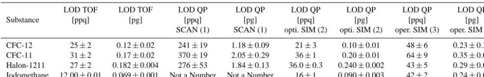
Table 5. The limit of detection (LOD) in ppq and pg of the substances CFC-12, CFC-11, Halon-1211 and Iodomethane in 1 L of air sample per detector. The dwell times and settings for the QP MS are given in Table 2. The given errors are 1σstandard deviation.
LOD TOF LOD TOF LOD QP LOD QP LOD QP LOD QP LOD QP LOD QP Substance [ppq] [pg] [ppq] [pg] [ppq] [pg] [ppq] [pg]
SCAN (1) SCAN (1) opti. SIM (2) opti. SIM (2) oper. SIM (3) oper. SIM (3)
CFC-12 25±2 0.12±0.02 241±19 1.18±0.09 21±3 0.10±0.01 48±6 0.23±0.30 CFC-11 31±2 0.17±0.02 370±19 2.05±0.29 36±1 0.20±0.01 64±9 0.35±0.05 Halon-1211 27±2 0.182±0.004 276±53 1.84±0.13 36.0±0.3 0.240±0.002 43±5 0.29±0.02 Iodomethane 12.00±0.01 0.069±0.001 Not a Number Not a Number 16±1 0.090±0.003 42±2 0.24±0.05
Table 6. The reproducibility (REP) for the QP MS and the TOF MS as a mean value of five measurement series with 20 measurements each and a preconcentration volume of 0.28 L. The given errors are 1σ standard deviation over five reproducibility experiments.
Substance Formula REP QP [ % ] REP TOF [ % ]
CFC-12 CCl2F2 0.56±0.31 0.56±0.18 CFC-11 CCl3F 0.45±0.26 0.54±0.23 Halon-1211 CBrClF2 1.56±0.52 0.94±0.39 Iodomethane CH3I 3.96±0.72 3.44±1.61
Table 7. The reproducibility (REP) for the QP MS and the TOF MS as a mean value of two measurement series with 20 measurements each and a preconcentration volume of 1.00 L. The given errors are 1σ standard deviation over two reproducibility experiments.
Substance Formula REP QP [ % ] REP TOF [ % ]
CFC-12 CCl2F2 0.22±0.10 0.23±0.09 CFC-11 CCl3F 0.14±0.03 0.16±0.00 Halon-1211 CBrClF2 0.60±0.05 0.55±0.21 Iodomethane CH3I 1.31±0.23 0.99±0.30
qualitative separating resolution. Table 3 shows some ex-amples for qualitative and quantitative separating resolu-tions required for separation of halogenated mass fragments from hydrocarbon molecule fragments with slightly different masses.
To separate e.g. the CClF+2 ion signal from the C6H+13 ion signal qualitatively, a resolution of 600 is necessary. For a quantitative separation, the mass resolution has to be R=3700 according to the definition of 8σ separation (see above). For the Bench TOF-dx, the calculated mass resolution was R=1000 at mass 218.985 u for the frag-ment C4F+9 in a mass calibration tune by the software Pro-toTOF. This allows a qualitative separation of two neigh-bouring mass peaks like the ones listed in Table 3, e.g. the separation of mass 84.966 u to mass 85.102 u. An exam-ple of a mass spectrum centred around 85 u is shown in Fig. 4 for a chromatogram of a typical ambient air sam-ple at a retention time of 11.35 minutes. Two mass peaks, one centred at 84.943 u (CH35Cl37Cl+), a fragment of the Trichloromethane (CHCl3) molecule and one with a mass
Figure 4. So-called 0.01 u mass spectrum of the substance Trichloromethane. Two mass peaks are shown. The higher one by mass 84.9 u is identified as the molecule fragment (CH35Cl37Cl+) and the other one by mass 85.1 u is an unidentified hydrocarbon peak.
slightly above unit mass, can be clearly distinguished. The higher mass is the result of an unidentified hydrocarbon peak eluting shortly before the Trichloromethane peak.
The resulting chromatogram centred at 11.3 minutes is shown in Fig. 5. Three different mass ranges were extracted from the raw data, the nominal mass range from 84.5 u to 85.5 u, the lower mass range from 84.7 u to 85.0 u and the higher mass range from 85.0 u to 85.3 u. When extracting the information centred around the unit mass range, a double peak is observed. An extraction of the lower mass range of the 85 u signal yields a much lower signal in the earlier elut-ing peak yet the signal cannot be reduced to baseline level. An extraction of the higher mass range of the signal gives a larger signal for the earlier eluting peak, but again the signal does not drop to baseline level.
4.2 Mass accuracy
While sufficient mass resolution is necessary for an unam-biguous separation of two mass peaks, mass accuracy is in addition needed for chemical identification of the detected ion. The better the mass accuracy, the lower the number of possible fragments that might be the source of the mass sig-nal. The mass accuracy for the Bench TOF-dx was found to be in a range of 50 to 170 ppm for a mass range from 69 u to 142 u. Mass accuracies for the analysed target masses were determined as follows: (100±60) ppm for mass 68.995 u, (80±50) ppm for 84.966 u, (120±50) ppm for 100.936 u and (130±40) ppm for 141.928 u. A correlation between the dis-played masses is observed: when the accuracy of one mass is decreased, the others are, too. There is no correlation given by the proximity of target masses to tuning compound (PFTBA, e.g. 68.995 u) masses. A suspected reason for the instability of the mass axis is the instrument temperature and resulting changes in material elongation. This is, how-ever, speculation. At a mass resolution of R=1000 at ion mass 85 u and an accuracy of 100 ppm, the mass difference between measured and exact mass would be 10 % of the FWHM of this mass peak (or 5 % at 50 ppm). The stability and absolute accuracy in the determination of the exact mass is thus not a significant additional limitation in the ability of the Bench TOF-dx to separate different ions (see Sect. 4.1). 4.3 Stability of the mass axis and instrument sensitivity A reproducibility experiment was used to evaluate the sta-bility of two detectors over a measurement series (typically 10 h). For that purpose, the minimum and maximum value of the detector response relative to all recorded responses and the 1-fold relative standard deviation of all recorded re-sponses were used (see Table 4).
For the substances CFC-11 and CFC-12 the drift of the sensitivity of the TOF MS and QP MS are on the same level. For the low concentrated substances, the drift of the TOF MS is higher than that of the QP MS.
For evaluating the stability of the mass axis, the drift over a day was calculated as mean accuracy and standard deviation (1σ). The stability over a long time period was observed over different days away from a mass accuracy tune. As shown in Sect. 4.2 the mass accuracy of the Bench TOF-dx was ob-served to be on the order of 50–170 ppm. Within this uncer-tainty no drift of the mass axis with time could be observed for periods of up to 19 days after the mass axis calibration. The stability and absolute accuracy in the determination of the exact mass is thus not a significant additional limitation in the ability of the Bench TOF-dx to separate different ions (see Sect. 4.1).
Figure 5. A chromatogram of an unidentified hydrocarbon peak (smaller one) eluting slightly earlier than the higher Trichloromethane peak. The nominal mass 85 u (black) shows a double peak. By choosing the lower mass range (84.7 u to 85.0 u; red) a lower signal for the unidentified hydrocarbon peak is ob-served, and by choosing the higher mass range (85.0 u to 85.3 u, blue) a lower signal for the Trichloromethane peak is observed.
4.4 Limits of detection
For halocarbon measurement, sensitivity is an important is-sue as atmospheric concentrations can be below 1 pg L−1 of ambient air, especially for newly released anthropogenic species. Table 5 shows the calculated LOD for the QP and the TOF MS for the four selected species with different mea-surement settings of the quadrupole MS detector.
for the different substances. For substances with high con-centration shorter dwell times are chosen, while the dwell time is increased for substances with low concentrations in order to increase the sensitivity. Only one ion is measured for most species in order to reach optimum sensitivity. As a consequence, limits of detection are higher in such mea-surements as in the optimised SIM mode. Respective LOD for the discussed dwell time settings are shown in Table 5.
In comparison to the QP MS, the TOF MS is up to 12 times more sensitive than the QP MS in the SCAN mode. In the optimised SIM mode with increased dwell times (2) for specific ion masses, limits of detection in quadrupole MS and time-of-flight MS are similar. During routine measurements (operational SIM mode (3)), the limits of detection of the TOF MS were up to a factor of 3 lower than those of the QP MS.
4.5 Reproducibility
A high measurement precision is required as it is of great importance to detect very small variability of halocarbons in the atmosphere, e.g. to characterise trends of highly per-sistent substances (Montzka and Reimann, 2011; Montzka et al., 2009; Vollmer et al., 2006). Table 6 shows exemplary reproducibilities for both instruments based on a preconcen-tration volume of 0.28 L. The reproducibility is rather similar for both MS, with values below 1 % for the species with high ambient air concentrations and therefore high signal-to-noise levels (CFC-12 and CFC-11). For the species with lower con-centration and lower signal-to-noise levels the reproducibil-ity of the TOF seems to be slightly but not significantly better (see Table 6).
The reproducibilities shown in Table 6 are based on mea-surements with a relatively small sample volume. Larger pre-concentration volumes should result in better reproducibili-ties as signal-to-noise levels are increased and error sources during sample preparation should become smaller relative to the sample volume. Therefore, two reproducibility experi-ments with a larger preconcentration volume of 1 L were per-formed. The results are shown in Table 7.
The increase of the preconcentration volume to 1 L yields a significant improvement of the measurement precision. The high signal-to-noise species CFC-12 and CFC-11 now show reproducibilities below 0.3 % for the QP and for the TOF. For the low signal-to-noise species Halon-1211 and CH3I the re-producibilities are improved by a factor of up to 4 for the TOF MS and by a factor of up to 3 for the QP MS, with the TOF instrument showing better reproducibilities. As for the TOF MS, the detector itself was found to be a limita-tion to higher preconcentralimita-tion volumes as it showed satu-ration effects for some analysed ions already at 0.5 L pre-concentrated sample. For example, CFC-12 had to be evalu-ated on mass 87 u (relative abundance: 32.6 %) and CFC-11 on mass 103 u (relative abundance: 65.7 %) (NIST, 2014) as both main quantifier ion masses (85 and 101 u) showed
satu-ration in the respective retention time windows. This satura-tion reflects the limited dynamic range of the analog to digital converter (memory of 8 bits) used in the Bench TOF-dx. 4.6 Linearity
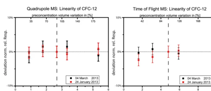
For the calculation of the mixing ratio of a measured sub-stance, its detector signal has to be correlated with the sig-nal of the same substance in a calibration measurement with known mixing ratio. If the detector behaves linearly, this cor-relation is linear and the calculation of the mixing ratio is straight forward. As mixing ratios in different air samples might vary to a great extent (e.g. diurnal variations of short-lived substances) (Sala et al., 2014; Derwent et al., 2012; Law and Sturges, 2011), a linear detector simplifies data evalu-ation to a great extent. Furthermore, retrospective analysis of substances that were not identified at the time of mea-surement is possible without an unknown error due to de-tector non-linearity. Figures 6 and 7 show linearity plots for the QP MS for the CFC-11 and CFC-12 based on two lin-earity experiments. The QP MS showed a linear behaviour within the measurement errors (3-fold measurement repro-ducibility for the respective substance). This linearity test in-cludes possible effects of the preconcentration unit (quantita-tive adsorption and desorption) as well as the determination of the preconcentration volume, the GC and data processing (signal integration). Figures 6 and 7 illustrate results from the two linearity experiments for the TOF MS. For CFC-11 (Fig. 6) a deviation from linearity for small preconcentra-tion volumes of nearly 10 % is observed, while detector be-haviour is close to the ideal value for high preconcentration volumes. The red curve was derived based on the standard detector voltage of−2244.8 V. An decrease of the detector voltage by−30 V brought slight improvements but did not solve the issue. Figure 7 shows a linearity plot for the sub-stance CFC-12. For CFC-12 the detector is considered to be linear within the error bars. Both detectors compared in this work depend on the same sample preparation and separation steps before detection. As measurement reproducibilities of QP MS and TOF MS were not significantly different, the di-rect comparison is possible without limitations. The exam-ples displayed for the QP MS and the TOF MS are two of 35 substances measured and analysed. The QP MS showed lin-ear behaviour for all substances within the uncertainty range. The non-linearity of the TOF-MS was highest for the low preconcentration volume (33 %, 0.09 L) with deviations of
Figure 6. Linearity graphs of CFC-11 (CFCl+2 fragment) based on two different linearity experiments (red and black plots in each graph). Primaryxaxis (lower): mass on column in ng. Secondaryxaxis (upper): preconcentration volume variation in % versus a default precon-centration volume of 0.28 L (dashed line).Y axis: deviation from the normalised relative detector response versus the detector response of the default preconcentration volume). For every preconcentration volume, the relative response should be one in case of a linear detector behaviour (dashed line). The error bars show the three-fold measurement precision, on the left-hand side for the QP MS and on the right-hand side for the TOF MS. The second linearity experiment (black) of the TOF MS was conducted with an decreased detector voltage (−2274.8 V instead of−2244.8 V).
Figure 7. Same figure as Fig. 6 for the substance CFC-12 (CF2Cl+fragment).
found for the QP MS but only for some species in the TOF MS. If the detector does not behave linearly, the relationship between the integrated peak area and the atmospheric con-centration has to be approximated by a fit function. In order to generate this fit function, additional measurements with varying preconcentration volumes are necessary before each measurement series. This procedure was found to be neces-sary for the TOF MS. It lengthens measurement series, im-plies an additional error source and requires additional time for data processing.
5 Conclusions
A Markes International Bench TOF-dx was compared to an Agilent Technologies 5975 QP MS with respect to the measurement of halogenated trace gases in the atmosphere. Both detectors ran in parallel (66:34 split) after cryogenic
to a factor of 12 higher than the LOD of the TOF MS. LOD of the TOF MS are lower by factors of up to 3 (Table 5) in com-parison to the QP MS with operational SIM mode settings used for routine measurements. In the SIM mode with only one quantifier (optimised SIM mode) the TOF MS is similar to the QP MS. In that respect, the TOF MS with its very high sensitivity and full mass range information provides a con-siderable advantage compared to a QP MS. The reproducibil-ity of both instruments was found to be on an equal level with slightly better reproducibilities of the QP MS at high signal-to-noise levels and slightly better reproducibilities of the TOF MS for low-concentrated species. Regarding detec-tor linearity, the Bench TOF-dx in its current configuration could not compete with the QP MS. A high degree of linear-ity is, however, necessary for high accuracy measurements in trace gas analysis. The encountered non-linearities neces-sitate a correction which adds an error source, especially when there is a large concentration difference between sam-ple and calibration measurement. It furthermore complicates measurements as well as data evaluation. For other applica-tions where concentration variability is significantly higher than the non-linearity of the detector, the observed detector non-linearities might not be of such high relevance. In con-clusion, the TOF MS does show advantages with respect to mass resolution and sensitivity without losing the full mass spectra information. Persisting non-linearities are a big dis-advantage but might be conquered in the future by develop-ments in detector electronics. With reduced non-linearities, TOF MS could well be the technology of the future for the analysis of halogenated trace gases in the atmosphere, de-spite the significantly higher costs of the TOF MS in com-parison to QP MS instruments. These conclusions are only valid for the Markes International Bench TOF-dx E-24 MS and atmospheric trace gas measurements and might turn out differently for another field of research or another TOF MS.
Acknowledgements. The authors would like to thank five
tech-nologies GmbH for the technical support of the Bench TOF-dx, Laurin Hermann for the mechanical design and construction of the cooling head. J. Hoker thanks the European Community’s Seventh Framework Programme (FP7/2007–2013) in the InGOS project under grant agreement 284274 for financial support.
Edited by: R. Koppmann
References
Aydin, M. and De Bruyn, D. J. and Saltzman, E.: Preindustrial at-mospheric carbonyl sulfide (OCS) from an Antarctic ice core, Geophys. Res. Lett., 29, 73, doi:10.1029/2002GL014796, 2002. Brinckmann, S., Engel, A., Bönisch, H., Quack, B., and At-las, E.: Short-lived brominated hydrocarbons – observations in the source regions and the tropical tropopause layer, Atmos.
Chem. Phys., 12, 1213–1228, doi:10.5194/acp-12-1213-2012, 2012.
Cohan, D. S., Sturrock, G. A., Biazar, A. P., and Fraser, P. J.: Atmospheric Methyl Iodide at Cape Grim, Tasmania, from AGAGE Observations, J. Atmos. Chem., 44, 131–150, doi:10.1023/a:1022481516151, 2003.
Cooke, K. M., Simmonds, P. G., Nickless, G., and Make-peace, A. P. W.: Use of Capillary Gas Chromatography with Neg-ative Ion-Chemical Ionization Mass Spectrometry for the Deter-mination of Perfluorocarbon Tracers in the Atmosphere, Anal. Chem., 73, 4295–4300, doi:10.1021/ac001253d, 2001.
Cunnold, D. M., Weiss, R. F., Prinn, R. G., Hartley, D., Sim-monds, P. G., Fraser, P. J., Miller, B., Alyea, F. N., and Porter, L.: GAGE/AGAGE measurements indicating reductions in global emissions of CCl3F and CCl2F2in 1992–1994, J. Geophys. Res., 102, 1259–1269, doi:10.1029/96jd02973, 1997.
Derwent, R. G., Simmonds, P. G., O’Doherty, S., Grant, A., Young, D., Cooke, M. C., Manning, A. J., Utembe, S. R., Jenkin, M. E., and Shallcross, D. E.: Seasonal cycles in short-lived hydrocarbons in baseline air masses arriv-ing at Mace Head, Ireland, Atmos. Environ., 62, 89–96, doi:10.1016/j.atmosenv.2012.08.023, 2012.
Farman, J. C., Gardiner, B. G., and Shanklin, J. D.: Large losses of total ozone in Antarctica reveal seasonal ClOx/NOxinteraction, Nature, 315, 207–210, doi:10.1038/315207a0, 1985.
Hall, B. D., Engel, A., Mühle, J., Elkins, J. W., Artuso, F., Atlas, E., Aydin, M., Blake, D., Brunke, E.-G., Chiavarini, S., Fraser, P. J., Happell, J., Krummel, P. B., Levin, I., Loewenstein, M., Maione, M., Montzka, S. A., O’Doherty, S., Reimann, S., Rhoderick, G., Saltzman, E. S., Scheel, H. E., Steele, L. P., Vollmer, M. K., Weiss, R. F., Worthy, D., and Yokouchi, Y.: Results from the International Halocarbons in Air Compari-son Experiment (IHALACE), Atmos. Meas. Tech., 7, 469–490, doi:10.5194/amt-7-469-2014, 2014.
Ivy, D. J., Arnold, T., Harth, C. M., Steele, L. P., Mühle, J., Rigby, M., Salameh, P. K., Leist, M., Krummel, P. B., Fraser, P. J., Weiss, R. F., and Prinn, R. G.: Atmospheric histories and growth trends of C4F10, C5F12, C6F14, C7F16and C8F18, Atmos. Chem. Phys., 12, 4313–4325, doi:10.5194/acp-12-4313-2012, 2012.
Jordan, A., Haidacher, S., Hanel, G., Hartungen, E., Märk, L., See-hauser, H., Schottkowsky, R., Sulzer, P., and Märk, T. D.: A high resolution and high sensitivity proton-transfer-reaction time-of-flight mass spectrometer (PTR-TOF-MS), Int. J. Mass Spec-trom., 286, 122–128, doi:10.1016/j.ijms.2009.07.005, 2009. Kim, Y.-H. and Kim, K.-H.: Ultimate Detectability of Volatile
Or-ganic Compounds: How Much Further Can We Reduce Their Ambient Air Sample Volumes for Analysis?, Anal. Chem., 84, 8284–8293, doi:10.1021/ac301792x, 2012.
Kundel, M., Huang, R.-J., Thorenz, U. R., Bosle, J., Mann, M. J. D., Ries, M., and Hoffmann, T.: Application of Time-of-Flight Aerosol Mass Spectrometry for the Online Measurement of Gaseous Molecular Iodine, Anal. Chem., 84, 1439–1445, doi:10.1021/ac202527a, 2012.
Laube, J. C. and Engel, A.: First atmospheric observations of three chlorofluorocarbons, Atmos. Chem. Phys., 8, 5143–5149, doi:10.5194/acp-8-5143-2008, 2008.
Röck-mann, T., Schwander, J., Witrant, E., Mills, G. P., Reeves, C. E., and Sturges, W. T.: Distributions, long term trends and emissions of four perfluorocarbons in remote parts of the atmosphere and firn air, Atmos. Chem. Phys., 12, 4081–4090, doi:10.5194/acp-12-4081-2012, 2012.
Laube, J. C., Newland, M. J., Hogan, C., Brenninkmeijer, C. A. M., Fraser, P. J., Martinerie, P., Oram, D. E., Reeves, C. E., Röckmann, T., Schwander, J., Witrant, E., and Sturges, W. T.: Newly detected ozone-depleting substances in the atmosphere, Nat. Geosci., 7, 266–269, doi:10.1038/ngeo2109, 2014. Law, K. S. and Sturges, W. T. L. A.: Global Ozone Research and
Monitoring Report – Chapter 2, WMO, Geneva, Switzerland, 2011.
Lee, J. M., Sturges, W. T., Penkett, S. A., Oram, D. E., Schmidt, U., Engel, A., and Bauer, R.: Observed stratospheric profiles and stratospheric lifetimes of HCFC-141b and HCFC-142b, Geo-phys. Res. Lett., 22, 1369–1372, doi:10.1029/95gl01313, 1995. Miller, B. R., Weiss, R. F., Salameh, P. K., Tanhua, T.,
Gre-ally, B. R., Mühle, J., and Simmonds, P. G.: Medusa: A Sam-ple Preconcentration and GC/MS Detector System for in Situ Measurements of Atmospheric Trace Halocarbons, Hydrocar-bons, and Sulfur Compounds, Anal. Chem., 80, 1536–1545, doi:10.1021/ac702084k, pMID: 18232668, 2008.
Molina, M. J. and Rowland, F. S.: Stratospheric sink for chloroflu-oromethanes: chlorine atomc-atalysed destruction of ozone, Na-ture, 249, 810–812, doi:10.1038/249810a0, 1974.
Montzka, S. A. and Reimann, S. L. A.: Global Ozone Research and Monitoring Report – Chapter 1, WMO, Geneva, Switzer-land, 2011.
Montzka, S. A., Hall, B. D., and Elkins, J. W.: Accelerated increases observed for hydrochlorofluorocarbons since 2004 in the global atmosphere, Geophys. Res. Lett., 36, L03804, doi:10.1029/2008gl036475, 2009.
NIST: National Institute of Standards and Technology: Mass Spec-tral Search Program for the NIST/EPA/NIH Mass SpecSpec-tral Li-brary, Gaithersburg, MD, USA, 2014.
Prinn, R. G., Weiss, R. F., Fraser, P. J., Simmonds, P. G., Cunnold, D. M., Alyea, F. N., O’Doherty, S., Salameh, P., Miller, B. R., Huang, J., Wang, R. H. J., Hartley, D. E., Harth, C., Steele, L. P., Sturrock, G., Midgley, P. M., and McCulloch, A.: A history of chemically and radiatively important gases in air deduced from ALE/GAGE/AGAGE, J. Geophys. Res., 105, 17751–17792, doi:10.1029/2000jd900141, 2000.
Sala, S., Bönisch, H., Keber, T., Oram, D. E., Mills, G., and Engel, A.: Deriving an atmospheric budget of total organic bromine using airborne in situ measurements from the western Pacific area during SHIVA, Atmos. Chem. Phys., 14, 6903–6923, doi:10.5194/acp-14-6903-2014, 2014.
Solomon, S.: Progress towards a quantitative understand-ing of Antarctic ozone depletion, Nature, 347, 347–354, doi:10.1038/347347a0, 1990.
Vollmer, M. K., Reimann, S., Folini, D., Porter, L. W., and Steele, L. P.: First appearance and rapid growth of anthropogenic HFC-245fa (CHF2CH2CF3) in the atmosphere, Geophys. Res. Lett., 33, L20806, doi:10.1029/2006GL026763, 2006.
Vollmer, M. K., Miller, B. R., Rigby, M., Reimann, S., Mühle, J., Krummel, P. B., O’Doherty, S., Kim, J., Rhee, T. S., Weiss, R. F., Fraser, P. J., Simmonds, P. G., Salameh, P. K., Harth, C. M., Wang, R. H. J., Steele, L. P., Young, D., Lunder, C. R., Hermansen, O., Ivy, D., Arnold, T., Schmidbauer, N., Kim, K.-R., Greally, B. R., Hill, M., Leist, M., Wenger, A., and Prinn, R. G.: Atmospheric histories and global emissions of the anthropogenic hydrofluorocarbons HFC-365mfc, HFC-245fa, HFC-227ea, and HFC-236fa, J. Geophys. Res., 116, D08304, doi:10.1029/2010jd015309, 2011.