www.ocean-sci.net/8/81/2012/ doi:10.5194/os-8-81-2012
© Author(s) 2012. CC Attribution 3.0 License.
Ocean Science
Sea surface temperature anomalies, seasonal cycle and trend
regimes in the Eastern Pacific coast
A. Ramos-Rodr´ıguez1,3, D. B. Lluch-Cota1, S. E. Lluch-Cota1, and A. Trasvi ˜na-Castro2
1Programa de Ecolog´ıa Pesquera, Centro de Investigaciones Biol´ogicas del Noroeste, S.C., La Paz, Mexico
2Departamento de Oceanograf´ıa F´ısica-Unidad La Paz, Centro de Investigaci´on Cient´ıfica y Educaci´on Superior de Ensenada,
Ensenada, Mexico
3Universidad Tecnol´ogica del Mar de Tamaulipas Bicentenario, La Pesca, Tamaulipas, Mexico
Correspondence to: A. Ramos-Rodr´ıguez ([email protected])
Received: 10 May 2011 – Published in Ocean Sci. Discuss.: 25 May 2011
Revised: 10 October 2011 – Accepted: 13 December 2011 – Published: 15 February 2012
Abstract. We used the extended reconstruction of sea face temperature (ERSST) to analyze the variation of sur-face temperature and the seasonal cycle along the coast of the eastern Pacific (60◦N–60◦S, 61 pixels alongshore) from 1950 to 2010 (732 months). First, we analyzed the monthly anomalies and looked for a relationship of such anomalies with total solar irradiance (TSI) and then the Regime Shift Detector (RSD) was applied to detect possible temperature regimes in the series. Afterwards, we calculated a yearly temperature range per pixel (amplitude of seasonal cycle) and through the subtraction of a latitudinal theoretical curve of temperature based on solar irradiance, the residuals of the seasonal cycle were obtained. The results showed an al-most complete spatial synchrony and dominance of negative anomalies from 1950 to mid-late 1970’s, with a switch to near-zero and positive anomalies that lasted up to late 1990’s when a new shift to negative values was detected. Such a shift lasted until the early 2000’s when positive anomalies appeared again but there was a change to negative anoma-lies in the late 2000’s. These results were supported by the RSD. The TSI variability shows a clear relationship with that of sea surface temperature anomalies and with the regime changes. This is probably due to a difference in the amount of energy received from the sun. Comparing the “cool regime” versus the “warm regime”, the second one received 0.39 % more energy (approximately 3×10⁸J m−2) from the sun. Seasonal cycles show larger ranges at northern lati-tudes (>40◦N), northern tropical-temperate transition zone (20◦–26◦N) and in the tropical-equatorial band (0◦–30◦S). The smallest ranges occur at 0◦–16◦N and 50◦–60◦S. The residuals (seasonal minus the theoretical curve) indicated a clear modulation due to advection by ocean currents.
1 Introduction
are highly influenced by physical variables such as winds and currents, all of which have an effect on SSTs.
Incoming radiation from the sun is the main energy source and is fundamental in influencing terrestrial climate. Vari-ations in the energy from the sun reaching the Earth’s sur-face is often assumed to be the source of climate disparities (Reid, 1991). The spatial and temporal variation in solar ra-diation due to solar altitude produces seasonal variation in temperatures, precipitation and many other aspects of the at-mospheric environment (Moran and Morgan, 1997). Season-ality even changes on longer time scales, mainly due to alter-ations in Earth’s orbital eccentricity and the tilt of planet’s ro-tational axis, varying on recognized cycles of approximately 41 k.y. and 100 k.y. respectively, and known as Milankovitch cycles (Milankovitch, 1941; Bennett, 1990).
On shorter time scales the radiation from the sun changes and has different cycle lengths. Among them we can find the Sunspots or Schwabe cycles (11 yr; Dean, 2000), Hale cycles (22 yr; Dean, 2000), Gleissberg cycles (88 yr; Braun et al., 2005; Peristykh and Damon, 2003), DeVries-Suess cycles (210 yr; Wagner et al., 2001), Hallstat or Hallstadtzeit cy-cles (∼2400 yr; Charv´atov´a, 2000; Vasiliev and Dergachev, 2002). Such variability in the radiation from the sun has an effect on the climate dynamics of the Earth and it is the main motor (Rind, 2002). Here we study the variability along the coast of the eastern Pacific and we compare it with the vari-ability in solar radiation. The hypothesis is that solar cy-cles should be present in records of different oceanographic variables modulated by other important processes such as the ocean currents.
The work is organized as follows. The following section describes the data and methodology used for its analysis. Section 3 discusses our results and a final section is dedicated to summarize our findings and for the concluding remarks.
2 Methodology
2.1 Sea surface temperature data and total solar irradiance data
For SSTs we used the extended reconstruction of sea sur-face temperature data set (ERSST). This is a database with a latitudinal and longitudinal spatial resolution of 2◦by 2◦ for each data point (pixels) and a time resolution of one month. For the analysis we selected pixels from the east-ern Pacific coast at 60◦N to 60◦S and only the pixels near-est to the coastline (61 pixels in total). ERSST data was generated from NOAA’s Historical Merged Land-Ocean Sur-face Temperature Analysis, version 3b (http://www.ncdc. noaa.gov/oa/climate/research/sst/ersstv3.php) and it includes data from January 1950 to December 2010, for a total of 732 months. The data in ERSST starts in 1854 but we de-cided to use only the above-mentioned period because the reported confidence interval for uncertainty for the
quasi-global average for 1950 onwards is of 0.1 °C. Improved fit procedures are also included for this period along with the omission of satellite observations due to the larger residual bias of such observations (Smith and Reynolds, 2003, 2004; Smith et al., 2008). The total solar irradiance data (TSI) was obtained from the SOLARIS working group web page hosted by the Physics of the Middle Atmosphere Group of the Freie Universit¨at of Berlin (http://www.geo.fu-berlin.de/ en/met/ag/strat/forschung/SOLARIS/Input data/). Here they include data for the period 1880–2004. Such data is cal-culated with the use of observational data and proxies. It includes corrections for wavelength-dependent degradation common to measurements of TSI. A more detailed descrip-tion of these estimates can be found in Lean et al. (1997), Lean (2000) and Lean et al. (2005).
To determine the exact length and timing of every cycle the Cyclic Descent Method was used (Bloomfield, 1976). The latter method is useful to define the cycles present within a time series and fits a polynomial model that can be employed to forecast.
2.2 Monthly anomaly analysis
For the SST data, the monthly anomalies for each 2◦ by 2◦ coastal pixel were calculated by obtaining a mean of all months in the database resulting in an annual mean time series per pixel. This was then subtracted from individual monthly values in the time series.
In order to detect the presence of a SST regime shift in the different time series we used the Regime Shift Detector (RSD, Rodionov, 2004; Rodionov and Overland, 2005). The RSD is a useful tool to detect abrupt changes in a time se-ries by t-test analysis of either the mean or variance, and it is useful also since it can detect a shift with a minimum delay and not to be biased by long intervals when the observations remain above or below the overall mean value (red noise). Here the RSD was used with a significance level of 90 % (p <0.1), cut-off length of 60 month and Huber’s weight pa-rameter of 1. For the red-noise estimation, the Inverse Pro-portionality with 4 corrections (IP4) method was selected, using a sub-sample size of 39. Before applying the RSD a data pre-whitening was carried out (Rodionov, 2006). With the parameters above mentioned, we expect this method will detect a SST regime at least 5 yr long.
2.3 Seasonal amplitude cycle analysis
Jacobs et al. (2004). First, we obtain the solar declination for a given year using,
δt=·sin((dt−(21+28+31))· π 182.5)·
π
180 (1)
where, δt is the solar declination, is the Earth’s axial tilt
(23.44◦) andd
t is time in Julian days. To obtain the solar
al-titude or azimuth (α) series for a particular latitude we used, αt=arcsin(sin(Lat)·sin(δt)+cos(Lat)
·cos(δt)·cos(Yt))·
180
π (2)
where,Latis a given latitude in radians andYt is the hour of
the day. For every latitude in the study (pixel),αwas com-puted, and then the solar irradiance for such latitude (IrrLat|t)
was calculated as IrrLat|t=sin(αt·
π
180)·Irrnet (3)
whereI rrnet is the amount of net solar irradiance received
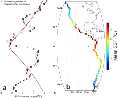
by the Earth’s surface (344 W m−2). We assumed an albedo of 0.3, hence the net solar irradiance used was 240.8 W m−2. The amplitude of the solar irradiance for each pixel (latitude) was obtained calculating the statistical range. This results in a theoretical latitudinal solar irradiance amplitude series (the amplitude value of solar irradiance for every pixel), which was used to compute regressions against their corresponding latitudinal mean SST seasonal amplitude series, which was calculated averaging the 61-yr SST amplitude series for each pixel (see Sect. 2.2), resulting in one mean SST amplitude value for every pixel (latitude) used in this study. The regres-sion was carried out in two steps: (1) from equator to 60◦N and, (2) from equator to 60◦S, resulting in a theoretical curve of latitudinal SST amplitude based on solar radiation (ampli-tude of the solar irradiance, red line in Fig. 1a).
3 Results and discussion
3.1 Meridional coastal variability: mean seasonal SST cycle and theoretical seasonal cycle based on solar irradiance curve
Figure 1a compares the annual mean SST range with the the-oretical seasonal temperature amplitude obtained from the ir-radiance cycle. This is shown for all coastal stations along the eastern Pacific. The statistical temperature range (maxi-mum – mini(maxi-mum) was calculated for every year in the data base. From 60◦to 56◦N in the region of the Alaska Current the seasonal cycle is 0.6 to 1 °C larger than the theoretical curve (TC). This is because this current is relatively warm and tends to increase the amplitude of the seasonal cycle. From 54◦ to 46◦N the mean SST range is close to the TC with differences less than 0.47 °C, most of them above the TC. This is thought to occur here because this region does
not have coastal upwelling sites and the California Current is found far from the coast. From 44◦to 30◦N is an area influ-enced by both the California Current and coastal upwelling. This is a temperate zone with a seasonal SST range of about 5–6 °C, nevertheless upwelling and California Current make this area cooler and more homogeneous, thus reducing the seasonal cycle and the SST range falling below the TC (0.45– 1.5 °C) with smaller differences in the latitudinal band 36◦– 34◦N. From 20◦to 26◦N the SST range is above that of the TC with values ranging from 1 to 2 °C and the largest differ-ences are found at 24 to 26◦N. Here the increase in seasonal SST range is due to the influence of tropical waters in the late summer and the presence of either the California Current or coastal upwelling lowering the coastal SSTs most of the year. The latitudinal band from 18◦N to 2◦N, which includes the eastern Pacific warm pool and north equatorial region, shows values close to the TC with differences no larger than 0.5 °C. As mentioned by Fiedler and Talley (2006), this warm band marks a thermal equator where the amplitude of the seasonal cycle is low. To the south, from the Equator to 28◦S we find the Humboldt or Peru Current region and intense coastal up-welling. This region is embedded in a tropical area and it should have a smaller SST range (around 2–3 °C) but due to the cold current and the upwelling the seasonal cycle is much greater (>6 °C). Consequently, the range is above the TC (values between 0.8–5.1 °C) with largest differences in the upwelling region between 4◦and 12◦S (4 to 5.1 °C). From 30◦S and to the south the mean SST range diminished pro-gressively. The difference of TC and average annual SST range over the 61 yr was lower at both 42◦S and 58◦S be-ing 1.2 °C and 5.15 °C lower, respectively. This is attributed to the influence of the Circumpolar Current and its extension to the north along the American coast (see also Sect. 3.3). Table 1 summarizes results shown above.
Mean SSTs showed a latitudinal gradient (Fig. 1b) with cooler temperatures at higher latitudes (coolest at 60◦S, 4.1 °C), as expected, and warmer temperatures near the equa-tor with the warmest SST north of the equaequa-torial region, from the 6◦–18◦N (27◦–28.5 °C) including the coast of the eastern Pacific warm pool (∼6◦–14◦N).
3.2 SST monthly mean anomalies, solar irradiance and Regime Shift Detector (RSD)
Fig. 1. (a) Mean latitudinal SST range for the selected pixels for the same period (black circles) and the theoretical SST range derived from
solar irradiance (red line). (b) Coastal stations (pixels) selected for the study with their mean SST for the 61 yr in the data base.
Table 1. Observed SST range, expected SST range, range difference and likely cause of such difference for seven latitudinal bands
found in the study. AC = Alaska Current, CC = California Current, EPWP = eastern Pacific warm pool, HC = Humboldt or Peru Current, CirC = Circumpolar Current.
Latitudinal band Observed Expected Difference Alteration due to 60◦–56◦N 8.26 7.57 0.69 AC
46◦–54◦N 7.13 6.94 0.19 CC away from coast 44◦–30◦N 4.73 5.69 −0.96 CC and upwelling
28◦–20◦N 5.52 4.22 1.29 CC, upwelling and tropical waters 18◦–2◦N 2.22 2.49 −0.27 Tropical waters and EPWP 0◦–28◦S 6.15 3.01 3.14 HC and upwelling 30◦–60◦S 3.96 6.43 −2.48 HC and CirC
was used (described in the methods section). This method is useful to define the cycles present within a time series and fits a polynomial model that can be employed to forecast the behaviour of a periodic component of the signal (2a, blue line,R2=0.78). The position of the start/end of each solar cycle was determined using this method and in Fig. 2 it is marked by black horizontal lines.
irradiance of the whole TSI series with minimum/maximum values of 1365.3/1366.3. The next two solar cycles lasted 10.5 each. The first one goes from January 1976 to July 1986 and the second from August 1986 to December 1996. The minima and maxima for both solar cycles are almost identi-cal, around 1365.4 and 1367.1, respectively. The remaining portion of series showed an incomplete period of increasing TSI trend.
In the following two panels of the Fig. 2 we show the SST anomalies and the regime shift detector applied to it. Nega-tive values of SST anomalies (Fig. 2b) dominated the period of 1950 to 1978 (SST regime 1 in 2c). Zero and positive anomalies dominated from 1979 to 1999 (SST regime 2 in 2c) and mostly weak anomalies from 2000 onwards (SST regime 3 in 2c). During first SST regime negative anoma-lies of 2 °C were common and only during El Ni˜no Southern Oscillation (ENSO) events (1957–1958, 1965–1966, 1968– 1969, 1972–1973, 1976–1977) is that near-zero or positive anomalies could be observed. During each ENSO event the intensity of the anomaly and its zonal extent are an indica-tion of the strength of individual occurrences. In most ENSO events, positive anomalies in the Southern Hemisphere range from the equator to about 16◦S. However, during some of the more intense ENSO events (v.g. 1957–1958) positive anoma-lies extend poleward to 30◦S and to 60◦N. Mid-intensity ENSO events resulted in a weaker response in the North-ern Hemisphere. During SST regime 2 (warm), from 1979 to about 1999, there was a clear dominance of near zero to positive anomalies with the only exception of the negative anomalies associated to negative ENSO (La Ni˜na) events. The strongest ENSO events of the whole series occurred during this warm SST regime, for instance during 1982– 1985 and 1997–2000 events. Such events have the widest zonal extent. In the 1997–1998 event, positive anomalies were recorded along the coast from 56◦S to 60◦N. The sec-ond SST regime shift occurred around 1998–1999, after the strongest ENSO event recorded in this time series. First, a shift back towards negative anomalies occurred, lasting about 6 yr. Then a brief near-zero to warm-anomaly period oc-curred in 2003 only to switch again to negative anomalies around 2007–2008. The main features of this period are: a) the weak character of the anomalies throughout the coastal region andb) the lack of strong ENSO events. These brief and weak events are similar to the El Ni˜no-Modoki class of ENSO events. Such behaviour has been described as a con-sequence of climate change by Ashok and Yamagata (2009). The behaviour of the total solar irradiance curve (2a) is consistent with the regimes described by the SST anomaly curves (2b). During the cool SST regime (1950 to 1978, as seen in 2b and 2c two full solar cycles took place. The first solar cycle is short and reaches the highest TSI values of the two. The second solar cycle is an elongated cycle with comparatively lower TSI maximum. This shows a clear rela-tionship with the SST anomalies. The maximum of the first solar cycle occurred during the El Ni˜no 1957–1958 and
dur-ing 1964–1975 the TSI reached a minimum and the period was dominated by negative anomalies. This TSI cycle is also the longest of the whole series, lasting 11.5 yr in total. As pointed out by Friis-Christensen and Lassen (1991) longer sunspot cycles have a relationship with cooler temperatures on the planet due to weaker solar activity.
The area below the curve is the energy received in the pe-riod of integration. To compare the energy received during successive pairs of solar cycles we computed the area below the curves. The first integration is carried out for two consec-utive cycles, from 1954 to 1975 (a total of 22.5 yr), and the second also for two consecutive cycles, from 1976 to 1996 (a total of 21 yr). The difference between the area below the TSI curves of the first and second SST regimes is of about 3×10⁸J m−2. This is equivalent to about 0.39 % more en-ergy received during the warm period compared to the cool period. This is a significant difference. Variations in total so-lar energetic output, as determined over time scales for which reliable climatic data are available, are small (less than about 0.1 %). Such percentage corresponds to a change of irradi-ance of approximately 1 W m−2outside the atmosphere (or 0.2 W m−2 averaged over Earth’s surface) between periods of maximum and minimum activity and over a full solar cy-cle (see for instance Haigh, 1996).
Furthermore, peaks in solar forcing increase the energy in-put to the upper ocean, increasing the latent heat flux (mois-ture) into the atmosphere, and moisture produced this way is carried by the trade winds towards the convergence zones where precipitation occurs. This intensified precipitation strengthens the Hadley and Walker circulations in the tro-posphere, with an associated increase in trade wind strength capable of increasing the strength of equatorial ocean up-welling and of lowering equatorial SSTs (Meehl et al., 2009). A consequence of this lowering of SSTs and increased up-welling is a positive feedback due to enhanced subsidence producing fewer clouds in the eastern Pacific that allow even more solar radiation to reach the ocean surface. There-fore, during shorter sunspot cycles (increased solar activ-ity), there is an increase in SSTs in the tropics and subtrop-ics that can help explain the higher temperatures observed during regime 2. This statement can be corroborated when observing Cold Tongue Index, which usually increases dur-ing higher temperatures of positive ENSO events or positive phases of Pacific Decadal Oscillation (Mantua et al., 1997).
towards a positive phase agrees with the first regime shift de-tected in the present work which switched the whole basin to warm conditions. As pointed out by Gershunov and Barnett (1998), some studies suggest that ENSO influences on cli-mate are strongly dependent on the phase of the PDO, such that the canonical El Ni˜no and La Ni˜na patterns of climate anomalies are most likely to occur during years in which ENSO and PDO extremes are in phase (i.e., with warm PDO coincident with El Ni˜no, and cool PDO coincident with La Ni˜na). During second regime (warm), the strongest ENSO events of the series were recorded, which is another resem-blance between PDO and the present work. It is worth noting the synchrony of regime shifts in this work and PDO phases, which indicates a deep coupling of the climatic system in the whole basin.
The regime shift detector (RSD) was applied to the SST anomalies (Fig. 2c). What makes this method useful is the use of a statistical test which includes a measure of the level of significance. This is very useful to detect if there is any meaningful change in the mean or variance of the time se-ries. The Hovm¨oller diagram of the RSD corroborates what was previously stated (Fig. 2c). There was a basin-scale SST regime shift around the year 1978 from cooler to warmer conditions. This SST regime shift occurs along the whole basin, with the exception of the region from 4◦S to 16◦– 18◦N where the regime shifts happened a little later, around mid-1980’s. The warm event from 24◦S to 60◦N in late 1950’s is related to the occurrence of the 1957–1958 ENSO event.
The SST regime changes to cool conditions in the late 1990’s. This occurred along the whole basin and it might have been triggered by la Ni˜na 1999–2001. This event started in late 1998 and lasted through 2000 with negative anomalies observed even during 2002.
3.3 Seasonal cycle amplitude and RSD
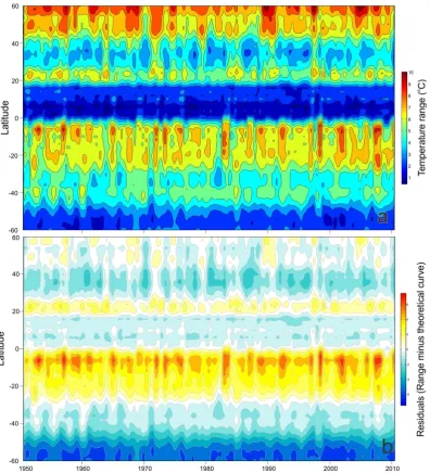
The Hovm¨oller diagram of the temperature amplitude (TA) and temperature residual (TR = range – theoretical curve of solar radiation, TC, see the methods section) are shown in Fig. 3a and 3b respectively. It is important to notice that latitudinal TA is caused by seasonal changes in solar radia-tion; meanwhile changes in TR are likely caused by physical processes such as ocean currents capable of modifying the phase of the seasonal warming/cooling cycle due to solar ir-radiance.
TA in Fig. 3a clearly denotes a latitudinal gradient ex-plained by the SST mean latitudinal range (Fig. 1a). TA was always larger than 7 °C in the mid- to high-latitudes (from 40◦N northwards), diminishes to a minimum of 2–4 °C from 28◦ to 40◦N, increasing again when it reached the tropi-cal transition zone (from 20◦ to 26◦N) and in the tropical to equatorial band the SST range was very small (less than 3 °C). In the southern hemisphere the larger SST ranges oc-curred in the equatorial to subtropical band (south of 0◦ to
26◦S) reaching up to 10 °C. Only the extreme south showed again a small range similar to that observed in the equator.
It is worth noting that ENSO events have a strong effect over the seasonal cycle, amplifying it or reducing it (Tren-berth, 1997; Galanti and Tziperman, 1999; Neelin et al., 2000). For example in the El Ni˜no 1997–1998 the effect dif-fered along the coast. From the equator southwards to 30◦S the presence of the Humboldt Current results in a reduction of the TA of 2 to 3 °C. Northwards along the coast the TA was amplified in the subtropical to tropical transition (20◦ to 26◦N) and in the mid- to high-latitude (40◦N and north-wards) due to the poleward propagation of the ENSO signal. After El Ni˜no event, La Ni˜na acted in exactly the opposite way. It amplified the SST range southwards of the equator and reduced it north of it.
When subtracting the TC from the TA (Fig. 3b) the resid-uals (TR) indicate how the temperature range is affected by other factors than merely solar radiation. After this calcula-tion the results indicates that ocean currents are the physical factors most important in influencing SST.
Fig. 2. Total solar radiation (a), Hovm¨oller diagram of the SST monthly anomalies (b) and the same type of diagram for RSD applied to SST
monthly anomalies (c). The colorbar in 2c represents the mean value for the regime detected trough RSD in the same units as SST (°C).
northernmost region (46◦–60◦N) is characterized by a sea-sonal cycle slightly larger than expected (up to∼2 °C), al-though it shows variability with negative values dominating in some periods. This is because this zone is influenced by the Alaska Current, known to be a warm current, and this
Fig. 3. Hovm¨oller diagram of the SST range (TA, (a)), and the residuals (TR) calculated from subtracting the theoretical curve from the
range (b).
The ocean currents play an important role in the distribu-tion of heat and momentum in the earth; in this case they alter the SST range near the coast by distributing the en-ergy received at other latitudes. Trenberth and Caron (2001) showed different estimates of derived ocean heat transport for some oceans. They showed calculated values for the “World Ocean” at 24◦ of 1.5–2.0 PW (Petawatt = 1015W), such values indicate the importance of the heat transport by currents.
4 Conclusions
In this study, during the last 61 yr two shifts to different “tem-perature regimes” were detected along the coast of the east-ern Pacific. This was carried out through analysis of monthly SST anomalies and using statistical tools, such as the regime shift detector (RSD). We found that the SST regimes were clearly related to the solar activity, particularly to the amount of TSI and length and intensity of sunspot cycle.
0.39 % more energy received during the warm SST regime compared to the cooler SST regime. Although a great per-centage of the energy received at the top of the atmosphere is lost due to dispersion, refraction, reflection, etc. The re-maining energy enters the climate system and the loss of about 0.39 % during the cool SST regime is not a negligi-ble amount. Another factor influencing incoming radiation from the sun in climatic regimes is the length of solar cycles that is longer during the cool SST regime (22 yr combined) than the remaining two cycles in the series (21 yr combined); while the second cycle of the cool SST regime (1964–1975) received the least amount of energy of the series. Hence, it is possible that these combined factors, less energy received due to reduced solar activity because of the longer cycles and less irradiance, caused the dominance of negative anomalies in the first∼30 yr of the time series. The opposite happens in the next two cycles, more TSI and shorter sunspot cycles. The relationship between TSI and length of solar cycles is complex and not totally understood, but ideally it should not be disregarded when assessing climate affects. The seasonal cycle in the eastern coast of Ocean Pacific has not signifi-cantly changed in the 61-yr period studied. We corroborated that some climatic variability, such as ENSO events, is capa-ble of altering the amplitude of the seasonal cycle. This has been recognized by many authors and some of them report that its effect can be superimposed on the long-term climatic alterations. Also, the seasonal cycle in coastal regions is in-fluenced by the advection of heat by the oceanic currents. They play an important role in the modulation of the ampli-tude of seasonal cycles in coastal areas.
Acknowledgements. The first author wants to thank to Consejo
Nacional de Ciencia y Tecnolog´ıa (CONACyT) for the scholarship 48486. ATC, SELC and DBLC are SNI grant holders. We also want to thank P. Fiedler and Miguel Angel Cos´ıo for his valuable comments about the present work.
Edited by: E. J. M. Delhez
References
Ashok, K. and Yamagata, T.: The El Ni˜no with a difference, Nature, 461, 481–484, 2009.
Bennett, K.: Milankovitch cycles and their effects on species in ecological and evolutionary time, Paleobiology, 16, 11–21, 1990. Bloomfield, P.: Fourier Analysis of Time Series: An Introduction, Wiley Series in Probability and Mathematical Statistics, John Wiley & Sons, 1st edn., 1976.
Braun, H., Christl, M., Rahmstorf, S., Ganopolski, A., Mangini, A., Kubatzki, C., Roth, K., and Kromer, B.: Possible solar origin of the 1,470-year glacial climate cycle demonstrated in a coupled model, Nature, 438, 208–211, 2005.
Charv´atov´a, I.: Can origin of the 2400-year cycle of solar activity be caused by solar inertial motion?, Ann. Geophys., 18, 399–405, doi:10.1007/s00585-000-0399-x, 2000.
Dean, W. E.: Sun and climate, USGS Fact Sheet FS-095-00, 2000.
Fiedler, P. C. and Talley, L. D.: Hydrography of the eastern tropical Pacific: A review, Prog. in Ocean., 69, 143–180, 2006.
Friis-Christensen, E. and Lassen, K.: Length of the Solar Cycle: An Indicator of Solar Activity Closely Associated with Climate, Science, 254, 698–700, 1991.
Galanti, E. and Tziperman, E.: ENSO’s phase locking to the sea-sonal cycle in the fast-SST, fast-wave, and mixed-mode regimes, J. Atmos. Sci., 57, 2936–2950, 1999.
Gershunov, A. and Barnett, T. P.: Interdecadal Modulation of ENSO Teleconnections, Bull. Am. Meteorol. Soc., 79, 2715– 2726, 1998.
Haigh, J. D.: The impact of solar variability on climate, Science, 272, 981–984, 1996.
Hare, S. R. and Mantua, N. J.: Empirical evidence for North Pacific regime shifts in 1977 and 1989, Prog. Oceanogr., 47, 103–145, 2000.
Isaacs, J. D.: Some ideas and frustations about fishery science, Cal-CoFI Reports, 18, 34–43, 1974.
Jacobs, J. M., Anderson, M. C., Friess, L. C., and Diak, G. R.: Solar radiation, longwave radiation and emergent wetland evap-otranspiration estimates from satellite data in Florida, USA, Hy-drolog. Sci. J., 49, 461–476, 2004.
Lean, J.: Evolution of the Sun’s spectral irradiance since the maun-der minimum, Geophys. Res. Lett., 27, 2425–2428, 2000. Lean, J., Rottman, G. J., Harder, J., and Kopp, G.: Sorce
contribu-tions to new understanding of global change and solar variability, Sol. Phys., 230, 27–53, 2005.
Lean, J. L., Rottman, G. J., Kyle, H. L., Woods, T. N., Hickey, J. R., and Puga, L. C.: Detection and parameterization of variations in solar mid- and near-ultraviolet radiation (200–400 nm), J. Geo-phys. Res., 102, 29939–29956, 1997.
Lluch-Belda, D., Crawford, R., Kawasaki, T., MacCall, A., Parrish, R., Schwartzlose, R. A., and Smith, P. E.: World-wide fluctua-tions of sardine and anchovy stocks: The Regime Problem, S. Afr. J. Marine Sci., 8, 195–205, 1989.
Lluch-Belda, D., Hernandez-Vazquez, S., Lluch-Cota, D. B., Salinas-Zavala, C. A., and Schwartzlose, R. A.: The recovery of the California Sardine as related to global change, CalCoFI Reports, 33, 50–59, 1992.
Mantua, N. J., Hare, S. R., Zhang, Y., Wallace, J. M., and Francis, R. C.: A Pacific Interdecadal Climate Oscillation with Impacts on Salmon, Bull. Am. Meteorol. Soc, 78, 1069–1079, 1997. Meehl, G. A., Washington, W. M., Wigley, T. M. L., Arblaster,
J. M., and Dai, A.: Solar and greenhouse gas forcing and cli-mate response in the twentieth century, J. Clicli-mate, 16, 426–444, 2003.
Meehl, G. A., Arblaster, J. M., Matthes, K., Sassi, F., and Loon, H. v.: Amplifying the Pacific climate system response to a small 11-year solar cycle forcing, Science, 325, 1114–1118, 2009. Milankovitch, M.: Kanon der Erdbestrahlung und seine
Andwen-dung auf das Eiszeiten-problem, R. Serbian Acad., Belgrade, 132, 1941.
Minobe, S.: A 50–70 Year Climatic Oscillation Over the North Pacific and North America, Geophys. Res. Lett., 24, 683–686, 1997.
Moran, J. M. and Morgan, M. D.: Meterology: The atmosphere and science of weather, Prentice-Hall, Inc., Upper Saddle River, New Jersey, 5th edition edn., 1997.
Locking, J. Climate, 13, 2570–2590, 2000.
Peristykh, A. N. and Damon, P. E.: Persistence of the Gleissberg 88-year solar cycle over the last 12,000 years: Evidence from cosmogenic isotopes, J. Geophys. Res., 108, SSH 1, 1–15, 2003. Reid, G. C.: Solar total irradiance variations and the global sea sur-face remperature record, J. Geophys. Res., 96, 2835–2844, 1991. Rind, D.: The Sun’s role in climate variations, Science, 296, 673–
677, 2002.
Rodionov, S.: A sequential algorithm for testing cli-mate regime shifts, Geophys. Res. Lett., 31, L09204, doi:10.1029/2004GL019448, 2004.
Rodionov, S.: Use of prewhitening in climate regime shift detection, Geophys. Res. Lett., 33, L12707, doi:10.1029/2006GL025904, 2006.
Rodionov, S. and Overland, J. E.: Application of a sequential regime shift detection method to the Bering Sea ecosystem, ICES J. Mar. Sci., 62, 328–332, 2005.
Sandweiss, D. H., Maasch, K. A., Chai, F., Andrus, C. F. T., and Reitzf, E. J.: Geoarchaeological evidence for multidecadal natu-ral climatic variability and ancient Peruvian fisheries, Quaternary Res., 60, 330–334, 2004.
Scheffer, M. and Carpenter, S. R.: Catastrophic regime shifts in ecosystems: linking theory to observation, Trends Ecol. Evol., 18, 648–656, 2003.
Schwartzlose, R., Alheit, J., Bakun, A., Baumgartner, T., Cloete, R., Crawford, R., Fletcher, W., Green-Ruiz, Y., Hagen, E., Kawasaki, T., Lluch-Belda, D., Lluch-Cota, S., MacCall, A., Matsuura, Y., Nevarez-Martinez, M., Parrish, R., Roy, C., Serra, R., Shust, K., Ward, M., and Zuzunaga, J.: Worlwide large-scale fluctuations of sardine and anchovy populations, S. Afr. J. Ma-rine Sci., 21, 289–347, 1999.
Smith, T. M. and Reynolds, R. W.: Extended reconstruction of global sea surface remperatures based on COADS data (1854– 1997), J. Climate, 16, 1495–1510, 2003.
Smith, T. M. and Reynolds, R. W.: Improved Extended Reconstruc-tion of SST (1854–1997), J. Climate, 17, 2466–2477, 2004. Smith, T. M., Reynolds, R. W., Peterson, T. C., and Lawrimore, J.:
Improvements to NOAA’s historical merged land-ocean surface temperature analysis (1880–2006), J. Climate, 21, 2283–2296, 2008.
Spencer, J. W.: Fourier series representation of the position of the sun, Search, 2, 172, 1971.
Steele, J. H.: Regime shifts in marine ecosystems, Ecol. Appl., 8, S33–S36, 1998.
Stenseth, N. C., Mysterud, A., Ottersen, G., Hurrell, J. W., Chan, K., and Lima, M.: Ecological effects of climate fluctuations, Sci-ence, 297, 1292–1296, 2002.
Strub, P. T., Mesias, J. M., Montecino-B., V., Rutllant-C., J., and Salinas-M., S.: Coastal ocean circulation off western South America, in: The Sea Vol. 11, edited by: Robinson, A. R. and Brink, K. H., 273–313, John Wiley and Sons, 1998.
Trenberth, K. E.: Recent observed interdecadal climate changes in the Northern hemisphere, B. Am. Meteorol. Soc., 71, 988–993, 1990.
Trenberth, K. E.: The definition of El Ni˜no, B. Am. Meteorol. Soc., 78, 2771–2777, 1997.
Trenberth, K. E. and Caron, J. M.: Estimates of Meridional Atmo-sphere and Ocean Heat Transports, J. Climate, 14, 3433–3443, 2001.
Vasiliev, S. S. and Dergachev, V. A.: The 2400-year cycle in atmospheric radiocarbon concentration: bispectrum of 14C data over the last 8000 years, Ann. Geophys., 20, 115–120, doi:10.5194/angeo-20-115-2002, 2002.